
3
Multi-rate Time Advancing
We have seen that for steady problems, flows with singularities can be computed with second-order convergence by mesh adaptative strategies, that is, the best possible convergence when scheme’s truncation is of second order. We have pointed out that mesh-adaptative strategies combined with usual time advancing seem to have a convergence barrier limiting the convergence order to a number notably smaller than two. One way to recover the convergence order partly or totally is through multi-rate time stepping. This chapter focuses on showing this property and describing a particular multi-rate method applying easily to unstructured finite-volume approximation. We discuss the details of its implementation, in particular with massive parallelism. Two examples show that, even without mesh adaptation, the method increases efficiency.
3.1. Introduction
A frequent configuration in CFD calculations combines an explicit time-advancing scheme for accuracy and a computational grid with a very small portion of much smaller elements than in the remaining mesh.
A first example is the hybrid RANS/LES simulation of high Reynolds number flows around bluff bodies. In that case, very thin boundary layers must be addressed with extremely small cells. When applying explicit time advancing, the computation is penalized by the very small time-step to be applied (CFL number close to unity). But the boundary layer is not the only interesting region of the computational domain. An important part of the meshing effort is also devoted to large regions of medium cell size in which the motion of vortices needs to be accurately captured. In these vortical regions, the best time-step for efficiency and accuracy is of the order of the ratio of local mesh size by vortex velocity, corresponding to CFL close to unity. An option is to apply globally an implicit scheme with large CFL on boundary layers, and a local CFL close to 1 on vortical regions. However, this may have several disadvantages. First a large CFL may not allow a sufficient unsteady accuracy in the boundary layer region, due to unsteady separation, for example. Second, vortices motion need high advection accuracy. Rather simple implicit schemes using backward differencing show much more dissipation than explicit schemes, and high-order implicit schemes are complex and CPU consuming.
The second example concerns an important complexity issue in unsteady mesh adaptation. Indeed, time-leveled mesh adaptive calculations are penalized by the very small time-step imposed to the whole domain by accuracy requirements arising solely on regions involving small space–time scales. This small time step is an important computational penalty for:
– mesh adaptive methods of AMR type (Berger and Colella 1989);
– mesh adaptation by mesh motion;
– the transient fixed-point mesh-adaptive methods introduced in Chapters 2 and 7 of this volume. In the transient fixed point, the loss of efficiency is even more crucial when the anisotropic mesh is locally strongly stretched. Due to this loss, the numerical convergence order for flows involving discontinuities is limited to 8/5 instead of second-order convergence (see Chapter 2 of Volume 1). Let us consider the travel of an isolated discontinuity. The discontinuity needs to be accurately followed by the mesh, preferably in a mesh-adaptive mode. Except if the adaptation works in a purely Lagrangian mode, an implicit scheme will smear the discontinuity of the solution and an explicit scheme will apply a costly very small time step on the whole computational domain.
In order to overcome these problems, the multi-rate time stepping approach represents an interesting alternative. A part of the computational domain is advanced in time with the small time-step imposed by accuracy and stability constraints. Another part is advanced with a larger time-step giving a good compromise between accuracy and efficiency. Multi-rate time advancing has been studied for PDEs and hyperbolic conservation laws (Constantinescu and Sandu 2007; Sandu and Constantinescu 2009; Mugg 2012; Kirby 2002; Seny et al. 2014; Löhner et al. 1984), and for a few applications in CFD (Löhner et al. 1984; Seny et al. 2014). Other references are proposed in section 3.6.
In this chapter, we describe a multi-rate scheme, which is based on control volume agglomeration. This scheme is well suited to a large class of finite volume approximations, and very simple to develop in an existing software relying on explicit time advancing. The agglomeration produces macro-cells by grouping together several neighboring cells of the initial mesh. The method relies on a prediction step where large time steps are used with an evaluation of the fluxes performed on the macro-cells for the region of smallest cells, and on a correction step advancing solely the region of small cells, this time with a small time step. We demonstrate the method for the mixed finite volume/finite element approximation introduced in Chapter 1 of Volume 1. Target applications are three-dimensional unsteady flows modeled by the compressible Navier–Stokes equations equipped with turbulence models and discretized on unstructured possibly deformable meshes. The numerical illustration involves the two above examples.
The algorithm is described in section 3.2. Section 3.3 analyzes the impact of passing to multi-rate with this method. Section 3.4 gives several examples of applications.
3.2. Multi-rate time advancing by volume agglomeration
3.2.1. Finite volume Navier–Stokes
The proposed multi-rate time-advancing scheme based on volume agglomeration will be denoted by MR and is developed for the solution of the three-dimensional compressible Navier–Stokes equations (Chapter 1, section 1.2 of Volume 1). The discrete Navier–Stokes system is assembled by a flux summation Ψi involving the convective and diffusive fluxes evaluated at all the interfaces separating cell i and its neighbors. More precisely, the finite volume spatial discretization combined with an explicit forward-Euler time-advancing is written for the Navier–Stokes equations possibly equipped with a k − ε model as
where voli is the volume of cell i, Δt is the time step and ![]()
![]() are as usually the density, moments, total energy, turbulent energy and turbulent dissipation at cell i and time level tn, and ncell is the total number of cells in the mesh. In the examples given below, the accuracy of the initial scheme can be defined as a third-order spatial accuracy on smooth meshes, through the use of a MUSCL-type upwind-biased finite volume, combined with the Shu and Osher (1988) third-order time accurate RK3-SSP multi-stage scheme given in Chapter 1 of Volume 1. Given an explicit time advancing, we assume that we can define a maximal stable time step (local time step) Δti, i = 1, ..., ncell on each node. For the Navier–Stokes model, the stable local time step is defined by the combination of a viscous stability limit and an advective one according to the following formula:
are as usually the density, moments, total energy, turbulent energy and turbulent dissipation at cell i and time level tn, and ncell is the total number of cells in the mesh. In the examples given below, the accuracy of the initial scheme can be defined as a third-order spatial accuracy on smooth meshes, through the use of a MUSCL-type upwind-biased finite volume, combined with the Shu and Osher (1988) third-order time accurate RK3-SSP multi-stage scheme given in Chapter 1 of Volume 1. Given an explicit time advancing, we assume that we can define a maximal stable time step (local time step) Δti, i = 1, ..., ncell on each node. For the Navier–Stokes model, the stable local time step is defined by the combination of a viscous stability limit and an advective one according to the following formula:
where Δli is a local characteristic mesh size, ui is the local velocity, ci is the sound celerity, γ is the ratio of specific heats, ρi is the density, ![]() is the sum of local viscosity to Prandtl ratio, laminar and turbulent, and CFL is a parameter depending on the time-advancing scheme of the order of unity. Using the local time step Δti leads to a stable but not consistent time advancing. A stable and consistent time advancing should use a global/uniform time step defined by
is the sum of local viscosity to Prandtl ratio, laminar and turbulent, and CFL is a parameter depending on the time-advancing scheme of the order of unity. Using the local time step Δti leads to a stable but not consistent time advancing. A stable and consistent time advancing should use a global/uniform time step defined by
For many advective explicit time advancing, in regions where Δt is of the order of Δti, accuracy is quasi-optimal, and in other regions, the accuracy is suboptimal, due to the relatively large spatial mesh size.
3.2.2. Inner and outer zones
We first define the inner zone and the outer zone, the coarse grid and the construction of the fluxes on the coarse grid, ingredients on which our MR time-advancing scheme is based. For this splitting into two zones, the user is supposed to choose a (integer) time step factor K > 1. We define the outer zone as the set of cells i for which the explicit scheme is stable for a time step KΔt:
and the inner zone is the set of cells i for which
We shall build over the whole domain a coarse grid which should allow that:
– advancement in time is performed with time step KΔt;
– advancement in time preserves accuracy in the outer zone;
– advancement in time is consistent in the inner zone.
A coarse grid is defined on the inner zone by applying cell agglomeration in such a way that on each macro-cell, the maximal local stable time step is at least KΔt. Agglomeration consists of considering each cell and aggregating to it neighboring cells, which are not yet aggregated to another one (Figure 3.1 and Algorithm 3.1.).
Agglomeration into macro-cells is re-iterated until all macro-cells with maximal time step smaller than KΔt have disappeared. We advance in time the chosen explicit scheme on the coarse grid with KΔt as time step. The nodal fluxes Ψi are assembled on the fine cells (as usual). Fluxes are then summed on the macro-cells I (inner zone):
Algorithm 3.1. A basic agglomeration algorithm

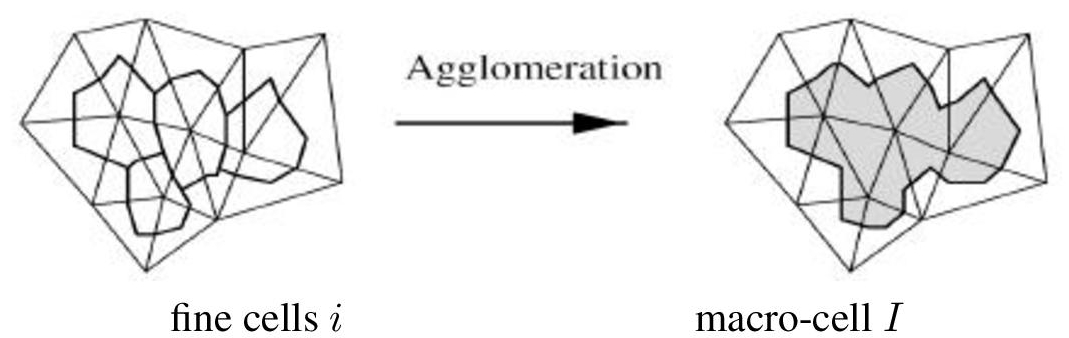
Figure 3.1. Sketch (in 2D) of the agglomeration of four cells into a macro-cell. Cells are dual cells of triangles, bounded by sections of triangle medians
3.2.3. MR time advancing
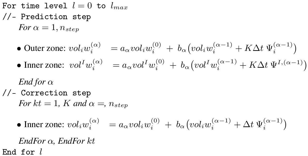
The MR algorithm is based on a prediction step and a correction step as defined hereafter:
Step 1 (prediction step):
The solution is advanced in time with time step KΔt; on the fine cells in the outer zone and on the macro-cells in the inner zone (which means using the macro-cell volumes and the coarse fluxes as defined in expression [3.1]):
For α = 1, nstep
EndFor α,
where wI,(α) denotes the fluid/turbulent variables at macro-cell I and stage α, (aα, bα) are the multi-stage parameters, a1 = 0, a2 = 3/4, a3 = 1/3 and b1 = 1, b2 = 1/4, b3 = 2/3 for the three-stage time advancing and volI is the volume of macro-cell I. From a practical point of view, we do not introduce in our software a new variable wI to that already existing wi. The previous sequence [3.3] is actually
On the other hand, the coarse fluxes ΨI are not stored in a specific variable, which means that no extra storage is necessary than the one required to store the fluxes Ψi1. Indeed, after the computation of the fluxes ![]() (using the values of
(using the values of ![]() ) at each stage α of the multi-stage time-advancing scheme, the coarse flux ΨI,(α−1) is evaluated according to expression [3.1] for each macro-cell I and then stored in the memory space allocated to
) at each stage α of the multi-stage time-advancing scheme, the coarse flux ΨI,(α−1) is evaluated according to expression [3.1] for each macro-cell I and then stored in the memory space allocated to ![]() for each cell i in the inner zone belonging to the macro-cell I.
for each cell i in the inner zone belonging to the macro-cell I.
Step 2 (correction step):
– The unknowns in the outer zone are frozen at level tn + KΔt.
– The unknowns in the outer zone close to the inner zone, which are necessary for advancing in time the inner zone (which means those which are useful for the computation of the fluxes Ψi in the inner zone), are interpolated in time.
– Using these interpolated values for the computation of the fluxes Ψi in the inner zone (at each stage of the time-advancing scheme), the solution in the inner zone is advanced K times in time with the chosen explicit scheme and time step Δt.
This time advancing is written as:
For kt = 1, K
For α = 1, nstep
EndFor α.
EndFor kt.
The arithmetic complexity is proportional to the number of points in the inner zone. The global multi-rate algorithm is presented in Algorithm 3.2.
Algorithm 3.2. Multi-rate time-advancing algorithm
3.3. Elements of analysis
3.3.1. Stability
The central question concerning the coarse grid is the stability resulting from its use in the computation. Considering [3.1], we expect that the viscous stability limit will improve by a factor four (1D) for a twice larger cell. The viscous stability limit can therefore be considered as more easily addressed by our coarsening. For the advective stability limit, we can be a little more precise. The coarse mesh is an unstructured partition of the domain in which cells are polyhedra. Analyses of time-advancing schemes on unstructured meshes are available in L2 norm for unstructured meshes (see Angrand and Dervieux 1984 and Giles 1997b, 1987). Here, we solely propose a L∞ analysis of the advection scheme. The gain in L∞ stability can be analyzed for a first-order upwind advection scheme. We get the following (obvious) lemma:
LEMMA 3.1.– The upwind advection scheme is positive on the mesh made of macro-cells as soon as for all macro-cell I:
where N (I) holds for the neighboring macro-cells of I. □
The application of an adequate neighboring-cell agglomeration, like in Lallemand et al. (1992) producing large macro-cells of good aspect ratio, will produce a K-times larger stability limit.
3.3.2. Accuracy
In contrast to more sophisticated MR algorithms, the proposed method has not a rigorous control of the accuracy. Let us however remark that the generic situation involves variable-size meshes, which limits the unsteady accuracy on small-scale propagation, already before applying the MR method. However, the two following remarks tend to show that the scheme accuracy is conserved:
– the predictor step involves simply a sum of the fluxes and the formal accuracy order is kept, with a coarser mesh size;
– still during the predictor step, if we assume that the mesh is reasonably smooth, then the CFL applied in the inner part near the matching zone will be close to the explicit CFL (applied on the outer part near the matching zone) and therefore accuracy is high.
Under these conditions, the effect of the corrector step will improve the result. In practice, most of our experiments will involve a comparison between the explicit time advancing and its MR extension.
3.3.3. Efficiency
The proposed two-level MR depends on only one parameter, the ratio K between the large and small time step. Considering a mesh with N vertices, a short loop on the mesh will produce the function ![]() which gives the number of cells in the inner region for K. If CPUExpNode(Δt) denotes the CPU per node and per time step Δt of the underlying explicit scheme, a model for the MR cpu per Δt would be
which gives the number of cells in the inner region for K. If CPUExpNode(Δt) denotes the CPU per node and per time step Δt of the underlying explicit scheme, a model for the MR cpu per Δt would be

to be compared with the explicit case
We shall call the expected gain the following ratio:
The above formula emphasizes the crucial influence on efficiency of a very small proportion of inner cells.
REMARK 3.1.– In most other multi-rate methods, the phase with a larger time-step does not concern the inner region and then their gain would be modeled by
Both gains are bounded by N/Nsmall(K) and show that this ratio has to be sufficiently large.
REMARK 3.2.– Once we have evaluated ![]() for a given mesh, it is possible to predict a theoretical optimum Kopt for minimizing the CPU time in scalar execution. However, we shall see that the pertinence of the above theory is lost by parallel implementation conditions.
for a given mesh, it is possible to predict a theoretical optimum Kopt for minimizing the CPU time in scalar execution. However, we shall see that the pertinence of the above theory is lost by parallel implementation conditions.
3.3.4. Toward many rates
Multi-rate strategies are supposed to extend to more than two different time step lengths while keeping a reasonable algebraic complexity. Let us examine the case of three lengths, namely Δt, KΔt, K2Δt. It is then necessary to generate two nested levels of agglomeration in such a way that Grid1 is stable for CFL =1, Grid2 is stable for CFL = K and Grid3 is stable for CFL = K2. While a two-rate calculation involves a prediction-correction based on Grid1 and Grid2,
– prediction on Grid2;
– correction on inner part of Grid1,
in a three-rate calculation, the correction step is replaced by two corrections:
– prediction on Grid3;
– correction on medium part of Grid2;
– correction on inner part of Grid1,
but this replacement is just the substitution (on a part of the mesh) of a single-rate advancing by a two-rate one and therefore can carry a higher efficiency (the smallest time step is restricted to a smaller inner zone). In contrast to other MR methods, we have a (second) duplication of flux assembly on the inner zone. However, this increment remains limited, since this computation is done 1 + K−1 + K−2 times (111% for K = 10).
3.3.5. Impact of our MR complexity on mesh adaption
We now check that the proposed MR indeed improves mesh adaption convergence order. Let us consider the space–time mesh used by a time-advancing method. A usual time advancing uses the Cartesian product {t0, t1, ...tN} × spatial mesh as space–time mesh. The space–time mesh is a measure of the computational cost since the discrete derivatives are evaluated on each node (tk, xk) of the Ntime × Nspace nodes of the space–time mesh. In Chapter 2 of Volume 1 and Chapters 2 and 7 of this volume, an analysis is proposed, which determines the maximal convergence order (in terms of number of space-time nodes) that can be attained on a given family of mesh. This analysis is useful for evaluating mesh-adaptive methods. For example, in Chapter 2 of Volume 1 and Chapter 7 of this volume, a 3D mesh-adaptive method for computing a traveling discontinuity has a convergence order α not better than αmax = 8/5, according to
d = 4 being the space–time dimension.
LEMMA 3.2.– Replacing the usual time-advancing by the MR algorithm will indeed improve the maximal convergence order of a mesh adaption method as defined in Chapters 2 and 7 of this volume.
PROOF.– Similarly to previous analyses, we restrict our argument to the case of the capture of a field involving a moving discontinuity. We have seen that anisotropic adaptation is able to generate a sequence of meshes for which eight times more vertices allows a four-times-smaller spatial error in the capture of the discontinuous function (spatial second-order). We have seen in Chapter 2 of Volume 1 that this property extends to transient fixed point mesh adaptation, giving again spatial second-order. We recall that, unfortunately, this needs to be combined with a four times smaller time step, so that in space-time, the number of degrees of freedom is multiplied by 8 × 4 = 32, which corresponds to a space-time convergence order limited to 8/5.
With an MR time advancing, the four times smaller time step can be restricted to the smallest spatial cells following the discontinuity. The number of points concerned is concentered along a 2D surface, so that their number can be evaluated by ![]() where Nspace is the total number of spatial vertices. On finer anisotropic mesh,
where Nspace is the total number of spatial vertices. On finer anisotropic mesh, ![]() is multiplied by 4 (2D division). Then when we divide space and time, and the amplification of CPU time can be evaluated as:
is multiplied by 4 (2D division). Then when we divide space and time, and the amplification of CPU time can be evaluated as:
that is with a factor:
for the proposed MR algorithm ![]() for a usual MR algorithm). Both formulas, for Nspace large, give the second order space-time convergence. □
for a usual MR algorithm). Both formulas, for Nspace large, give the second order space-time convergence. □
3.3.6. Parallelism
3.3.6.1. Implementation of MR
The proposed method needs be adapted to massive parallelism. We consider its adaptation to parallel MPI computation relying on mesh partitioning. In a preprocessing phase, the cell agglomeration is applied at run time inside each partition, which saves communications, and over the whole partition. The motivation is to do it once for the whole computation, while fluctuations of the inner zone at each time level will be taken into account by changing the list of active macro-cells to be agglomerated in the inner zone. Since our purpose is to remain with a rather simplified modification of the initial software, we did not modify the communication library (where we could to restrict the communications to the inner zone in the correction step).
To summarize, the MR algorithm involves at each time step:
– an updating of the inner zone (with a volume agglomeration done once for the computation);
– a prediction step that is similar to an explicit step (with a larger time step length), but with also a local sum of the fluxes in each macro-cell;
– a correction step that is similar to explicit arithmetics restricted to the inner region, and for simplicity of coding, communications that are left identical to the explicit advancing (communications applied to both inner and outer zones).
An intrinsic extra cost of our algorithm with respect to previous multi-rate algorithms is the computations on the inner zone during the predictor step. The correction step complexity is close to an explicit advancing one on the inner zone except the two phases of time interpolation and communications. Time interpolation can be implemented with a better efficiency by applying it only on a layer around the inner zone. However, the cost of the time interpolation is a very small part of the total cost. Global communications are less costly than 10% of the explicit time step cost. If the inner zone is 30% of the domain, developing communication restricted to inner zone will reduce the communication from 10% to 3% of the explicit time step on the whole domain, which shows that the correction step would be decreased from 40% to 33% of an explicit time stepping CPU.
3.3.6.2. Load balancing
The usual METIS software can be applied on the basis of a balanced partitioning of the mesh. However, as remarked in previous works (see, for example, Seny et al. 2014), if the mesh partition does not take into account the inner zone, then the work effort will not be balanced during the correction step. The bad work balance for the correction step can be of low impact if this step concerns a sufficiently small part of the mesh, resulting in a small part of the global work. However, a more reasonable assumption is that the correction phase represents a non-negligible part of the effort. In this section, we discuss the question of a partitioning taking into account the correction phase. We observe that in the proposed method the inner zone depends on the flow through the CFL condition. This means that dynamic load balancing may be useful in some case. It would be anyway compulsory if a strong mesh adaption like the algorithm described in Chapter 2 of this volume is combined with the multi-rate time advancing. However, in the class of flows which we consider, the change in inner zone can be neglected and we consider only static balancing. An option resulting from the work of Karypis and Kumar (2006) and available in METIS is the multi-constraint partitioning (MCP), which minimizes the communication cost with multiple constrains. The two constraints for MR are as follows:
– partition is balanced for the whole computational domain, which would be optimal for the prediction step;
– partition is balanced for the inner part of the computational domain, which would be optimal for the correction step.
More precisely, this partitioning algorithm produces a compromise among the following:
– making the number of nodes in each subdomain of the global mesh uniform;
– making the number of nodes in each subdomain of the inner part of the mesh uniform;
– minimizing the communications between the subdomains.
In some particular cases, the user can specify an evident partition that perfectly balances the number of nodes in each subdomain of the global mesh and in each subdomain of the inner part of the mesh. In our experiments, we explicitly specify when it is the case and how it is performed.
3.4. Applications
The MR algorithm is implemented into code Aironum. The spatial approximation is the superconvergent implementation of section 1.1.4 of Volume 1 of Chapter 1 and the circumcenter cells are used (Appendix of Chapter 1 of Volume 1). The superconvergent implementation of section 1.1.4 of Chapter 1 of Volume 1 is used. The explicit time advancing is a three-stage Shu method. The mean CPU for an explicit time step per mesh node varies between 10−7 and 4 × 10⁻⁷ s according to the partition quality and the number of nodes per subdomain.
3.4.1. Circular cylinder at very high Reynolds number
The discussion concerning the parallel processing of the multi-rate scheme will rely on a non-adaptative application. It is the simulation of the flow around a circular cylinder at Reynolds number 8.4 × 10⁶. A hybrid RANS/VMS-LES model is used to compute this flow. The complete model is described in Itam et al. (2018). Mean flow variables and turbulent variables are advanced by the time integration scheme, and therefore also the MR method. The computational domain is made up of small cells around the body in order to allow a proper representation of the very thin boundary layer that occurs at such a high Reynolds number. Figure 3.2 depicts the Q-criterion isosurfaces and shows the very small and complex structures that need to be captured by the numerical and the turbulence models, which renders this simulation very challenging.
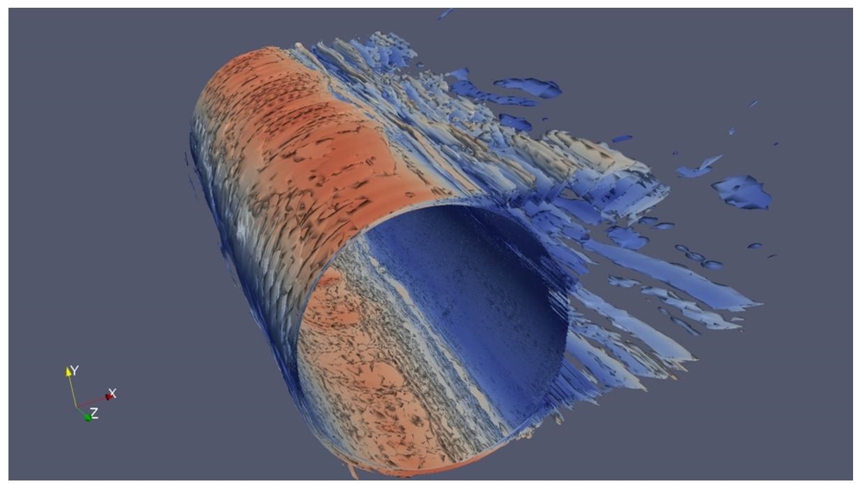
Figure 3.2. Circular cylinder at Reynolds number 8.4 × 10⁶. Instantaneous Q-criterion isosurfaces (colored with velocity modulus). For a color version of this figure, see www.iste.co.uk/dervieux/meshadaptation2
The mesh used in this simulation contains 4.3 million nodes and 25 million tetrahedra. The smallest cell thickness is 2.5 × 10⁻⁶. The computational domain is decomposed into 192 subdomains. When integer K, used for the definition of the inner and outer zones, is set to 5, 10 and 20, the percentage of nodes located in the inner zone is 15%, 19% and 24%, respectively (see Table 3.1).
Table 3.1. Circular cylinder at Reynolds number 8.4 × 10⁶. Time step factor K, number of processors, percentage of nodes in the inner region, theoretical gain in scalar mode, measured parallel gain, and relative error with respect to explicit time advancing, for MR (K = 2, 60) and implicit BDF2 (CFL = 30, 2). UP: usual partition; MCP: Metis multi-constrained partition; R: analytic radial optimal partition
| K | nproc | Expected gain (theoretical) | Measured gain (UP/MCP/R) | Error (%) | |
|---|---|---|---|---|---|
| 20 | 192 | 24 | 3.45 | 1.18/1.43/2.27 | 2.6 × 10⁻³ |
| 60 | 192 | 27 | 3.48 | 1.21/1.52/2.32 | 5 × 10⁻³ |
| BDF2 CFL=30 | 192 | 20./ − /− | 1.0 | ||
| CFL=2(est.) | 192 | 1.5/ − /− | 5 × 10⁻³ |
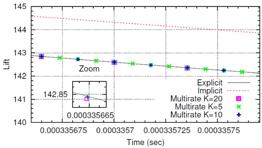
Figure 3.3. Circular cylinder at Reynolds number 8.4 × 10⁶. Zoom of the lift curves obtained with explicit, implicit and MR schemes. For a color version of this figure, see www.iste.co.uk/dervieux/meshadaptation2
For each simulation, 192 cores were used on a Bullx B720 cluster, and the CFL number was set to 0.5. CPU times for the explicit and MR schemes with different values of K are given in Table 3.1. One can observe that the efficiency of the MR approach is rather moderate, with however a noticeable improvement of the gain in the case of a radial optimal partition. The cost of the correction step is indeed relatively high compared to the prediction step. This is certainly due to an important number of inner nodes (which implies also a moderate theoretical scalar gain) and a non-uniform distribution of these nodes among the computational cores for the usual partition.
It is interesting to compare these performances with the efficiency of an implicit algorithm. The implicit algorithm (BDF2) that we use is advanced with a GMRES linear solver using a Restrictive-Additive Schwarz preconditioner and ILU(0) in each partition (see Koobus et al. 2011 for further details). In the cases computed with the implicit scheme, the CFL is fixed to 30 and the total number of GMRES iterations for one time step is around 20. For this CFL, the gain of an implicit computation with respect to an explicit one at CFL 0.5 is measured between 12 and 22 depending on the number of nodes per processor. The BDF2 algorithm is second-order accurate in time and we shall use this property when estimating which time step reduction is necessary for reducing by a given factor the deviation with respect to explicit time advancing. An important gain is observed as compared to the MR case, but at the cost of a degradation of the accuracy (see Table 3.1 and Figure 3.3). This is probably related to the small-scale fluctuations, which arise at this Reynolds number (Figure 3.2). They need to be captured with a rather accurate time advancing. A 1% deviation after a shedding cycle may become 20% after 20 cycles and deteriorate the prediction of bulk fluctuations. In order to obtain the same level of error, the implicit time advancing, which is second-order accurate in time, should be run with a CFL of 2, with a gain of only 1.5 (less than the MR case with the radial optimal partition).
3.4.2. Mesh adaption for a contact discontinuity
This example is a simplified case of mesh adaptation. We consider the case of a moving contact discontinuity. For this purpose, the compressible Euler equations are solved in a rectangular parallelepiped as computational domain where the density is initially discontinuous at its middle (see Figure 3.4) while velocity and pressure are uniform.

Figure 3.4. Mesh adaptative calculation of a traveling contact discontinuity. Instantaneous mesh with mesh concentration in the middle of zoom and corresponding advected discontinuous fluid density. Density is 3 on the left, 1 on the right. For a color version of this figure, see www.iste.co.uk/dervieux/meshadaptation2
The uniform velocity is a purely horizontal one. As can be seen in Figure 3.4, small cells are present on either side of the discontinuity. The mesh adapts analytically during the computation in such a way that the nodes located at the discontinuity are still the same, and the number of small cells are equally balanced on either side of the discontinuity. An Arbitrary Lagrangian-Eulerian formulation is then used to solve the Euler equations on the resulting deforming mesh. Our long term objective is to combine the MR time advancing with a mesh adaptation algorithm in such a way that the small time steps imposed by the necessary good resolution of the discontinuity remain of weak impact on the global computational time. The 3D mesh used in this simulation contains 25,000 vertices. The computational domain is divided into two subdomains, the partition interface being defined in such a way that it follows the center plan of the discontinuity. When integer K, used for the definition of the inner and outer zones, is set to 5, 10 and 15, the percentage of nodes located in the inner zone is always 1.3%, which corresponds to the vertices of the small cells located on either side of the discontinuity. The CFL with respect to propagation is 0.5. The MR scheme with the aforementioned values of K is used for the computation. Each simulation is run on 2 cores of a Bullx B720 cluster. In Table 3.2, CPU times (prediction step/correction step) are given for the MR approach and different time step factors K. The correction step, consists of explicit time advancing on inner zone, 1.3% of the mesh (solely 78 vertices on each partition), but, due to parallel and vector inefficiency, one Shu step of it is 39% of one Shu explicit step on the whole mesh.
Table 3.2. Mesh adaptative propagation of a contact discontinuity: Time step factor K, CPU of the explicit scheme per explicit time-step Δt and per node, percentage of nodes in the inner region, theoretical gain in scalar mode, CPU of the prediction step per time-step KΔt, CPU of the correction step per time-step KΔt and measured parallel gain
| K | Nsmall(K)/N (%) | Expected gain (theoretical) | CPU pred. step (s/KΔt) | CPU correc. step (s/KΔt) | Measured gain (parallel) |
|---|---|---|---|---|---|
| 5 | 1.3 | 4.7 | 0.124 | 0.244 | 1.7 |
| 10 | 1.3 | 8.8 | 0.124 | 0.482 | 2.0 |
| 15 | 1.3 | 12.5 | 0.124 | 0.729 | 2.2 |
3.5. Conclusion
The motivation for using a multi-rate approach is twofold. First, with the arising of novel anisotropic mesh adaptation methods, the complexity of unsteady accurate computations with large and small mesh sizes needs to be reduced. Second, we are interested by increasing the efficiency of accurate unsteady simulations. Of course, the very high Reynolds number hybrid simulations can be computed with implicit time advancing for maintaining a reasonable cpu. But in many cases this is done with an important degradation of the accuracy with respect to smaller time steps on the same mesh.
The proposed method is based on control volume agglomeration, and relies on:
– a prediction step where large time steps are used and where the fluxes for the smaller elements are evaluated on macro-cells for stability purpose;
– a correction step in which only the smaller elements of the so-called inner zone are advanced in time with a small time step.
An important interest of the method is that the modification effort in an existing explicit unstructured code is very low. Results show that the proposed MR strategy can be applied to complex unsteady CFD problems such as the prediction of three-dimensional flows around bluff bodies with a hybrid RANS/LES turbulence model. A simplified mesh adaptive calculation of a moving shock is also performed, as a preliminary test for mesh adaptation. All the numerical experiments are in parallel computed with MPI. This allows to identify the main difficulty in obtaining high computational gain, which is related with the parallel efficiency of the computations restricted to the inner zone. Because of the use of an explicit Runge–Kutta time advancing, the time accuracy of the MR scheme remains high and the dissipation remains low, as compared with an implicit computation. Only very small time scales are lost with respect to a pure explicit computation. Implicit accuracy is limited not only by the intrinsic scheme accuracy but also by the conditions required to achieve greater efficiency, which involve a sufficiently large time step and a short, parameter dependant, convergence of the linear solver performed in the time-advancing step. In contrast, explicit and MR computations are parameter safe, and the accuracy of the MR method is optimal in regions complementary to the inner zone.
3.6. Notes
Most contents of this chapter are borrowed from (Itam et al. 2019), which present some other numerical experiments.
About multi-rate works. The multi-rate methods starts from Skelboes’s pioneering work using backward differentiation formulas (BDF) (Skelboe 1989) and continues to recent works dealing with hyperbolic conservation laws (Constantinescu and Sandu 2007; Sandu and Constantinescu 2009; Mugg 2012; Seny et al. 2014).
For the solution of ODEs or EDPs, explicit integration schemes are still often used because of the accuracy they can provide and their simplicity of implementation. Nevertheless, these schemes can prove to be very expensive in some situations, for example, stiff ODEs whose solution components exhibit different time scales, system of non-stiff ODEs characterized by different activity levels (fast/slow), or EDPs discretized on computational grids with very small elements. In order to overcome this efficiency problem, different strategies were developed, first in the field of ODEs, in order to propose an interesting alternative:
– multi-method schemes: for systems of ODEs containing both non-stiff and stiff parts, an explicit scheme is used for the non-stiff subsystem and an implicit method for the stiff one (Hofer 1976; Rentrop 1985; Weiner et al. 1993);
– multi-order schemes: for non-stiff system of ODEs, the same explicit method and step size are used, but the order of the method is selected according to the activity level (fast/slow) of the considered subsystem of ODEs (Engstler and Lubich 1997a);
– multi-rate schemes: for stiff and non-stiff problems, the same explicit or implicit method with the same order is applied to all subsystems, but the step size is chosen according to the activity level. The first multi-rate time integration algorithm goes back to the work of Rice (1960).
In what follows, we focus our review on the multi-rate approach. The application of such schemes was first limited to ODEs (Rice 1960; Andrus 1979; Gear 1971; Skelboe 1989; Sand and Skelboe 1992; Andrus 1993; Günther and Rentrop 1993; Engstler and Lubich 1997b,a; Günther et al. 1998, 2001; Savcenco et al. 2007) and restricted to a low number of industrial problems. In the past 15 years, the development and application of such methods to the time integration of PDEs was also performed. In particular, a few works were conducted on the system of ODEs that arise after semidiscretization of hyperbolic conservation laws (Constantinescu and Sandu 2007; Sandu and Constantinescu 2009; Mugg 2012; Kirby 2002; Seny et al. 2014; Löhner et al. 1984), and rare applications were performed in computational fluid dynamics (CFD) (Seny et al. 2014; Löhner et al. 1984) for which we are interested.
The work of Skelboe on multi-rate BDF methods, 1989 (Skelboe 1989). In this work, concerning multi-rate BDF schemes, first-order ODEs, made of a fast subsystem and a slow subsystem, are considered. In the proposed multi-rate strategy, the fast subsystem is integrated by a k-step BDF formula (BDF-k) with step length h, and the slow subsystem is integrated by the same BDF-k formula but with time step H = qh, where q is an integer multiplying factor. Interpolation and extrapolation values (following a Newton type formula) of the solution are used in the proposed algorithms.
As for the application part, a 2 × 2 test problem is considered for investigating the stability properties of the multi-rate algorithms. From this application, it appears that the proposed multi-rate algorithms are not necessarily A-stable, limiting the use of such methods.
The work of Günther and Rentrop on multi-rate Rosenbrock-Wanner (ROW) methods, 1993 (Günther and Rentrop 1993). In this work, regarding multi-rate ROW algorithms, autonomous first-order ODEs, which can be split into active and latent components, are considered. The multi-rate strategy is based on a ROW method in which a large time step H is used for the latent subsystem and a small time step h = H/m is employed for advancing the active components of the solution. In the proposed multi-rate method, the latent and active components of the solution are extrapolated using a Padé approximation.
The application part concerns the simulation of electric circuits (inverter chain) leading to the solution of stiff ODEs (system of 250–4000 differential equations). A multi-rate four-step ROW method was implemented, leading to a A-stable algorithm, and a speedup up to 2.8 compared to the classical explicit four-stage Runge Kutta (RK) method.
The work of Löhner-Morgan-Zienkiewicz on explicit multi-rate schemes for hyperbolic problems with CFD applications, 1984 (Löhner et al. 1984). To our knowledge, this work is the first one on multi-rate methods that deals with applications in CFD. In the model problem, two subregions with different grid resolution are considered and the solution is advanced in time using a given explicit scheme. A large time step Δt1 is used in the coarse subregion Ω1, and a small time step Δt2 =Δt1/n is employed in the fine subregion Ω2. In the proposed multi-rate strategy, some grid points belonging to Ω1 are added to the fine subregion Ω2 (which becomes ![]() ), and appropriate boundary conditions are used for both subregions Ω1 and
), and appropriate boundary conditions are used for both subregions Ω1 and ![]() together with mean values at some points belonging to Ω1 and
together with mean values at some points belonging to Ω1 and ![]() The proposed multi-rate scheme was implemented with a second-order explicit finite element scheme (Taylor-Galerkin method of Donea).
The proposed multi-rate scheme was implemented with a second-order explicit finite element scheme (Taylor-Galerkin method of Donea).
Several CFD test cases were considered, which illustrate that shocks can be handled by the multi-rate method and that a speedup of 2 between the multi-rate scheme and its single-rate counterpart can be obtained.
The work of Kirby on a multi-rate forward Euler scheme for hyperbolic conservation laws, 2002 (Kirby 2002). This theoretical work presents and analyzes a multi-rate method for the solution of one-dimensional hyberbolic conservation laws. After semi-discretization by a finite volume MUSCL approach, a system of ODEs is obtained which is partitioned in fast and slow subsystems. A rather simple multi-rate scheme based on forward Euler steps is proposed for the solution of these subsystems. The fast subsystem is advanced with a small time step Δt/m, while a large time step Δt is used for the slow subsystem. No extrapolation/interpolation are performed in the proposed multi-rate strategy. It is shown that the multi-rate scheme satisfies the TVD property and a maximum principle under local CFL conditions, but it is only first order time accurate.
The work of Constantinescu and Sandu on multi-rate RK methods for hyperbolic conservation laws, 2007 (Constantinescu and Sandu 2007). One-dimensional scalar hyperbolic equations are considered in this study. For the solution of these equations, a second-order accurate multi-rate scheme that inherits stability properties of the single rate integrator (maximum principle, TVD, TVB, monotocity-preservation, positivity) is developed. After a semi-discrete finite volume approximation (which satisfies some of the above stability properties), a system of ODEs is obtained and divided into slow and fast subsystems. The computational domain is split into a subdomain ΩF corresponding to a fast characteristic time where a small time step Δt/m is used in the multi-rate scheme and a subdomain ΩS with a slow characteristic time where a large time step Δt is employed. Furthermore, a buffer zone between ΩF and ΩS is introduced in order to bridge the transition between these two subdomains for the purpose that the multi-rate scheme satisfies the stability properties of the single rate scheme. In the proposed multi-rate method, appropriate explicit RK schemes are also used in each subdomain and the buffer zone.
The resulting multi-rate algorithm is assessed on 1D problems (advection equation, and Burger’s equation) with fixed and moving grids. It was checked that the numerical solutions are second-order accurate, positive, obey the maximum principle, TVD, wiggle free, and the integration is conservative. Speedups up to 2.4 were obtained.
The work of Seny et al. on the parallel implementation of multi-rate RK methods, 2014 (Seny et al. 2014). This work focuses on the efficient parallel implementation of explicit multi-rate RK schemes in the framework of discontinuous Galerkin methods. The multi-rate RK scheme used is the approach proposed by Constantinescu and Sandu (2007) and introduced in the previous section.
In order to optimize the parallel efficiency of the multi-rate scheme, they propose a solution based on multi-constraint mesh partitioning. The objective is to ensure that the workload, for each stage of the multi-rate algorithm, is almost equally shared by each computer core, that is, the same number of elements are active on each core, while minimizing inter-processor communications. The METIS software is used for the mesh decomposition, and the parallel programing is performed with the message passing interface.
The efficiency of the parallel multi-rate strategy is evaluated on two- and three-dimensional CFD problems. It is shown that the multi-constraint partitioning strategy increases the efficiency of the parallel multi-rate scheme compared to the classical single-constraint partitioning. However, they observe that strong scalability is achieved with more difficulty with the multi-rate algorithm than with its single rate counterpart, especially when the number of processors becomes important compared to the number of mesh elements. The possible low number of elements per multi-rate group and per processor is a limiting factor for the proposed approach.
Notes
- 1 A more efficient implementation would not compute the fluxes between two internal cells of a macro-cell.