
2
Schema Design and Data Modeling
This chapter will focus on schema design for schemaless databases such as MongoDB. Although this may sound counterintuitive, there are considerations that we should take into account when we develop for MongoDB. We will learn about the schema considerations and the data types supported by MongoDB. We will also learn about preparing data for text searches in MongoDB by connecting using Ruby, Python, and PHP.
By the end of this chapter, you will have learned how to connect to MongoDB using the Ruby, Python, and PHP languages and using the low-level driver commands or an object-relational mapping framework. You will have learned how to model your data for different entity relationship mappings and what the trade-offs of different design decisions are.
In this chapter, we will cover the following topics:
- Relational schema design
- Data modeling
- Modeling data for atomic operations
- Modeling relationships
- Connecting to MongoDB
Technical requirements
To follow along with the code in this chapter, you need to install MongoDB locally or connect to a MongoDB Atlas database using a UNIX type system. You can download the MongoDB Community Edition from mongodb.com or use the fully managed DBaaS MongoDB Atlas offering, which provides a free tier as well as seamless upgrades to the latest version.
You will also need to download the official drivers for the language of your choice – Ruby, Python, or PHP. Finally, you will need to download MongoId, PyMODM, or Doctrine ODM frameworks for the respective languages. You can find all the code from this chapter in the GitHub repository at https://github.com/PacktPublishing/Mastering-MongoDB-6.x.
Relational schema design
In relational databases, we design with the goal of avoiding data anomalies and data redundancy.
Data anomalies can happen when we have the same information stored in multiple columns; we update one of them but not the rest and so end up with conflicting information for the same column of information.
Another example of a data anomaly is when we cannot delete a row without losing the information that we need, possibly in other rows referenced by it.
Data redundancy on the other hand refers to a situation where our data is not in a normal form but has duplicate data across different tables. This can lead to data inconsistency and make the data integrity difficult to maintain.
In relational databases, we use normal forms to normalize our data. Starting from the basic first normal form (1NF), onto the second normal form (2NF), third normal form (3NF), and Boyce-Codd normal form (BCNF), there are different ways to model our data. We structure our tables and columns by using functional dependencies between different data units. Following this formal method, we can prove that our data is normalized, with the downside that we can sometimes end up with many more tables than the domain model objects that we originally started with from our systems model.
In practice, relational database modeling is often driven by the structure of the data that we have. In web applications following some sort of model-view-controller (MVC) model pattern, we will model our database according to our models that are based on the Unified Modeling Language (UML) diagram conventions. Abstractions such as the ORM for Django or the Active Record for Rails help application developers abstract database structure to object models. Ultimately, many times, we end up designing our database based on the structure of the available data. Therefore, we are designing around the questions that we need to answer.
MongoDB schema design
In contrast to relational databases, in MongoDB, we have to base our modeling on our application-specific data access patterns. Finding out the questions that our users will have is paramount to designing our entities. In contrast to an RDBMS, data duplication and denormalization are used far more frequently, for good reason.
The document model that MongoDB uses means that every document can hold substantially more or less information than the next one, even within the same collection. Coupled with rich and detailed queries being possible in MongoDB at the embedded document level, this means that we are free to design our documents in any way that we want. When we know our data access patterns, we can estimate which fields need to be embedded and which can be split out into different collections.
Read-write ratio
The read-write ratio is often an important design consideration for MongoDB modeling. When reading data, we want to avoid scatter-gather situations, where we have to hit several shards with random I/O requests to get the data that our application needs.
When writing data, on the other hand, we want to spread out writes to as many servers as possible to avoid overloading any single one of them. These goals appear to be conflicting on the surface, but they can be combined once we know our access patterns, coupled with application design considerations, such as using a replica set to read from secondary nodes.
Data modeling
In this section, we will discuss the different types of data MongoDB uses, how they map to the data types that programming languages use, and how we can model data relationships in MongoDB using Ruby, Python, and PHP.
Data types
MongoDB uses BSON, a binary-encoded serialization for JSON documents. BSON extends the JSON data types, offering, for example, native data and binary data types.
BSON, compared to protocol buffers, allows for more flexible schemas, which comes at the cost of space efficiency. In general, BSON is space-efficient, easy to traverse, and time-efficient in encoding/decoding operations, as can be seen in the following table (see the MongoDB documentation at https://docs.mongodb.com/manual/reference/bson-types/):

Table 2.1 – MongoDB data types
In MongoDB, we can have documents with different value types for a given field and we can distinguish between them when querying using the $type operator.
For example, if we have a balance field in GBP with 32-bit integers and double data types, and based on whether the balance field has in it or not, we can easily query by $type for all accounts that have a rounded balance field, with any of the following queries shown in the example:
db.account.find( { "balance" : { $type : 16 } } );db.account.find( { "balance" : { $type : "integer" } } );We will compare the different data types in the following section.
Comparing different data types
Due to the nature of MongoDB, it’s perfectly acceptable to have different data type objects in the same field. This may happen by accident or on purpose (that is, null and actual values in a field).
The sorting order of different types of data, from highest to lowest, is as follows:
- Max. key (internal type)
- Regular expression
- Timestamp
- Date
- Boolean
- ObjectID
- Binary data
- Array
- Object
- Symbol, string
- Numbers (int, long, double, Decimal128)
- Null
- Min. key (internal type)
Non-existent fields get sorted as if they have null in the respective field. Comparing arrays is a bit more complex than fields. Ascending order of comparison (or <) will compare the smallest element of each array. Descending order of comparison (or >) will compare the largest element of each array.
For example, see the following scenario:
> db.types.find()
{ "_id" : ObjectId("5908d58455454e2de6519c49"), "a" : [ 1, 2, 3 ] }
{ "_id" : ObjectId("5908d59d55454e2de6519c4a"), "a" : [ 2, 5 ] }
In ascending order, this is as follows:
> db.types.find().sort({a:1})
{ "_id" : ObjectId("5908d58455454e2de6519c49"), "a" : [ 1, 2, 3 ] }
{ "_id" : ObjectId("5908d59d55454e2de6519c4a"), "a" : [ 2, 5 ] }
However, in descending order, it is as follows:
> db.types.find().sort({a:-1})
{ "_id" : ObjectId("5908d59d55454e2de6519c4a"), "a" : [ 2, 5 ] }
{ "_id" : ObjectId("5908d58455454e2de6519c49"), "a" : [ 1, 2, 3 ] }
The same applies when comparing an array with a single number value, as illustrated in the following example. Inserting a new document with an integer value of 4 is done as follows:
> db.types.insert({"a":4})
WriteResult({ "nInserted" : 1 })
The following example shows the code snippet for a descending sort:
> db.types.find().sort({a:-1})
{ "_id" : ObjectId("5908d59d55454e2de6519c4a"), "a" : [ 2, 5 ] }
{ "_id" : ObjectId("5908d73c55454e2de6519c4c"), "a" : 4 }
{ "_id" : ObjectId("5908d58455454e2de6519c49"), "a" : [ 1, 2, 3 ] }
And the following example is the code snippet for an ascending sort:
> db.types.find().sort({a:1})
{ "_id" : ObjectId("5908d58455454e2de6519c49"), "a" : [ 1, 2, 3 ] }
{ "_id" : ObjectId("5908d59d55454e2de6519c4a"), "a" : [ 2, 5 ] }
{ "_id" : ObjectId("5908d73c55454e2de6519c4c"), "a" : 4 }
In each case, we have highlighted the values being compared in bold.
We will learn about the date type in the following section.
Date types
Dates are stored as milliseconds, with effect from January 01, 1970 (epoch time). They are 64-bit signed integers, allowing for a range of 135 million years before and after 1970. A negative date value denotes a date before January 01, 1970. The BSON specification refers to the date type as UTC DateTime.
Dates in MongoDB are stored in UTC. There isn’t a timestamp field with a timezone data type like in some relational databases. Applications that need to access and modify timestamps based on local time should store the timezone offset together with the date and offset dates on an application level.
In the MongoDB shell, this could be done using the following format with JavaScript:
var now = new Date();
db.page_views.save({date: now,offset: now.getTimezoneOffset()});
Then, you need to apply the saved offset to reconstruct the original local time, as in the following example:
var record = db.page_views.findOne();
var localNow = new Date( record.date.getTime() - ( record.offset * 60000 ) );
In the next section, we will cover ObjectId.
ObjectId
ObjectId is a special data type for MongoDB. Every document has an _id field from cradle to grave. It is the primary key for each document in a collection and has to be unique. If we omit this field in a create statement, it will be assigned automatically with an ObjectId data type.
Messing with ObjectId is not advisable but we can use it (with caution!) for our purposes.
ObjectId has the following distinctions:
- It has 12 bytes
- It is ordered
- Sorting by _id will sort by creation time for each document, down to one-second granularity
- The creation time can be accessed by .getTimeStamp() in the shell
The structure of an ObjectId value consists of the following:
- The first four bytes are the seconds since the Unix epoch, 00:00:00 UTC on January 01, 1970.
- The next five bytes are unique to the device and process. They are generated randomly with the first three bytes being the machine identifier and the next two the process ID.
- The last three bytes represent an incrementing counter, starting with a random value.
The following diagram shows the structure of an ObjectId value:

Figure 2.1 – Internal structure of the ObjectId value
By design, ObjectId will be unique across different documents in replica sets and sharded collections.
In the next section, we will learn about modeling data for atomic operations.
Modeling data for atomic operations
MongoDB is relaxing many of the typical Atomicity, Consistency, Isolation, and Durability (ACID) constraints found in RDBMS. The default operation mode does not support transactions, making it important to keep the state consistent across operations, especially in the event of failures.
Some operations are atomic at the document operation level:
- update()
- findandmodify()
- remove()
These are all atomic (all-or-nothing) for a single document.
This means that, if we embed information in the same document, we can make sure they are always in sync.
An example would be an inventory application, with a document per item in our inventory. Every time a product is placed in a user’s shopping cart, we decrement the available_now value by one and append the userid value to the shopping_cart_by array.
With total_available = 5, available_now = 3, and shopping_cart_count = 2, this use case could look like the following:
{available_now : 3, shopping_cart_by: ["userA", "userB"] }When someone places the item in their shopping cart, we can issue an atomic update, adding their user ID in the shopping_cart_by field and, at the same time, decreasing the available_now field by one.
This operation will be guaranteed to be atomic at the document level. If we need to update multiple documents within the same collection, the update operation may complete successfully without modifying all of the documents that we intended it to. This could happen because the operation is not guaranteed to be atomic across multiple document updates.
This pattern can help in some but not all cases. In many cases, we need multiple updates to be applied on all or nothing across documents, or even collections.
A typical example would be a bank transfer between two accounts. We want to subtract x GBP from user A, then add x to user B. If we fail to do either of these two steps, both balances would return to their original state.
Since version 4, we should use multi-document transactions in such cases, which we will cover in Chapter 6, Multi-Document ACID Transactions.
In the next section, we will learn more about the visibility of MongoDB operations between multiple readers and writers.
Read isolation and consistency
MongoDB read operations would be characterized as read uncommitted in a traditional RDBMS definition. What this means is that, by default, reads can get values that may not finally persist to the disk in the event of, for example, data loss or a replica set rollback operation.
In particular, when updating multiple documents with the default write behavior, lack of isolation may result in the following:
- Reads may miss documents that were updated during the update operations
- Non-serializable operations
- Read operations are not point-in-time
Queries with cursors that don’t use .snapshot() may also, in some cases, get inconsistent results. This can happen if the query’s resultant cursor fetches a document that receives an update while the query is still fetching results, and, because of insufficient padding, ends up in a different physical location on the disk, ahead of the query’s result cursor position. .snapshot() is a solution for this edge case, with the following limitations:
- It doesn’t work with sharding
- It doesn’t work with sort() or hint() to force an index to be used
- It still won’t provide point-in-time read behavior
If our collection has mostly static data, we can use a unique index in the query field to simulate snapshot() and still be able to apply sort() to it.
All in all, we need to apply safeguards at the application level to make sure that we won’t end up with unexpected results.
Starting from version 3.4, MongoDB offers linearizable read concern. With linearizable read concern from the primary member of a replica set and a majority write concern, we can ensure that multiple threads can read and write a single document as if a single thread were performing these operations one after the other. This is considered a linearizable schedule in RDBMS, and MongoDB calls it the real-time order.
Starting from version 4.4, we can set a global default read concern on the replica set and sharded cluster level. The implicit write concern is w:majority, which means that the write will be acknowledged after it’s been propagated to a majority of the nodes in the cluster.
If we use a read concern that is majority or higher, then we can make sure that the data we read is write-committed in the majority of nodes, making sure that we avoid the read uncommitted problem that we described at the beginning of this section.
Modeling relationships
In the following sections, we will explain how we can translate relationships in RDBMS theory into MongoDB’s document collection hierarchy. We will also examine how we can model our data for text search in MongoDB.
One-to-one
Coming from the relational DB world, we identify objects by their relationships. A one-to-one relationship could be a person with an address. Modeling it in a relational database would most probably require two tables: a person and an address table with a person_id foreign key in the address table, as shown in the following diagram:

Figure 2.2 – Foreign key used to model a one-to-one relationship in MongoDB
The perfect analogy in MongoDB would be two collections, Person and Address, as shown in the following code:
> db.Person.findOne()
{
"_id" : ObjectId("590a530e3e37d79acac26a41"), "name" : "alex"
}
> db.Address.findOne()
{
"_id" : ObjectId("590a537f3e37d79acac26a42"),
"person_id" : ObjectId("590a530e3e37d79acac26a41"),
"address" : "N29DD"
}
Now, we can use the same pattern as we do in a relational database to find Person from address, as shown in the following example:
> db.Person.find({"_id": db.Address.findOne({"address":"N29DD"}).person_id})
{
"_id" : ObjectId("590a530e3e37d79acac26a41"), "name" : "alex"
}
This pattern is well known and works well in the relational world.
Note
The command is performing two queries nested inside one another, the first one to retrieve the person_id _id value, which we use to query the Person collection by _id.
In MongoDB, we don’t have to follow this pattern, as there are more suitable ways to model this kind of relationship.
One way in which we would typically model one-to-one or one-to-many relationships in MongoDB would be through embedding. If the person has two addresses, then the same example would then be shown in the following way:
{ "_id" : ObjectId("590a55863e37d79acac26a43"), "name" : "alex", "address" : [ "N29DD", "SW1E5ND" ] }
Using an embedded array, we can access every address that this user has. Embedding querying is rich and flexible so that we can store more information in each document, as shown in the following example:
{ "_id" : ObjectId("590a56743e37d79acac26a44"),
"name" : "alex",
"address" : [ { "description" : "home", "postcode" : "N29DD" },
{ "description" : "work", "postcode" : "SW1E5ND" } ] }
The advantages of this approach are as follows:
- No need for two queries across different collections
- It can exploit atomic updates to make sure that updates in the document will be all-or-nothing from the perspective of other readers of this document
- It can embed attributes in multiple nest levels, creating complex structures
The most notable disadvantage is that the maximum size of the document is 16 MB, so this approach cannot be used for an arbitrary, ever-growing number of attributes. Storing hundreds of elements in embedded arrays will also degrade performance.
One-to-many and many-to-many
When the number of elements on the many side of the relationship can grow unbounded, it’s better to use references. References can come in two forms:
- From the one side of the relationship, store an array of many-sided elements, as shown in the following example:
> db.Person.findOne()
{ "_id" : ObjectId("590a530e3e37d79acac26a41"), "name" : "alex", addresses:
[ ObjectID('590a56743e37d79acac26a44'),
ObjectID('590a56743e37d79acac26a46'),
ObjectID('590a56743e37d79acac26a54') ] }
- This way, we can get the array of the addresses elements from the one side and then query with in to get all the documents from the many side, as shown in the following example:
> person = db.Person.findOne({"name":"mary"})
> addresses = db.Addresses.find({_id: {$in: person.addresses} })
Turning this one-to-many into many-to-many is as easy as storing this array at both ends of the relationship (that is, in the Person and Address collections).
- From the many side of the relationship, store a reference to the one side, as shown in the following example:
> db.Address.find()
{ "_id" : ObjectId("590a55863e37d79acac26a44"), "person": ObjectId("590a530e3e37d79acac26a41"), "address" : [ "N29DD" ] }
{ "_id" : ObjectId("590a55863e37d79acac26a46"), "person": ObjectId("590a530e3e37d79acac26a41"), "address" : [ "SW1E5ND" ] }
{ "_id" : ObjectId("590a55863e37d79acac26a54"), "person": ObjectId("590a530e3e37d79acac26a41"), "address" : [ "N225QG" ] }
> person = db.Person.findOne({"name":"alex"})
> addresses = db.Addresses.find({"person": person._id})
As we can see, with both designs we need to make two queries to the database to fetch the information. The second approach has the advantage that it won’t let any document grow unbounded, so it can be used in cases where one-to-many is one-to-millions.
Modeling data for keyword searches
Searching for keywords in a document is a common operation for many applications. We can search using an exact match or by using a $regex regular expression in the content of a field that contains text. MongoDB also provides the ability to search using an array of keywords.
The basic need for a keyword search is to be able to search the entire document for keywords. For example, there could be a need to search a document in the products collection, as shown in the following code:
{ name : "Macbook Pro late 2016 15in" ,manufacturer : "Apple" ,
price: 2000 ,
keywords : [ "Macbook Pro late 2016 15in", "2000", "Apple", "macbook", "laptop", "computer" ]
}
We can create a multikey index in the keywords field, as shown in the following code:
> db.products.createIndex( { keywords: 1 } )Now, we can search in the keywords field for any name, manufacturer, price, and also any of the custom keywords that we set up. This is not an efficient or flexible approach, as we need to keep keywords lists in sync, we can’t use stemming, and we can’t rank results (it’s more like filtering than searching). The only advantage of this method is that it is slightly quicker to implement.
A better way to solve this problem is by using the special text index type, now in version 3.
Only one text index per collection (except for Atlas Search SaaS) can be declared in one or multiple fields. The text index supports stemming, tokenization, exact phrase (“ “), negation (-), and weighting results.
Index declaration on three fields with custom weights is shown in the following example:
db.products.createIndex({name: "text",
manufacturer: "text",
price: "text"
},
{ weights: { name: 10,manufacturer: 5,
price: 1 },
name: "ProductIndex"
})
In this example, name is 10 times more important than price but only two times more important than manufacturer.
A text index can also be declared with a wildcard, matching all the fields that match the pattern, as shown in the following example:
db.collection.createIndex( { "$**": "text" } )This can be useful when we have unstructured data and we may not know all the fields that it will come with. We can drop the index by name, just like with any other index.
The greatest advantage though, other than all these features, is that all record keeping is done by the database.
Modeling data for Internet of Things
Internet of things (IoT) is one of the most quickly growing industries and this comes with unique challenges around data storage and processing. IoT systems typically use multiple sensors to gather data that needs to be stored, analyzed, and processed in near real time.
MongoDB introduced time series collections in version 5.0 and greatly extended supported functionality in version 6. These are special collections that are faster for data series that can contain sensor measurements.
For example, to create a time series collection, stocks with a timeField field of “timestamp”, and using the default granularity of “seconds” (or “minutes”, “hours”, et cetera) would require the following mongo shell command:
db.createCollection(
"stocks",
{
timeseries: {
timeField: "timestamp",
metaField: "metadata",
granularity: "seconds",
},
expireAfterSeconds: 3600,
}
)
metaField is a field that can store any kind of metadata that is useful for our querying, such as sensor-unique IDs.
expireAfterSeconds is optional and we can set it to allow MongoDB to auto-delete collection data after the threshold.
The time series collection has an index on timeField, so we can query it really effectively within any time period that we need. For more complex queries, we can use the aggregation framework.
In the next section, we will learn how to connect to MongoDB.
Connecting to MongoDB
There are two ways to connect to MongoDB. The first is by using the driver for your programming language. The second is by using an ODM layer to map your model objects to MongoDB in a transparent way. In this section, we will cover both ways, using three of the most popular languages for web application development: Ruby, Python, and PHP.
Connecting using Ruby
Ruby was one of the first languages to have support from MongoDB with an official driver. The official MongoDB Ruby driver on GitHub is the recommended way to connect to a MongoDB instance. Perform the following steps to connect MongoDB using Ruby:
- Installation is as simple as adding it to the Gemfile, as shown in the following example:
gem 'mongo', '~> 2.17'
- Then, in our class, we can connect to a database, as shown in the following example:
require 'mongo'
client = Mongo::Client.new([ '127.0.0.1:27017' ], database: 'test')
- This is the simplest example possible: connecting to a single database instance called test in our localhost. In most use cases, we would at least have a replica set to connect to, as shown in the following snippet:
client_host = ['server1_hostname:server1_ip, server2_hostname:server2_ip']
client_options = {
database: 'YOUR_DATABASE_NAME',
replica_set: 'REPLICA_SET_NAME',
user: 'YOUR_USERNAME',
password: 'YOUR_PASSWORD'
}
client = Mongo::Client.new(client_host, client_options)
- The client_host servers are seeding the client driver with servers to attempt to connect. Once connected, the driver will determine the server that it has to connect to according to the primary/secondary read or write configuration. The replica_set attribute needs to match REPLICA_SET_NAME to be able to connect.
- user and password are optional but highly recommended in any MongoDB instance. It’s good practice to enable authentication by default in the mongod.conf file and we will learn more about this in Chapter 8, Indexing.
- Connecting to a sharded cluster is similar to a replica set, with the only difference being that, instead of supplying the server host/port, we need to connect to the MongoDB process that serves as the MongoDB router.
Note
You need to install Ruby, then install RVM from https://rvm.io/rvm/install, and finally, run gem install bundler for this.
After learning how to connect using the low-level Ruby library, we will learn how to use an Object Document Mapping (ODM) library in the next section.
Mongoid ODM
Using a low-level driver to connect to the MongoDB database is often not the most efficient route. All the flexibility that a low-level driver provides is offset against longer development times and code to glue our models with the database.
An ODM can be the answer to these problems. Just like ORMs, ODMs bridge the gap between our models and the database. In Rails, the most widely-used MVC framework for Ruby – Mongoid – can be used to model our data in a similar way to Active Record.
Installing gem is similar to the Mongo Ruby driver, by adding a single file in the Gemfile, as shown in the following code:
gem 'mongoid', '~> 7.4'
Depending on the version of Rails, we may need to add the following to application.rb as well:
config.generators do |g|
g.orm :mongoid
end
Connecting to the database is done through a mongoid.yml configuration file. Configuration options are passed as key-value pairs with semantic indentation. Its structure is similar to database.yml, used for relational databases.
Some of the options that we can pass through the mongoid.yml file are shown in the following table:

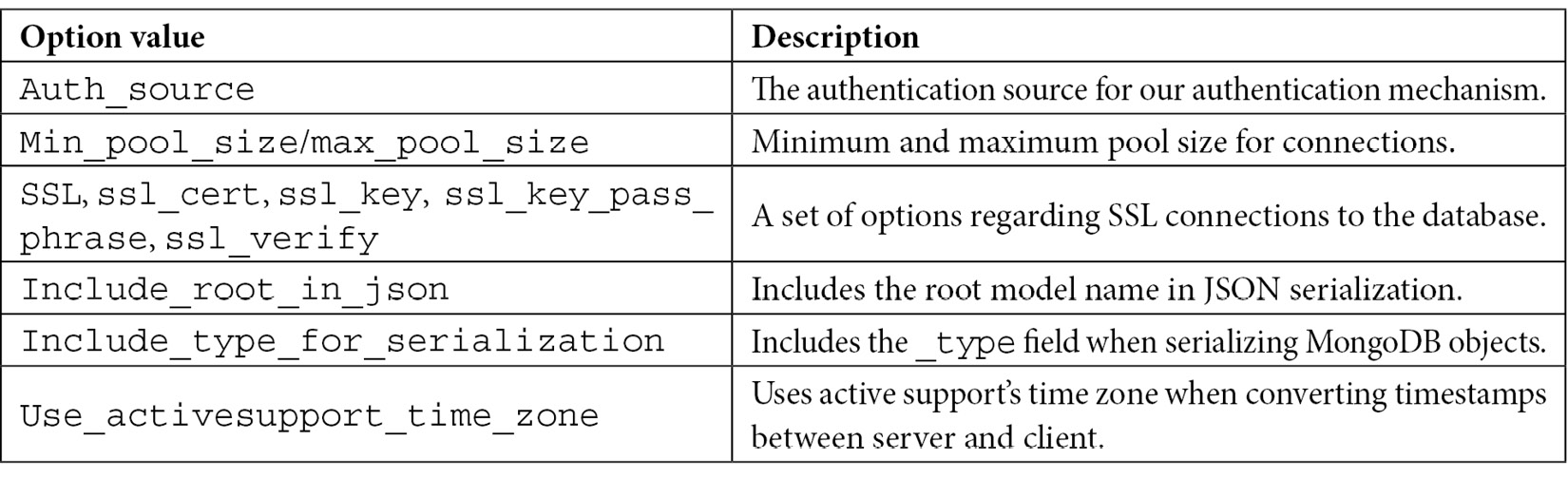
Table 2.2 – Mongoid configuration options
The next step is to modify our models to be stored in MongoDB. This is as simple as including one line of code in the model declaration, as shown in the following example:
class Person
include Mongoid::Document
End
We can also use the following code:
include Mongoid::Timestamps
We use it to generate created_at and updated_at fields in a similar way to Active Record. Data fields do not need to be declared by type in our models, but it’s good practice to do so. The supported data types are as follows:
- Array
- BigDecimal
- Boolean
- Date
- DateTime
- Float
- Hash
- Integer
- BSON::ObjectId
- BSON::Binary
- Range
- Regexp
- String
- Symbol
- Time
- TimeWithZone
If the types of fields are not defined, fields will be cast to the object and stored in the database. This is slightly faster but doesn’t support all types. If we try to use BigDecimal, Date, DateTime, or Range, we will get back an error.
Inheritance with Mongoid models
The following code is an example of inheritance using the Mongoid models:
class Canvas
include Mongoid::Document
field :name, type: String
embeds_many :shapes
end
class Shape
include Mongoid::Document
field :x, type: Integer
field :y, type: Integer
embedded_in :canvas
end
class Circle < Shape
field :radius, type: Float
end
class Rectangle < Shape
field :width, type: Float
field :height, type: Float
end
Now, we have a Canvas class with many Shape objects embedded in it. Mongoid will automatically create a field, which is _type, to distinguish between parent and child node fields. When a document is inherited from its fields, relationships, validations, and scopes will propagate down into the child document.
The opposite will not happen; embeds_many and embedded_in pairs will create embedded subdocuments to store the relationships. If we want to store these via referencing to ObjectId, we can do so by substituting these with has_many and belongs_to.
Connecting using Python
A strong contender to Ruby and Rails is Python and Django. Similar to Mongoid, there is MongoEngine and an official MongoDB low-level driver, PyMongo.
Installing PyMongo can be done using pip or easy_install, as shown in the following code:
python -m pip install pymongo
python -m easy_install pymongo
Then, in our class, we can connect to a database, as shown in the following example:
>>> from pymongo import MongoClient
>>> client = MongoClient()
Connecting to a replica set requires a set of seed servers for the client to find out what the primary, secondary, or arbiter nodes in the set are, as indicated in the following example:
client = pymongo.MongoClient('mongodb://user:passwd@node1:p1,node2:p2/?replicaSet=rsname')
Using the connection string URL, we can pass a username and password and the replicaSet name all in a single string. Some of the most interesting options for the connection string URL are presented in the next section.
Connecting to a shard requires the server host and IP for the MongoDB router, which is the MongoDB process.
PyMODM ODM
Similar to Ruby’s Mongoid, PyMODM is an ODM for Python that follows Django’s built-in ORM closely. Installing pymodm can be done via pip, as shown in the following code:
pip install pymodm
Then, we need to edit settings.py and replace the ENGINE database with a dummy database, as shown in the following code:
DATABASES = { 'default': {'ENGINE': 'django.db.backends.dummy'
}
}
Then we add our connection string anywhere in settings.py, as shown in the following code:
from pymodm import connect
connect("mongodb://localhost:27017/myDatabase", alias="MyApplication")Here, we have to use a connection string that has the following structure:
mongodb://[username:password@]host1[:port1][,host2[:port2],...[,hostN[:portN]]][/[database][?options]]
Options have to be pairs of name=value with an & between each pair. Some interesting pairs are shown in the following table:

Table 2.3 – PyMODM configuration options
Model classes need to inherit from MongoModel. The following code shows what a sample class will look like:
from pymodm import MongoModel, fields
class User(MongoModel):
email = fields.EmailField(primary_key=True)
first_name = fields.CharField()
last_name = fields.CharField()
This has a User class with first_name, last_name, and email fields, where email is the primary field.
Inheritance with PyMODM models
Handling one-to-one and one-to-many relationships in MongoDB can be done using references or embedding. The following example shows both ways, which are references for the model user and embedding for the comment model:
from pymodm import EmbeddedMongoModel, MongoModel, fields
class Comment(EmbeddedMongoModel):
author = fields.ReferenceField(User)
content = fields.CharField()
class Post(MongoModel):
title = fields.CharField()
author = fields.ReferenceField(User)
revised_on = fields.DateTimeField()
content = fields.CharField()
comments = fields.EmbeddedDocumentListField(Comment)
Similar to Mongoid for Ruby, we can define relationships as being embedded or referenced depending on our design decision.
Connecting using PHP
The MongoDB PHP driver was rewritten from scratch around five years ago to support the PHP 5, PHP 7, and HHVM architectures. The current architecture is shown in the following diagram:
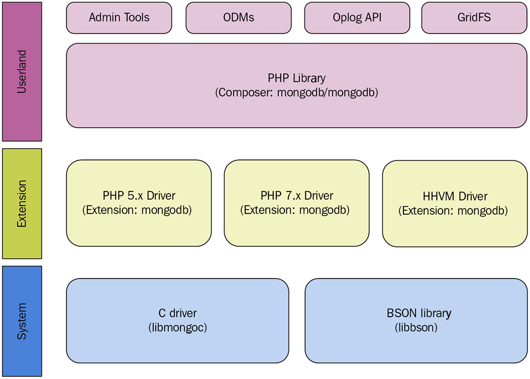
Figure 2.3 – PHP driver architecture
Currently, we have official drivers for all three architectures with full support for the underlying functionality.
Installation is a two-step process. The first step is to install the MongoDB extension. This extension is dependent on the version of PHP (or HHVM) that we have installed and can be done using brew in macOS. The following example is with PHP 7.0:
brew install php70-mongodb
Whereas this example uses PECL:
pecl install mongodb
Then, copy the following line and place it at the end of your php.ini file:
extension=mongodb.so
The php -i | grep mongodb output should then reference libmongoc and libmongocrypt.
The second step is to use composer (a widely-used dependency manager for PHP), as shown in the following example:
composer require mongodb/mongodb
Connecting to the database can be done by using the connection string URL or by passing an array of options.
Using the connection string URL, we have the following code:
$client = new MongoDBClient($uri = 'mongodb://127.0.0.1/', array $uriOptions = [], array $driverOptions = [])
For example, to connect to a replica set using SSL authentication, we use the following code:
$client = new MongoDBClient('mongodb://myUsername:[email protected],rs2.example.com/?ssl=true&replicaSet=myReplicaSet&authSource=admin');
Alternatively, we can use the $uriOptions parameter to pass in parameters without using the connection string URL, as shown in the following code:
$client = new MongoDBClient(
'mongodb://rs1.example.com,rs2.example.com/'
[
'username' => 'myUsername',
'password' => 'myPassword',
'ssl' => true,
'replicaSet' => 'myReplicaSet',
'authSource' => 'admin',
],
);
The $uriOptions set and the connection string URL options available are analogous to the ones used for Ruby and Python.
Doctrine ODM
Laravel is one of the most widely-used MVC frameworks for PHP, similar in architecture to Django and Rails, from the Python and Ruby worlds respectively. We will follow through with configuring our models using Laravel, Doctrine, and MongoDB. This section assumes that Doctrine is installed and working with Laravel 5.x.
Doctrine entities are Plain Old PHP Objects (POPO) that, unlike with Eloquent, Laravel’s default ORM doesn’t need to inherit from the Model class. Doctrine uses the data mapper pattern, whereas Eloquent uses Active Record. Skipping the get() and set() methods, a simple class would be shown in the following way:
use DoctrineORMMapping AS ORM;
use DoctrineCommonCollectionsArrayCollection;
/**
* @ORMEntity
* @ORMTable(name="scientist")
*/
class Scientist
{/**
* @ORMId
* @ORMGeneratedValue
* @ORMColumn(type="integer")
*/
protected $id;
/**
* @ORMColumn(type="string")
*/
protected $firstname;
/**
* @ORMColumn(type="string")
*/
protected $lastname;
/**
* @ORMOneToMany(targetEntity="Theory", mappedBy="scientist", cascade={"persist"})* @var ArrayCollection|Theory[]
*/
protected $theories;
/**
* @param $firstname
* @param $lastname
*/
public function __construct($firstname, $lastname)
{$this->firstname = $firstname;
$this->lastname = $lastname;
$this->theories = new ArrayCollection;
}
...
public function addTheory(Theory $theory)
{ if(!$this->theories->contains($theory)) {$theory->setScientist($this);
$this->theories->add($theory);
}
}
This POPO-based model uses annotations to define field types that need to be persisted in MongoDB. For example, @ORMColumn(type=”string”) defines a field in MongoDB, with the firstname and lastname string types as the attribute names in the respective lines.
There is a whole set of annotations available here: https://doctrine2.readthedocs.io/en/latest/reference/annotations-reference.html.
If we want to separate the POPO structure from annotations, we can also define them using YAML or XML instead of inlining them with annotations in our POPO model classes.
Inheritance with Doctrine
Modeling one-to-one and one-to-many relationships can be done via annotations, YAML, or XML. Using annotations, we can define multiple embedded subdocuments within our document, as shown in the following example:
/** @Document */
class User
{// ...
/** @EmbedMany(targetDocument="Phonenumber") */
private $phonenumbers = array();
// ...
}
/** @EmbeddedDocument */
class Phonenumber
{// ...
}
Here, a User document embeds many phone numbers. @EmbedOne() will embed one subdocument to be used for modeling one-to-one relationships.
Referencing is similar to embedding, as shown in the following example:
/** @Document */
class User
{// ...
/**
* @ReferenceMany(targetDocument="Account")
*/
private $accounts = array();
// ...
}
/** @Document */
class Account
{// ...
}
@ReferenceMany() and @ReferenceOne() are used to model one-to-many and one-to-one relationships via referencing into a separate collection.
Summary
In this chapter, we have learned about schema design for relational databases and MongoDB and how we can achieve the same goal starting from a different starting point.
In MongoDB, we have to think about read-write ratios, the questions that our users will have in the most common cases, and cardinality among relationships.
We have learned about atomic operations and how we can construct our queries so that we can have ACID properties without the overhead of transactions.
We have also learned about MongoDB data types, how they can be compared, and some special data types, such as ObjectId, which can be used both by the database and to our own advantage.
Starting from modeling simple one-to-one relationships, we have gone through one-to-many and also many-to-many relationship modeling, without the need for an intermediate table, as we would do in a relational database, either using references or embedded documents.
We have learned how to model data for keyword searches, one of the features that most applications need to support in a web context.
IoT is a rapidly evolving field and MongoDB provides special support for it. In this chapter, we have learned how to use time series collections to model and store sensor readings.
Finally, we have explored different use cases for using MongoDB with three of the most popular web programming languages. We saw examples using Ruby with the official driver and Mongoid ODM. Then, we explored how to connect using Python with the official driver and PyMODM ODM, and lastly, we worked through an example using PHP with the official driver and Doctrine ODM.
With all these languages (and many others), there are both official drivers offering support and full access functionality to the underlying database operations and also object data modeling frameworks, for ease of modeling our data and rapid development.
In the next chapter, we will dive deeper into the MongoDB shell and the operations we can achieve using it. We will also master using the drivers for CRUD operations on our documents.