
In this chapter we will develop the theory for binary decision trees. Decision trees can be used to classify data. Binary trees are the easiest to implement. We will create functions for the decision trees and to generate sets of data to classify.
8.1 Generate Classification Test Data
8.1.1 Problem
We want to generate a set of training and testing data.
8.1.2 Solution
Write a function using rand to generate data.
8.1.3 How It Works
The function ClassifierSet generates random data and assigns them to classes. Classes are generated by adding polygons that encompass the data. Any polygon can be used. The function randomly places points on a grid and then adds boundaries for the sets defined by polygons. You specify a set of vertices to be used in the set boundaries and the faces that define the set. The following code generates the sets:
function p = ClassifierSets( n, xRange, yRange, name, v, f, setName )
% Demo
if( nargin < 1 )
v = [0 0;0 4; 4 4; 4 0; 0 2; 2 2; 2 0;2 1;4 1;2 1];
f = {[5 6 7 1] [5 2 3 9 10 6] [7 8 9 4]};
ClassifierSets( 5, [0 4], [0 4], {’width’, ’length’}, v, f );
return
end
if( nargin < 7 )
setName = ’Classifier␣Sets’;
end
p.x = (xRange(2) - xRange(1))*(rand(n,n)-0.5) + mean(xRange);
p.y = (yRange(2) - yRange(1))*(rand(n,n)-0.5) + mean(yRange);
p.m = Membership( p, v, f );
NewFigure(setName);
m = length(f);
c = rand(m,3);
for k = 1:n
for j = 1:n
plot(p.x(k,j),p.y(k,j),’marker’,’o’,’MarkerEdgeColor’,’k’)
hold on
end
end
for k = 1:m
patch(’vertices’,v,’faces’,f{k},’facecolor’,c(k,:),’facealpha’,0.1)
end
xlabel(name{1});
ylabel(name{2});
grid
function z = Membership( p, v, f )
n = size(p.x,1);
m = size(p.x,2);
z = zeros(n,m);
for k = 1:n
for j = 1:m
for i = 1:length(f)
vI = v(f{i},:)’;
q = [p.x(k,j) p.y(k,j)];
r = PointInPolygon( q, vI );
if( r == 1 )
z(k,j) = i;
break;
end
end
end
end
A typical set is shown in Figure 8.1. The function color-codes the points to match the set color. Note that the colors are chosen randomly. The patch function is used to generate the polygons. The code shows a range of graphics coding including the use of graphics parameters.

Figure 8.1 Classifier set.
This function can generate test sets or demonstrate the trained decision tree. The drawing shows that the classification regions are boxes. ClassifierSets randomly puts points in the regions. It figures out which region each point is in using this code in the function:
function r = PointInPolygon( p, v )
m = size(v,2);
% All outside
r = 0;
% Put the first point at the end to simplify the looping
v = [v v(:,1)];
for i = 1:m
j = i + 1;
v2J = v(2,j);
v2I = v(2,i);
if (((v2I > p(2)) ~= (v2J > p(2))) && ...
(p(1) < (v(1,j) - v(1,i)) * (p(2) - v2I) / (v2J - v2I) + v(1,i)))
r = ~r;
end
end
This code can determine if a point is inside a polygon defined by a set of vertices. It is used frequently in computer graphics and in games when you need to know if one object’s vertex is in another polygon. You could correctly argue that this could replace our decision tree for this type of problem. However, a decision tree can compute membership for more complex sets of data. Our classifier set is simple and makes it easy to validate the results.
8.2 Drawing Decision Trees
8.2.1 Problem
We want to draw a binary decision tree to show decision tree thinking.
8.2.2 Solution
The solution is to use MATLAB graphics functions to draw a tree.
8.2.3 How It Works
The function DrawBinaryTree draws any binary tree. You pass it a data structure with the decision criteria in a cell array. The boxes start from the left and go row by row. In a binary tree the number of rows is related to the number of boxes through the formula for a geometric series: ![]() (8.1)
(8.1)
where m is the number of rows and n is the number of boxes. Therefore, the function can compute the number of rows.
The function starts by checking the number of inputs and either runs the demo or returns the default data structure. The name input is optional. It then steps through the boxes assigning them to rows based on it being a binary tree. The first row has one box, the next two boxes, the following four boxes, etc. As this is a geometric series, it will soon get unmanageable! This points to a problem with decision trees. If they have a depth of more than four, even drawing them is impossible.
As it draws the boxes it computes the bottom and top points that will be the anchors for the lines between the boxes. After drawing all the boxes it draws all the lines.
All of the drawing functionality is in the subfunction DrawBoxes. This draws a box using the patch function and the text using the text function. Notice the extra arguments in text. The most interesting is ’HorizontalAlignment’. This allows you to easily center text in the box.
text(x+w/2,y + h/2,t,’fontname’,d.font,’fontsize’,d.fontSize,
’HorizontalAlignment’,’center’);
Setting ’facecolor’ to [ 1 1 1] makes the face white and leaves the edges black. As with all MATLAB graphics there are dozens of properties that you can edit to produce beautiful graphics. The following listing shows the code.
%% DRAWBINARYTREE - Draw a binary tree in a new figure
%% Forms:
% DrawBinaryTree( d, name )
% d = DrawBinaryTree % default data structure
%
%% Description
% Draws a binary tree. All branches are drawn. Inputs in d.box go from left
% to right by row starting with the row with only one box.
%
%% Inputs
% d (.) Data structure
% .w (1,1) Box width
% .h (1,1) Box height
% .rows (1,1) Number of rows in the tree
% .fontSize (1,1) Font size
% .font (1,:) Font name
% .box {:} Text for each box
% name (1,:) Figure name
%
%% Outputs
% d (.) Data structure
function d = DrawBinaryTree( d, name )
% Demo
if( nargin < 1 )
if( nargout == 0 )
Demo
else
d = DefaultDataStructure;
end
return
end
if( nargin < 2 )
name = ’Binary␣Tree’;
end
NewFigure(name);
m = length(d.box);
nRows = ceil(log2(m+1));
w = d.w;
h = d.h;
i = 1;
x = -w/2;
y = 1.5*nRows*h;
nBoxes = 1;
bottom = zeros(m,2);
top = zeros(m,2);
rowID = cell(nRows,1);
for k = 1:nRows
for j = 1:nBoxes
bottom(i,:) = [x+w/2 y ];
top(i,:) = [x+w/2 y+h];
DrawBox(d.box{i},x,y,w,h,d);
rowID{k} = [rowID{k} i];
i = i + 1;
x = x + 1.5*w;
if( i > length(d.box) )
break;
end
end
nBoxes = 2*nBoxes;
x = -(0.25+0.5*(nBoxes/2-1))*w - nBoxes*w/2;
y = y - 1.5*h;
end
% Draw the lines
for k = 1:length(rowID)-1
iD = rowID{k};
i0 = 0;
% Work from left to right of the current row
for j = 1:length(iD)
x(1) = bottom(iD(j),1);
y(1) = bottom(iD(j),2);
iDT = rowID{k+1};
if( i0+1 > length(iDT) )
break;
end
for i = 1:2
x(2) = top(iDT(i0+i),1);
y(2) = top(iDT(i0+i),2);
line(x,y);
end
i0 = i0 + 2;
end
end
axis off
function DrawBox( t, x, y, w, h, d )
%% Draw boxes and text
v = [x y 0;x y+h 0; x+w y+h 0;x+w y 0];
patch(’vertices’,v,’faces’,[1 2 3 4],’facecolor’,[1;1;1]);
text(x+w/2,y + h/2,t,’fontname’,d.font,’fontsize’,d.fontSize,’HorizontalAlignment’,’center’);
function d = DefaultDataStructure
%% Default data structure
d = struct();
d.fontSize = 12;
d.font = ’courier’;
d.w = 1;
d.h = 0.5;
d.box = {};
function Demo
%% Demo
d = DefaultDataStructure;
d.box{1} = ’a␣>␣0.1’;
d.box{2} = ’b␣>␣0.2’;
d.box{3} = ’b␣>␣0.3’;
d.box{4} = ’a␣>␣0.8’;
d.box{5} = ’b␣>␣0.4’;
d.box{6} = ’a␣>␣0.2’;
d.box{7} = ’b␣>␣0.3’;
DrawBinaryTree( d );
The demo creates three rows. It starts with the default data structure. You only have to add strings for the decision points. You can create them using sprintf. For example, for the first box you could write
s = sprintf(’%s␣%s␣%3.1f’,’a’,’>’,0.1);
The relationship could be added with an if-else-end construct. You can see this done in DecisionTree. The following demo draws a binary tree:
d.box = {};
function Demo
%% Demo
d = DefaultDataStructure;
d.box{1} = ’a␣>␣0.1’;
d.box{2} = ’b␣>␣0.2’;
d.box{3} = ’b␣>␣0.3’;
d.box{4} = ’a␣>␣0.8’;
d.box{5} = ’b␣>␣0.4’;
d.box{6} = ’a␣>␣0.2’;
d.box{7} = ’b␣>␣0.3’;
The binary tree resulting from the demo is shown in Figure 8.2. The text in the boxes could be anything you want.

Figure 8.2 Binary tree
8.3 Decision Tree Implementation
Decision trees are the main focus of this chapter. We’ll start by looking at how we determine if our decision tree is working correctly. We’ll then hand-build a decision tree and finally write learning code to generate the decisions for each block of the tree.
8.3.1 Problem
We need to measure the homogeneity of a set of data at different nodes on the decision tree.
8.3.2 Solution
The solution is to implement the Gini impurity measure for a set of data.
8.3.3 How It Works
The homogeneity measure is called the information gain (IG).
The IG is defined as the increase in information by splitting at the node. This is  (8.2)
(8.2)
where I is the impurity measure and N is the number of samples at that node. If our tree is working it should go down, eventually to zero or to a very small number. In our training set we know the class of each data point. Therefore, we can determine the IG. Essentially, we have gained information if the mixing decreases in the child nodes. For example, in the first node all the data are mixed. In the two child nodes we expect that each child node will have more of one class than does the other child node. Essentially, we look at the percentages of classes in each node and look for the maximum increase in nonhomogeneity.
There are three impurity measures:
Gini impurity
Entropy
Classification error
The Gini impurity is the criterion to minimize the probability of misclassification. We don’t want to push a sample into the wrong category.  (8.3)
(8.3)
p(i | t) is the proportion of the samples in class c
i
at node t. For a binary class, entropy is either zero or one.  (8.4)
(8.4)
The classification error is ![]() (8.5) We will use the Gini impurity in the decision tree. The following code implements the Gini measure.
(8.5) We will use the Gini impurity in the decision tree. The following code implements the Gini measure.
function [i, d] = HomogeneityMeasure( action, d, data )
if( nargin == 0 )
if( nargout == 1 )
i = DefaultDataStructure;
else
Demo;
end
return
end
switch lower(action)
case ’initialize’
d = Initialize( d, data );
i = d.i;
case ’update’
d = Update( d, data );
i = d.i;
otherwise
error(’%s␣is␣not␣an␣available␣action’,action);
end
function d = Update( d, data )
%% Update
newDist = zeros(1,length(d.class));
m = reshape(data,[],1);
c = d.class;
n = length(m);
if( n > 0 )
for k = 1:length(d.class)
j = find(m==d.class(k));
newDist(k) = length(j)/n;
end
end
d.i = 1 - sum(newDist.^2);
d.dist = newDist;
function d = Initialize( d, data )
%% Initialize
m = reshape(data,[],1);
c = 1:max(m);
n = length(m);
d.dist = zeros(1,c(4));
d.class = c;
if( n > 0 )
for k = 1:length(c)
j = find(m==c(k));
d.dist(k) = length(j)/n;
end
end
d.i = 1 - sum(d.dist.^2);
function d = DefaultDataStructure
%% Default data structure
d.dist = [];
d.data = [];
d.class = [];
d.i = 1;
The demo is shown below.
function d = Demo
%% Demo
data = [ 1 2 3 4 3 1 2 4 4 1 1 1 2 2 3 4]’;
d = HomogeneityMeasure;
[i, d] = HomogeneityMeasure( ’initialize’, d, data )
data = [1 1 1 2 2];
[i, d] = HomogeneityMeasure( ’update’, d, data )
data = [1 1 1 1];
[i, d] = HomogeneityMeasure( ’update’, d, data )
data = [];
[i, d] = HomogeneityMeasure( ’update’, d, data )
>> HomogeneityMeasure
i =
0.7422
d =
dist: [0.3125 0.2500 0.1875 0.2500]
data: []
class: [1 2 3 4]
i: 0.7422
i =
0.4800
d =
dist: [0.6000 0.4000 0 0]
data: []
class: [1 2 3 4]
i: 0.4800
i =
0
d =
dist: [1 0 0 0]
data: []
class: [1 2 3 4]
i: 0
i =
1
d =
dist: [0 0 0 0]
data: []
class: [1 2 3 4]
i: 1
The second-to-last set has a zero, which is the desired value. If there are no inputs, it returns 1 since by definition for a class to exist it must have members.
8.4 Implementing a Decision Tree
8.4.1 Problem
We want to implement a decision tree for classifying data.
8.4.2 Solution
The solution is to write a binary decision tree function in MATLAB.
8.4.3 How It Works
A decision tree [1] breaks down data by asking a series of questions about the data. Our decision trees will be binary in that there will a yes or no answer to each question. For each feature in the data we ask one question per node. This always splits the data into two child nodes. We will be looking at two parameters that determine class membership. The parameters will be numerical measurements.
At the following nodes we ask additional questions, further splitting the data. Figure 8.3 shows the parent/child structure.

Figure 8.3 Parent/child nodes.
We continue this process until the samples at each node are in one of the classes. At each node we want to ask the question that provides us with the most information about which class in which our samples reside.
In constructing our decision tree for a two-parameter classification we have two decisions at each node:
Which parameter to check
What level to check
For example, for our two parameters we would have either ![]() (8.6)
(8.6)
![]() (8.7) This can be understood with a very simple case. Suppose we have four sets in a two-dimensional space divided by one horizontal and one vertical line. Our sets can be generated with the following code.
(8.7) This can be understood with a very simple case. Suppose we have four sets in a two-dimensional space divided by one horizontal and one vertical line. Our sets can be generated with the following code.
This is done using the Gini values given above. We use fminbnd at each node, once for each of the two parameters. There are two actions, ”train” and ”test.” ”train” creates the decision tree and ”test” runs the generated decision tree. You an also input your own decision tree. FindOptimalAction finds the parameter that minimizes the inhomogeneity on both sides of the division. The function called by fminbnd is RHSGT. We only implement the greater-than action.
The structure of the testing function is very similar to the training function.
%% DECISIONTREE - implements a decision tree
%% Form
% [d, r] = DecisionTree( action, d, t )
%
%% Description
% Implements a binary classification tree.
% Type DecisionTree for a demo using the SimpleClassifierExample
%
%% Inputs
% action (1,:) Action ’train’, ’test’
% d (.) Data structure
% t {:} Inputs for training or testing
%
%% Outputs
% d (.) Data structure
% r (:) Results
%
%% References
% None
function [d, r] = DecisionTree( action, d, t )
if( nargin < 1 )
if( nargout > 0 )
d = DefaultDataStructure;
else
Demo;
end
return
end
switch lower(action)
case ’train’
d = Training( d, t );
case ’test’
for k = 1:length(d.box)
d.box(k).id = [];
end
[r, d] = Testing( d, t );
otherwise
error(’%s␣is␣not␣an␣available␣action’,action);
end
function d = Training( d, t )
%% Training function
[n,m] = size(t.x);
nClass = max(t.m);
box(1) = AddBox( 1, 1:n*m, [] );
box(1).child = [2 3];
[~, dH] = HomogeneityMeasure( ’initialize’, d, t.m );
class = 0;
nRow = 1;
kR0 = 0;
kNR0 = 1; % Next row;
kInRow = 1;
kInNRow = 1;
while( class < nClass )
k = kR0 + kInRow;
idK = box(k).id;
if( isempty(box(k).class) )
[action, param, val, cMin] = FindOptimalAction( t, idK, d.xLim, d.yLim, dH );
box(k).value = val;
box(k).param = param;
box(k).action = action;
x = t.x(idK);
y = t.y(idK);
if( box(k).param == 1 ) % x
id = find(x > d.box(k).value );
idX = find(x <= d.box(k).value );
else % y
id = find(y > d.box(k).value );
idX = find(y <= d.box(k).value );
end
% Child boxes
if( cMin < d.cMin)
class = class + 1;
kN = kNR0 + kInNRow;
box(k).child = [kN kN+1];
box(kN) = AddBox( kN, idK(id), class );
class = class + 1;
kInNRow = kInNRow + 1;
kN = kNR0 + kInNRow;
box(kN) = AddBox( kN, idK(idX), class );
kInNRow = kInNRow + 1;
else
kN = kNR0 + kInNRow;
box(k).child = [kN kN+1];
box(kN) = AddBox( kN, idK(id) );
kInNRow = kInNRow + 1;
kN = kNR0 + kInNRow;
box(kN) = AddBox( kN, idK(idX) );
kInNRow = kInNRow + 1;
end
% Update current row
kInRow = kInRow + 1;
if( kInRow > nRow )
kR0 = kR0 + nRow;
nRow = 2*nRow;
kNR0 = kNR0 + nRow;
kInRow = 1;
kInNRow = 1;
end
end
end
for k = 1:length(box)
if( ~isempty(box(k).class) )
box(k).child = [];
end
box(k).id = [];
fprintf(1,’Box␣%d␣action␣%s␣Value␣%4.1f␣%d ’,k,box(k).action,box(k).value,ischar(box(k).action));
end
d.box = box;
function [action, param, val, cMin] = FindOptimalAction( t, iD, xLim, yLim, dH )
c = zeros(1,2);
v = zeros(1,2);
x = t.x(iD);
y = t.y(iD);
m = t.m(iD);
[v(1),c(1)] = fminbnd( @RHSGT, xLim(1), xLim(2), optimset(’TolX’,1e-16), x, m, dH );
[v(2),c(2)] = fminbnd( @RHSGT, yLim(1), yLim(2), optimset(’TolX’,1e-16), y, m, dH );
% Find the minimum
[cMin, j] = min(c);
action = ’>’;
param = j;
val = v(j);
function q = RHSGT( v, u, m, dH )
%% RHS greater than function for fminbnd
j = find( u > v );
q1 = HomogeneityMeasure( ’update’, dH, m(j) );
j = find( u <= v );
q2 = HomogeneityMeasure( ’update’, dH, m(j) );
q = q1 + q2;
function [r, d] = Testing( d, t )
%% Testing function
k = 1;
[n,m] = size(t.x);
d.box(1).id = 1:n*m;
class = 0;
while( k <= length(d.box) )
idK = d.box(k).id;
v = d.box(k).value;
switch( d.box(k).action )
case ’>’
if( d.box(k).param == 1 )
id = find(t.x(idK) > v );
idX = find(t.x(idK) <= v );
else
id = find(t.y(idK) > v );
idX = find(t.y(idK) <= v );
end
d.box(d.box(k).child(1)).id = idK(id);
d.box(d.box(k).child(2)).id = idK(idX);
case ’<=’
if( d.box(k).param == 1 )
id = find(t.x(idK) <= v );
idX = find(t.x(idK) > v );
else
id = find(t.y(idK) <= v );
idX = find(t.y(idK) > v );
end
d.box(d.box(k).child(1)).id = idK(id);
d.box(d.box(k).child(2)).id = idK(idX);
otherwise
class = class + 1;
d.box(k).class = class;
end
k = k + 1;
end
r = cell(class,1);
for k = 1:length(d.box)
if( ~isempty(d.box(k).class) )
r{d.box(k).class,1} = d.box(k).id;
end
end
8.5 Creating a Hand-Made Decision Tree
8.5.1 Problem
We want to test a hand-made decision tree.
8.5.2 Solution
The solution is to write script to test a hand-made decision tree.
8.5.3 How It Works
We write the test script shown below. It uses the ’test’ action for DecisionTree.
% Create the decision tree
d = DecisionTree;
% Vertices for the sets
v = [ 0 0; 0 4; 4 4; 4 0; 2 4; 2 2; 2 0; 0 2; 4 2];
% Faces for the sets
f = { [6 5 2 8] [6 7 4 9] [6 9 3 5] [1 7 6 8] };
% Generate the testing set
pTest = ClassifierSets( 5, [0 4], [0 4], {’width’, ’length’}, v, f, ’Testing␣Set’ );
% Test the tree
[d, r] = DecisionTree( ’test’, d, pTest );
q = DrawBinaryTree;
c = ’xy’;
for k = 1:length(d.box)
if( ~isempty(d.box(k).action) )
q.box{k} = sprintf(’%c␣%s␣%4.1f’,c(d.box(k).param),d.box(k).action,d.box(k).value);
else
q.box{k} = sprintf(’Class␣%d’,d.box(k).class);
end
end
DrawBinaryTree(q);
m = reshape(pTest.m,[],1);
for k = 1:length(r)
fprintf(1,’Class␣%d ’,k);
for j = 1:length(r{k})
fprintf(1,’%d:␣%d ’,r{k}(j),m(r{k}(j)));
end
end
SimpleClassifierDemo uses the hand-built example in DecisionTree.
kN = kNR0 + kInNRow;
box(kN) = AddBox( kN, idK(idX) );
kInNRow = kInNRow + 1;
end
% Update current row
kInRow = kInRow + 1;
if( kInRow > nRow )
kR0 = kR0 + nRow;
nRow = 2*nRow;
kNR0 = kNR0 + nRow;
kInRow = 1;
kInNRow = 1;
end
end
end
for k = 1:length(box)
if( ~isempty(box(k).class) )
box(k).child = [];
end
box(k).id = [];
fprintf(1,’Box␣%d␣action␣%s␣Value␣%4.1f␣%d ’,k,box(k).action,box(k).value,ischar(box(k).action));
end
d.box = box;
function [action, param, val, cMin] = FindOptimalAction( t, iD, xLim, yLim, dH )
c = zeros(1,2);
v = zeros(1,2);
x = t.x(iD);
y = t.y(iD);
m = t.m(iD);
[v(1),c(1)] = fminbnd( @RHSGT, xLim(1), xLim(2), optimset(’TolX’,1e-16), x, m, dH );
[v(2),c(2)] = fminbnd( @RHSGT, yLim(1), yLim(2), optimset(’TolX’,1e-16), y, m, dH );
% Find the minimum
[cMin, j] = min(c);
action = ’>’;
param = j;
val = v(j);
function q = RHSGT( v, u, m, dH )
%% RHS greater than function for fminbnd
j = find( u > v );
q1 = HomogeneityMeasure( ’update’, dH, m(j) );
j = find( u <= v );
q2 = HomogeneityMeasure( ’update’, dH, m(j) );
The action for the last four box fields as empty strings. This means that no further operations are performed. This happens in the last boxes in the decision tree. In those boxes the class field will contain the class of that box. The following shows the testing function in DecisionTree.
function [r, d] = Testing( d, t )
%% Testing function
k = 1;
[n,m] = size(t.x);
d.box(1).id = 1:n*m;
class = 0;
while( k <= length(d.box) )
idK = d.box(k).id;
v = d.box(k).value;
switch( d.box(k).action )
case ’>’
if( d.box(k).param == 1 )
id = find(t.x(idK) > v );
idX = find(t.x(idK) <= v );
else
id = find(t.y(idK) > v );
idX = find(t.y(idK) <= v );
end
d.box(d.box(k).child(1)).id = idK(id);
d.box(d.box(k).child(2)).id = idK(idX);
case ’<=’
if( d.box(k).param == 1 )
id = find(t.x(idK) <= v );
idX = find(t.x(idK) > v );
else
id = find(t.y(idK) <= v );
idX = find(t.y(idK) > v );
end
d.box(d.box(k).child(1)).id = idK(id);
d.box(d.box(k).child(2)).id = idK(idX);
otherwise
class = class + 1;
d.box(k).class = class;
end
k = k + 1;
end
r = cell(class,1);
for k = 1:length(d.box)
if( ~isempty(d.box(k).class) )
r{d.box(k).class,1} = d.box(k).id;
end
end
Figure 8.4 shows the results. There are four rectangular areas, which are our sets.

Figure 8.4 Data and classes in the test set.
We can create a decision tree by hand as shown Figure 8.5.

Figure 8.5 A manually created decision tree. The drawing is generated by DecisionTree. The last row of boxes is the data sorted into the four classes.
The decision tree sorts the samples into the four sets. In this case we know the boundaries and can use them to write the inequalities. In software we will have to determine what values provide the shortest branches. The following is the output. The decision tree properly classifies all of the data.
>> SimpleClassifierDemo
Class 1
7: 3
9: 3
13: 3
15: 3
Class 2
2: 2
3: 2
11: 2
14: 2
16: 2
17: 2
21: 2
23: 2
25: 2
Class 3
4: 1
8: 1
10: 1
12: 1
18: 1
19: 1
20: 1
22: 1
Class 4
1: 4
5: 4
6: 4
24: 4
The class numbers and numbers in the list aren’t necessarily the same since the function does know the names of the classes.
8.6 Training and Testing the Decision Tree
8.6.1 Problem
We want to train our decision tree and test the results.
8.6.2 Solution
We replicated the previous recipe only this time we have DecisionTree create the decision tree.
8.6.3 How It Works
The following script trains and tests the decision tree. It is very similar to the code for the hand-built decision tree.
% Vertices for the sets
v = [ 0 0; 0 4; 4 4; 4 0; 2 4; 2 2; 2 0; 0 2; 4 2];
% Faces for the sets
f = { [6 5 2 8] [6 7 4 9] [6 9 3 5] [1 7 6 8] };
% Generate the training set
pTrain = ClassifierSets( 40, [0 4], [0 4], {’width’, ’length’}, v, f, ’Training␣Set’ );
% Create the decision tree
d = DecisionTree;
d = DecisionTree( ’train’, d, pTrain );
% Generate the testing set
pTest = ClassifierSets( 5, [0 4], [0 4], {’width’, ’length’}, v, f, ’Testing␣Set’ );
% Test the tree
[d, r] = DecisionTree( ’test’, d, pTest );
q = DrawBinaryTree;
c = ’xy’;
for k = 1:length(d.box)
if( ~isempty(d.box(k).action) )
q.box{k} = sprintf(’%c␣%s␣%4.1f’,c(d.box(k).param),d.box(k).action,d.box(k).value);
else
q.box{k} = sprintf(’Class␣%d’,d.box(k).class);
end
end
DrawBinaryTree(q);
m = reshape(pTest.m,[],1);
for k = 1:length(r)
fprintf(1,’Class␣%d ’,k);
for j = 1:length(r{k})
fprintf(1,’%d:␣%d ’,r{k}(j),m(r{k}(j)));
end
end
It uses ClassifierSets to generate the training data. The output includes the coordinates and the sets in which they fall. We then create the default data structure and call DecisionTree in training mode. The training takes place in this code:
function d = Training( d, t )
%% Training function
[n,m] = size(t.x);
nClass = max(t.m);
box(1) = AddBox( 1, 1:n*m, [] );
box(1).child = [2 3];
[~, dH] = HomogeneityMeasure( ’initialize’, d, t.m );
class = 0;
nRow = 1;
kR0 = 0;
kNR0 = 1; % Next row;
kInRow = 1;
kInNRow = 1;
while( class < nClass )
k = kR0 + kInRow;
idK = box(k).id;
if( isempty(box(k).class) )
[action, param, val, cMin] = FindOptimalAction( t, idK, d.xLim, d.yLim, dH );
box(k).value = val;
box(k).param = param;
box(k).action = action;
x = t.x(idK);
y = t.y(idK);
if( box(k).param == 1 ) % x
id = find(x > d.box(k).value );
idX = find(x <= d.box(k).value );
else % y
id = find(y > d.box(k).value );
idX = find(y <= d.box(k).value );
end
% Child boxes
if( cMin < d.cMin)
class = class + 1;
kN = kNR0 + kInNRow;
box(k).child = [kN kN+1];
box(kN) = AddBox( kN, idK(id), class );
class = class + 1;
kInNRow = kInNRow + 1;
kN = kNR0 + kInNRow;
box(kN) = AddBox( kN, idK(idX), class );
kInNRow = kInNRow + 1;
else
kN = kNR0 + kInNRow;
box(k).child = [kN kN+1];
box(kN) = AddBox( kN, idK(id) );
kInNRow = kInNRow + 1;
kN = kNR0 + kInNRow;
box(kN) = AddBox( kN, idK(idX) );
kInNRow = kInNRow + 1;
end
% Update current row
kInRow = kInRow + 1;
if( kInRow > nRow )
kR0 = kR0 + nRow;
nRow = 2*nRow;
kNR0 = kNR0 + nRow;
kInRow = 1;
kInNRow = 1;
end
end
end
for k = 1:length(box)
if( ~isempty(box(k).class) )
box(k).child = [];
end
box(k).id = [];
fprintf(1,’Box␣%d␣action␣%s␣Value␣%4.1f␣%d ’,k,box(k).action,box(k).value,ischar(box(k).action));
end
d.box = box;
function [action, param, val, cMin] = FindOptimalAction( t, iD, xLim, yLim, dH )
c = zeros(1,2);
v = zeros(1,2);
x = t.x(iD);
y = t.y(iD);
m = t.m(iD);
[v(1),c(1)] = fminbnd( @RHSGT, xLim(1), xLim(2), optimset(’TolX’,1e-16), x, m, dH );
[v(2),c(2)] = fminbnd( @RHSGT, yLim(1), yLim(2), optimset(’TolX’,1e-16), y, m, dH );
% Find the minimum
[cMin, j] = min(c);
action = ’>’;
param = j;
val = v(j);
function q = RHSGT( v, u, m, dH )
%% RHS greater than function for fminbnd
j = find( u > v );
q1 = HomogeneityMeasure( ’update’, dH, m(j) );
j = find( u <= v );
q2 = HomogeneityMeasure( ’update’, dH, m(j) );
q = q1 + q2;
We use fminbnd to find the optimal switch point. We need to compute the homogeneity on both sides of the switch and sum the values. The sum is minimized by fminbnd. This code is designed for rectangular region classes. Other boundaries won’t necessarily work correctly. The code is fairly involved. It needs to keep track of the box numbering to make the parent/child connections. When the homogeneity measure is low enough, it marks the boxes as containing the classes.
The tree is shown in Figure 8.8. The training data are shown in Figure 8.6 and the testing data in Figure 8.7. We need enough testing data to fill the classes. Otherwise, the decision tree generator may draw the lines to encompass just the data in the training set.
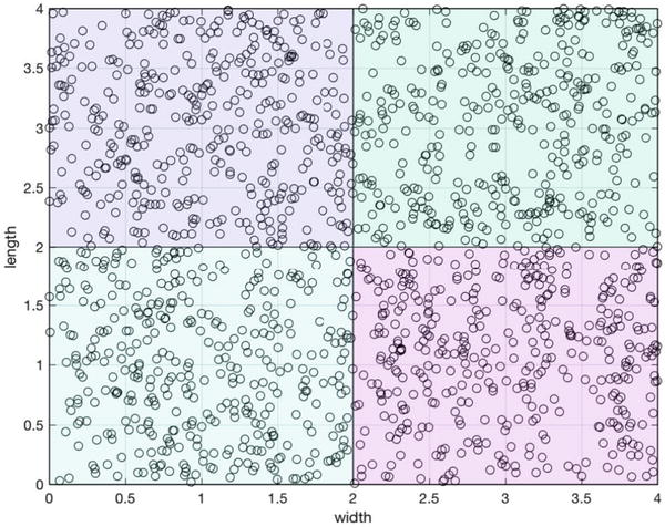
Figure 8.6 The training data. A large amount of data is needed to fill the classes.

Figure 8.7 The testing data.

Figure 8.8 The tree derived from the training data. It is essentially the same as the hand-derived tree. The values in the generated tree are not exactly 2.0.
The results are similar to the simple test.
Class 1
2: 3
7: 3
9: 3
10: 3
18: 3
19: 3
Class 2
6: 2
11: 2
20: 2
22: 2
24: 2
25: 2
Class 3
3: 1
5: 1
8: 1
12: 1
13: 1
14: 1
21: 1
23: 1
Class 4
1: 4
4: 4
15: 4
16: 4
17: 4
The generated tree separates the data effectively.
Summary
This chapter has demonstrated data classification using decision trees in MATLAB. We also wrote a new graphics function to draw decision trees. The decision tree software is not general purpose but can serve as a guide to more general-purpose code. Table 8.1 summarizes the code listings from the chapter.
Table 8.1 Chapter Code Listing
File | Description |
ClassifierSets | Generates data for classification or training |
DecisionTree | Implements a decision tree to classify data |
DrawBinaryTree | Generates data for classification or training |
HomogeneityMeasure | Computes Gini impurity |
SimpleClassifierDemo | Demonstrates decision tree testing |
SimpleClassifierExample | Generates data for a simple problem |
TestDecisionTree | Tests a decision tree |
[1] Sebastian Raschka. Python Machine Learning. [PACKT], 2015.