Chapter 9. Tuples, Files, and Everything Else
This chapter rounds out our in-depth look at the core object types in Python by exploring the tuple (a collection of other objects that cannot be changed), and the file (an interface to external files on your computer). As you’ll see, the tuple is a relatively simple object that largely performs operations you’ve already learned about for strings and lists. The file object is a commonly used and full-featured tool for processing files; the basic overview of files here will be supplemented by further file examples that appear in later chapters of this book.
This chapter also concludes this part of the book by looking at properties common to all the core object types we’ve met—the notions of equality, comparisons, object copies, and so on. We’ll also briefly explore other object types in the Python toolbox; as you’ll see, although we’ve covered all the primary built-in types, the object story in Python is broader than I’ve implied thus far. Finally, we’ll close this part of the book by taking a look at a set of common object type pitfalls, and exploring some exercises that will allow you to experiment with the ideas you’ve learned.
Tuples
The last collection type in our survey is the Python tuple. Tuples construct simple groups of objects. They work exactly like lists, except that tuples can’t be changed in-place (they’re immutable), and are usually written as a series of items in parentheses, not square brackets. Although they don’t support any method calls, tuples share most of their properties with lists. Here’s a quick look at their properties. Tuples are:
- Ordered collections of arbitrary objects
Like strings and lists, tuples are positionally ordered collections of objects (i.e., they maintain a left-to-right order among their contents); like lists, they can embed any kind of object.
- Accessed by offset
Like strings and lists, items in a tuple are accessed by offset (not by key); they support all the offset-based access operations, such as indexing and slicing.
- Of the category immutable sequence
Like strings, tuples are immutable; they don’t support any of the in-place change operations applied to lists. Like strings and lists, tuples are sequences; they support many of the same operations.
- Fixed-length, heterogeneous, and arbitrarily nestable
Because tuples are immutable, you cannot change their size without making a copy. On the other hand, tuples can hold other compound objects (e.g., lists, dictionaries, other tuples), and so support arbitrary nesting.
- Arrays of object references
Like lists, tuples are best thought of as object reference arrays; tuples store access points to other objects (references), and indexing a tuple is relatively quick.
Table 9-1 highlights common tuple operations. A tuple is written as a series of objects (technically, expressions that generate objects), separated by commas and enclosed in parentheses. An empty tuple is just a parentheses pair with nothing inside.
|
Operation |
Interpretation |
|
|
An empty tuple |
|
|
A one-item tuple (not an expression) |
|
|
A four-item tuple |
|
|
Another four-item tuple (same as prior line) |
|
|
Nested tuples |
|
|
Index, index of index, slice, length |
|
|
Concatenate, repeat |
|
|
Iteration, membership |
Tuples in Action
As usual, let’s start an interactive session to explore tuples at
work. Notice in Table 9-1
that tuples have no methods (e.g., an append call won’t work here). They do,
however, support the usual sequence operations that we saw for strings
and lists:
>>>
(1, 2) + (3, 4)# Concatenation (1, 2, 3, 4) >>>(1, 2) * 4# Repetition (1, 2, 1, 2, 1, 2, 1, 2) >>>T = (1, 2, 3, 4)# Indexing, slicing >>>T[0], T[1:3](1, (2, 3))
Tuple syntax peculiarities: commas and parentheses
The second and fourth entries in Table 9-1 merit a bit more explanation. Because parentheses can also enclose expressions (see Chapter 5), you need to do something special to tell Python when a single object in parentheses is a tuple object and not a simple expression. If you really want a single-item tuple, simply add a trailing comma after the single item, and before the closing parenthesis:
x = (40)# An integer >>>x40 >>>y = (40,)# A tuple containing an integer >>>y(40,)
As a special case, Python also allows you to omit the opening and closing parentheses for a tuple in contexts where it isn’t syntactically ambiguous to do so. For instance, the fourth line of the table simply lists four items separated by commas. In the context of an assignment statement, Python recognizes this as a tuple, even though it doesn’t have parentheses.
Now, some people will tell you to always use parentheses in your
tuples, and some will tell you to never use parentheses in tuples (and
still others have lives, and won’t tell you what to do with your
tuples!). The only significant places where the parentheses are
required are when a tuple is passed as a literal
in a function call (where parentheses matter), and when one is listed
in a print statement (where commas
are significant).
For beginners, the best advice is that it’s probably easier to use the parentheses than it is to figure out when they are optional. Many programmers also find that parentheses tend to aid script readability by making the tuples more explicit, but your mileage may vary.
Conversions and immutability
Apart from literal syntax differences, tuple operations (the
last three rows in Table 9-1) are identical to
string and list operations. The only differences worth noting are that
the +, *, and slicing operations return new
tuples when applied to tuples, and that tuples
don’t provide the methods you saw for strings, lists, and
dictionaries. If you want to sort a tuple, for example, you’ll usually
have to first convert it to a list to gain access to a sorting method
call and make it a mutable object:
T = ('cc', 'aa', 'dd', 'bb')>>>tmp = list(T)# Make a list from a tuple's items >>>tmp.sort( )# Sort the list >>>tmp['aa', 'bb', 'cc', 'dd'] >>>T = tuple(tmp)# Make a tuple from the list's items >>>T('aa', 'bb', 'cc', 'dd')
Here, the list and tuple built-in functions are used to convert
to a list, and then back to a tuple; really, both calls make new
objects, but the net effect is like a conversion.
List comprehensions can also be used to convert tuples. The following, for example, makes a list from a tuple, adding 20 to each item along the way:
T = (1, 2, 3, 4, 5)>>>L = [x + 20 for x in T]>>>L[21, 22, 23, 24, 25]
List comprehensions are really sequence operations—they always build new lists, but they may be used to iterate over any sequence objects, including tuples, strings, and other lists. As we’ll see later, they even work on some things that are not physically stored sequences—any iterable objects will do, including files, which are automatically read line by line.
Also, note that the rule about tuple immutability applies only to the top level of the tuple itself, not to its contents. A list inside a tuple, for instance, can be changed as usual:
T = (1, [2, 3], 4)>>>T[1] = 'spam'# This fails: can't change tuple itself TypeError: object doesn't support item assignment >>>T[1][0] = 'spam'# This works: can change mutables inside >>>T(1, ['spam', 3], 4)
For most programs, this one-level-deep immutability is sufficient for common tuple roles. Which, coincidentally, brings us to the next section.
Why Lists and Tuples?
This seems to be the first question that always comes up when teaching beginners about tuples: why do we need tuples if we have lists? Some of the reasoning may be historic; Python’s creator is a mathematician by training, and has been quoted as seeing a tuple as a simple association of objects, and a list as a data structure that changes over time.
The best answer, however, seems to be that the immutability of tuples provides some integrity—you can be sure a tuple won’t be changed through another reference elsewhere in a program, but there’s no such guarantee for lists. Tuples, therefore, serve a similar role to “constant” declarations in other languages, though the notion of constant-ness is associated with objects in Python, not variables.
Tuples can also be used in places that lists cannot—for example, as dictionary keys (see the sparse matrix example in Chapter 8). Some built-in operations may also require or imply tuples, not lists. As a rule of thumb, lists are the tool of choice for ordered collections that might need to change; tuples can handle the other cases of fixed associations.
Files
You may already be familiar with the notion of files, which are named storage compartments on your computer that are managed by your operating system. The last major built-in object type that we’ll examine on our in-depth tour provides a way to access those files inside Python programs.
In short, the built-in open
function creates a Python file object, which serves as a link to a file
residing on your machine. After calling open, you can read and write the associated
external file by calling the returned file object’s methods. The built-in
name file is a synonym for open, and files may technically be opened by
calling either open or file. open is
generally preferred for opening, though, and file is mostly intended for customizations with
object-oriented programming (described later in this book).
Compared to the types you’ve seen so far, file objects are somewhat unusual. They’re not numbers, sequences, or mappings; instead, they export only methods for common file-processing tasks. Most file methods are concerned with performing input from and output to the external file associated with a file object, but other file methods allow us to seek to a new position in the file, flush output buffers, and so on.
Opening Files
Table 9-2 summarizes common file
operations. To open a file, a program calls the built-in open function, with the external name first,
followed by a processing mode. The mode is typically the string 'r' to open for input (the default), 'w' to create and open for output, or 'a' to open for appending to the end; there
are other options, but we’ll omit them here. For advanced roles, adding
a b to the end of the mode string
allows for binary data (end-of-line translations are turned off), and
adding a + means the file is opened
for both input and output (i.e., we can both read and write to the same
object).
|
Operation |
Interpretation |
|
|
Create output file
( |
|
|
Create input file
( |
|
|
Same as prior line
( |
|
|
Read entire file into a single string |
|
|
Read next |
|
|
Read next line (including end-of-line marker) into a string |
|
|
Read entire file into list of line strings |
|
|
Write a string of bytes into file |
|
|
Write all line strings in a list into file |
|
|
Manual close (done for you when file is collected) |
|
|
Flush output buffer to disk without closing |
|
|
Change file position to
offset |
Both arguments to open must be
Python strings, and an optional third argument can be used to control
output buffering—passing a zero means that output is unbuffered (it is
transferred to the external file immediately on a write method call).
The external filename argument may include a platform-specific and
absolute or relative directory path prefix; without a directory path,
the file is assumed to exist in the current working directory (i.e.,
where the script runs).
Using Files
Once you have a file object, you can call its methods to read from or write to the associated external file. In all cases, file text takes the form of strings in Python programs; reading a file returns its text in strings, and text is passed to the write methods as strings. Reading and writing methods come in multiple flavors; Table 9-2 lists the most common.
Though the reading and writing methods in the table are common,
keep in mind that probably the best way to read lines from a text file
today is not to read the file at all—as we’ll see in Chapter 13, files also have an
iterator that automatically reads one line at a
time in the context of a for loop,
list comprehension, or other iteration context.
Notice that data read from a file always comes back to your script
as a string, so you’ll have to convert it to a different type of Python
object if a string is not what you need. Similarly, unlike with the
print statement, Python does not
convert objects to strings automatically when you write data to a
file—you must send an already formatted string. Therefore, the tools we
have already met to convert strings to and from numbers come in handy
when dealing with files (int,
float, str, and string formatting expressions, for
instance). Python also includes advanced standard library tools for
handling generic object storage (such as the pickle module) and for dealing with packed
binary data in files (such as the struct module). We’ll see both of these at
work later in this chapter.
Calling the file close method
terminates your connection to the external file. As discussed in Chapter 6, in Python, an object’s memory
space is automatically reclaimed as soon as the object is no longer
referenced anywhere in the program. When file objects are reclaimed,
Python also automatically closes the files if needed. This means you
don’t always need to manually close your files, especially in simple
scripts that don’t run for long. On the other hand, manual close calls can’t hurt, and are usually a good
idea in larger systems. Also, strictly speaking, this
auto-close-on-collection feature of files is not part of the language
definition, and it may change over time. Consequently, manually issuing
file close method calls is a good
habit to form.
Files in Action
Let’s work through a simple example that demonstrates
file-processing basics. It first opens a new file for output, writes a
string (terminated with a newline marker,
), and closes the file. Later, the example
opens the same file again in input mode and reads the line back. Notice
that the second readline call returns
an empty string; this is how Python file methods tell you that you’ve
reached the end of the file (empty lines in the file come back as
strings containing just a newline character, not as empty strings).
Here’s the complete interaction:
myfile = open('myfile', 'w')# Open for output (creates file) >>>myfile.write('hello text file ')# Write a line of text >>>myfile.close( )# Flush output buffers to disk >>>myfile = open('myfile')# Open for input: 'r' is default >>>myfile.readline( )# Read the line back 'hello text file ' >>>myfile.readline( )# Empty string: end of file ''
This example writes a single line of text as a string, including
its end-of-line terminator,
; write
methods don’t add the end-of-line character for us, so we must include
it to properly terminate our line (otherwise the next write will simply
extend the current line in the file).
Storing and parsing Python objects in files
Now, let’s create a bigger file. The next example writes a variety of Python objects into a text file on multiple lines. Notice that it must convert objects to strings using conversion tools. Again, file data is always strings in our scripts, and write methods do not do any automatic to-string formatting for us:
X, Y, Z = 43, 44, 45# Native Python objects >>>S = 'Spam'# Must be strings to store in file >>>D = {'a': 1, 'b': 2}>>>L = [1, 2, 3]>>> >>>F = open('datafile.txt', 'w')# Create output file >>>F.write(S + ' ')# Terminate lines with >>>F.write('%s,%s,%s ' % (X, Y, Z))# Convert numbers to strings >>>F.write(str(L) + '$' + str(D) + ' ')# Convert and separate with $ >>>F.close( )
Once we have created our file, we can inspect its contents by
opening it and reading it into a string (a single operation). Notice
that the interactive echo gives the exact byte contents, while the
print statement interprets embedded
end-of-line characters to render a more user-friendly display:
bytes = open('datafile.txt').read( )# Raw bytes display >>>bytes"Spam 43,44,45 [1, 2, 3]${'a': 1, 'b': 2} " >>>print bytes# User-friendly display Spam 43,44,45 [1, 2, 3]${'a': 1, 'b': 2}
We now have to use other conversion tools to translate from the strings in the text file to real Python objects. As Python never converts strings to numbers, or other types of objects automatically, this is required if we need to gain access to normal object tools like indexing, addition, and so on:
F = open('datafile.txt')# Open again >>>line = F.readline( )# Read one line >>>line'Spam ' >>>line.rstrip( )# Remove end-of-line 'Spam'
For this first line, we used the string rstrip method to get rid of the trailing
end-of-line character; a line[:−1]
slice would work, too, but only if we can be sure all lines have the
character (the last line in a
file sometimes does not). So far, we’ve read the line containing the
string. Now, let’s grab the next line, which contains numbers, and
parse out (that is, extract) the objects on that line:
line = F.readline( )# Next line from file >>>line# It's a string here '43,44,45 ' >>>parts = line.split(',')# Split (parse) on commas >>>parts['43', '44', '45 ']
We used the string split
method here to chop up the line on its comma delimiters; the result is
a list of substrings containing the individual numbers. We still must
convert from strings to integers, though, if we wish to perform math
on these:
int(parts[1])# Convert from string to int 44 >>>numbers = [int(P) for P in parts]# Convert all in list at once >>>numbers[43, 44, 45]
As we have learned, int
translates a string of digits into an integer object, and the list
comprehension expression introduced in Chapter 4 can apply the call to
each item in our list all at once (you’ll find more on list
comprehensions later in this book). Notice that we didn’t have to run
rstrip to delete the
at the end of the last part; int and some other converters quietly ignore
whitespace around digits.
Finally, to convert the stored list and dictionary in the third
line of the file, we can run them through eval, a built-in function that treats a
string as a piece of executable program code (technically, a string
containing a Python expression):
line = F.readline( )>>>line"[1, 2, 3]${'a': 1, 'b': 2} " >>>parts = line.split('$')# Split (parse) on $ >>>parts['[1, 2, 3]', "{'a': 1, 'b': 2} "] >>>eval(parts[0])# Convert to any object type [1, 2, 3] >>>objects = [eval(P) for P in parts]# Do same for all in list >>>objects[[1, 2, 3], {'a': 1, 'b': 2}]
Because the end result of all this parsing and converting is a list of normal Python objects instead of strings, we can now apply list and dictionary operations to them in our script.
Storing native Python objects with pickle
Using eval to convert from
strings to objects, as demonstrated in the preceding code, is a
powerful tool. In fact, sometimes it’s too
powerful. eval will happily run any
Python expression—even one that might delete all the files on your
computer, given the necessary permissions! If you really want to store
native Python objects, but you can’t trust the source of the data in
the file, Python’s standard library pickle module is ideal.
The pickle module is an
advanced tool that allows us to store almost any Python object in a
file directly, with no to- or from-string conversion requirement on
our part. It’s like a super-general data formatting and parsing
utility. To store a dictionary in a file, for instance, we pickle it
directly:
F = open('datafile.txt', 'w')>>>import pickle>>>pickle.dump(D, F)# Pickle any object to file >>>F.close( )
Then, to get the dictionary back later, we simply use pickle again to recreate it:
F = open('datafile.txt')>>>E = pickle.load(F)# Load any object from file >>>E{'a': 1, 'b': 2}
We get back an equivalent dictionary object, with no manual
splitting or converting required. The pickle module performs what is known as
object serialization—converting objects to and
from strings of bytes—but requires very little work on our part. In
fact, pickle internally translates
our dictionary to a string form, though it’s not much to look at (and
it can be even more convoluted if we pickle in other modes):
open('datafile.txt').read( )"(dp0 S'a' p1 I1 sS'b' p2 I2 s."
Because pickle can
reconstruct the object from this format, we don’t have to deal with
that ourselves. For more on the pickle module, see the Python standard
library manual, or import pickle,
and pass it to help interactively.
While you’re exploring, also take a look at the shelve module. shelve is a tool that uses pickle to store Python objects in an
access-by-key filesystem, which is beyond our scope here.
Storing and parsing packed binary data in files
One other file-related note before we move on: some advanced
applications also need to deal with packed binary data, created
perhaps by a C language program. Python’s standard library includes a
tool to help in this domain—the struct module knows how to both compose and
parse packed binary data. In a sense, this is another data-conversion
tool that interprets strings in files as binary data.
To create a packed binary data file, for example, open it in
'wb' (write binary) mode, and pass
struct a format string and some
Python objects. The format string used here means pack as a 4-byte
integer, a 4-character string, and a 2-byte integer, all in big-endian
form (other format codes handle padding bytes, floating-point numbers,
and more):
F = open('data.bin', 'wb')# Open binary output file >>>import struct>>>bytes = struct.pack('>i4sh', 7, 'spam', 8)# Make packed binary data >>>bytes'x00x00x00x07spamx00x08' >>>F.write(bytes)# Write byte string >>>F.close( )
Python creates a binary data string, which we write out to the file normally (this one consists mostly of nonprintable characters printed in hexadecimal escapes). To parse the values out to normal Python objects, we simply read the string back, and unpack it using the same format string. Python extracts the values into normal Python objects (integers and a string):
F = open('data.bin', 'rb')>>>data = F.read( )# Get packed binary data >>>data'x00x00x00x07spamx00x08' >>>values = struct.unpack('>i4sh', data)# Convert to Python objects >>>values(7, 'spam', 8)
Binary data files are advanced and somewhat low-level tools that
we won’t cover in more detail here; for more help, see the Python
library manual, or import and pass struct to the help function interactively. Also note that
the binary file-processing modes 'wb' and 'rb' can be used to process a simpler binary
file such as an image or audio file as a whole without having to
unpack its contents.
Other File Tools
There are additional, more advanced file methods shown in Table 9-2, and even more that are not in the
table. For instance, seek resets your
current position in a file (the next read or write happens at that
position), flush forces buffered
output to be written out to disk (by default, files are always
buffered), and so on.
The Python standard library manual and the reference books
described in the Preface provide complete lists of file methods; for a
quick look, run a dir or help call interactively, passing in the word
file (the name of the file object
type). For more file-processing examples, watch for the sidebar "Why You Will Care: File Scanners" in Chapter 13. It
sketches common file-scanning loop code patterns with statements we have
not covered enough yet to use here.
Also, note that although the open function and the file objects it returns
are your main interface to external files in a Python script, there are
additional file-like tools in the Python toolset. Also available are
descriptor files (integer file handles that support lower-level tools
such as file locking), found in the os module; sockets, pipes, and FIFO files
(file-like objects used to synchronize processes or communicate over
networks); access-by-key files known as “shelves” (used to store
unaltered Python objects directly, by key); and more. See more advanced
Python texts for additional information on these file-like
tools.
Type Categories Revisited
Now that we’ve seen all of Python’s core built-in types in action, let’s wrap up our object types tour by taking a look at some of the properties they share.
Table 9-3 classifies all the types we’ve seen according to the type categories introduced earlier. Objects share operations according to their category; for instance, strings, lists, and tuples all share sequence operations. Only mutable objects (lists and dictionaries) may be changed in-place; you cannot change numbers, strings, or tuples in-place. Files only export methods, so mutability doesn’t really apply to them—they may be changed when written, but this isn’t the same as Python type constraints.
Later, we’ll see that objects we implement with classes can pick and choose from these categories arbitrarily. For instance, if you want to provide a new kind of specialized sequence object that is consistent with built-in sequences, code a class that overloads things like indexing and concatenation:
and so on. You can also make the new object mutable or not by
selectively implementing methods called for in-place change operations
(e.g., _ _setitem_ _ is called on
self[index]=value assignments).
Although it’s beyond this book’s scope, it’s also possible to implement
new objects in an external language like C as C extension types. For
these, you fill in C function pointer slots to choose between number,
sequence, and mapping operation sets.
Object Flexibility
This part of the book introduced a number of compound object types (collections with components). In general:
Lists, dictionaries, and tuples can hold any kind of object.
Lists, dictionaries, and tuples can be arbitrarily nested.
Lists and dictionaries can dynamically grow and shrink.
Because they support arbitrary structures, Python’s compound object types are good at representing complex information in programs. For example, values in dictionaries may be lists, which may contain tuples, which may contain dictionaries, and so on. The nesting can be as deep as needed to model the data to be processed.
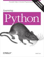
Let’s look at an example of nesting. The following interaction defines a tree of nested compound sequence objects, shown in Figure 9-1. To access its components, you may include as many index operations as required. Python evaluates the indexes from left to right, and fetches a reference to a more deeply nested object at each step. Figure 9-1 may be a pathologically complicated data structure, but it illustrates the syntax used to access nested objects in general:
L = ['abc', [(1, 2), ([3], 4)], 5]>>>L[1][(1, 2), ([3], 4)] >>>L[1][1]([3], 4) >>>L[1][1][0][3] >>>L[1][1][0][0]3
![A nested object tree with the offsets of its components, created by running the literal expression ['abc', [(1, 2), ([3], 4)], 5]. Syntactically nested objects are internally represented as references (i.e., pointers) to separate pieces of memory.](http://imgdetail.ebookreading.net/software_development/33/9780596513986/9780596513986__learning-python-3rd__9780596513986__httpatomoreillycomsourceoreillyimages15840.png)
References Versus Copies
Chapter 6 mentioned that assignments always store references to objects, not copies of those objects. In practice, this is usually what you want. Because assignments can generate multiple references to the same object, though, it’s important to be aware that changing a mutable object in-place may affect other references to the same object elsewhere in your program. If you don’t want such behavior, you’ll need to tell Python to copy the object explicitly.
We studied this phenomenon in Chapter 6, but it can become more acute
when larger objects come into play. For instance, the following example
creates a list assigned to X, and
another list assigned to L that embeds
a reference back to list X. It also
creates a dictionary D that contains
another reference back to list X:
X = [1, 2, 3]>>>L = ['a', X, 'b']# Embed references to X's object >>>D = {'x':X, 'y':2}
At this point, there are three references to the first list created:
from the name X, from inside the list
assigned to L, and from inside the
dictionary assigned to D. The situation
is illustrated in Figure 9-2.
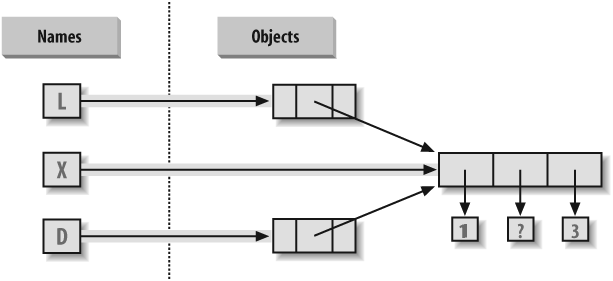
Because lists are mutable, changing the shared list object from any of the three references also changes what the other two reference:
X[1] = 'surprise'# Changes all three references! >>>L['a', [1, 'surprise', 3], 'b'] >>>D{'x': [1, 'surprise', 3], 'y': 2}
References are a higher-level analog of pointers in other languages. Although you can’t grab hold of the reference itself, it’s possible to store the same reference in more than one place (variables, lists, and so on). This is a feature—you can pass a large object around a program without generating expensive copies of it along the way. If you really do want copies, however, you can request them:
Slice expressions with empty limits (
L[:]) copy sequences.The dictionary
copymethod (D.copy( )) copies a dictionary.Some built-in functions, such as
list, make copies (list(L)).The
copystandard library module makes full copies.
For example, say you have a list and a dictionary, and you don’t want their values to be changed through other variables:
L = [1,2,3]>>>D = {'a':1, 'b':2}
To prevent this, simply assign copies to the other variables, not references to the same objects:
A = L[:]# Instead of A = L (or list(L)) >>>B = D.copy( )# Instead of B = D
This way, changes made from the other variables will change the copies, not the originals:
A[1] = 'Ni'>>>B['c'] = 'spam'>>> >>>L, D([1, 2, 3], {'a': 1, 'b': 2}) >>>A, B([1, 'Ni', 3], {'a': 1, 'c': 'spam', 'b': 2})
In terms of our original example, you can avoid the reference side effects by slicing the original list instead of simply naming it:
X = [1, 2, 3]>>>L = ['a', X[:], 'b']# Embed copies of X's object >>>D = {'x':X[:], 'y':2}
This changes the picture in Table 9-2—L
and D will now point to different lists
than X. The net effect is that changes
made through X will impact only
X, not L and D;
similarly, changes to L or D will not impact X.
One note on copies: empty-limit slices and the dictionary copy method still only make
top-level copies; that is, they do not copy nested
data structures, if any are present. If you need a complete, fully
independent copy of a deeply nested data structure, use the standard
copy module: include an import copy statement, and say X = copy.deepcopy(Y) to fully copy an
arbitrarily nested object Y. This call
recursively traverses objects to copy all their parts. This is the much
more rare case, though (which is why you have to say more to make it go).
References are usually what you will want; when they are not, slices and
copy methods are usually as much copying as you’ll need to do.
Comparisons, Equality, and Truth
All Python objects also respond to comparisons: tests for equality, relative magnitude, and so on. Python comparisons always inspect all parts of compound objects until a result can be determined. In fact, when nested objects are present, Python automatically traverses data structures to apply comparisons recursively from left to right, and as deeply as needed. The first difference found along the way determines the comparison result.
For instance, a comparison of list objects compares all their components automatically:
L1 = [1, ('a', 3)]# Same value, unique objects >>>L2 = [1, ('a', 3)]>>>L1 == L2, L1 is L2# Equivalent? Same object? (True, False)
Here, L1 and L2 are assigned lists that are equivalent but
distinct objects. Because of the nature of Python references (studied in
Chapter 6), there are two ways to
test for equality:
The
==operator tests value equivalence. Python performs an equivalence test, comparing all nested objects recursively.The
isoperator tests object identity. Python tests whether the two are really the same object (i.e., live at the same address in memory).
In the preceding example, L1 and
L2 pass the == test (they have equivalent values because all
their components are equivalent), but fail the is check (they reference two different objects,
and hence two different pieces of memory). Notice what happens for short
strings, though:
S1 = 'spam'>>>S2 = 'spam'>>>S1 == S2, S1 is S2(True, True)
Here, we should again have two distinct objects that happen to have
the same value: == should be true, and
is should be false. But because Python
internally caches and reuses short strings as an optimization, there
really is just a single string 'spam'
in memory, shared by S1 and S2; hence, the is identity test reports a true result. To
trigger the normal behavior, we need to use longer strings:
S1 = 'a longer string'>>>S2 = 'a longer string'>>>S1 == S2, S1 is S2(True, False)
Of course, because strings are immutable, the object caching mechanism is irrelevant to your code—string can’t be changed in-place, regardless of how many variables refer to them. If identity tests seem confusing, see Chapter 6 for a refresher on object reference concepts.
As a rule of thumb, the ==
operator is what you will want to use for almost all equality checks;
is is reserved for highly specialized
roles. We’ll see cases where these operators are put to use later in the
book.
Relative magnitude comparisons are also applied recursively to nested data structures:
L1 = [1, ('a', 3)]>>>L2 = [1, ('a', 2)]>>>L1 < L2, L1 == L2, L1 > L2# Less, equal, greater: tuple of results (False, False, True)
Here, L1 is greater than L2 because the nested 3 is greater than 2. The result of the last line above is really a
tuple of three objects—the results of the three expressions typed (an
example of a tuple without its enclosing parentheses).
In general, Python compares types as follows:
Numbers are compared by relative magnitude.
Strings are compared lexicographically, character by character (
"abc" < "ac").Lists and tuples are compared by comparing each component from left to right.
Dictionaries are compared as though comparing sorted (key, value) lists.
In general, comparisons of structured objects proceed as though you had written the objects as literals and compared all their parts one at a time from left to right. In later chapters, we’ll see other object types that can change the way they get compared.
The Meaning of True and False in Python
Notice that the three values in the tuple returned in the last
example of the prior section represent true and false values. They print
as the words True and False, but now that we’re using logical tests
like this one in earnest, I should be a bit more formal about what these
names really mean.
In Python, as in most programming languages, an integer 0 represents false, and an integer 1 represents true. In addition, though, Python recognizes any empty data structure as false, and any nonempty data structure as true. More generally, the notions of true and false are intrinsic properties of every object in Python—each object is either true or false, as follows:
Numbers are true if nonzero.
Other objects are true if nonempty.
Table 9-4 gives examples of true and false objects in Python.
|
Object |
Value |
|
|
|
|
|
|
|
|
|
|
|
|
|
|
|
|
|
|
|
|
|
Python also provides a special object called None (the last item in Table 9-4), which is always considered to
be false. None was introduced in
Chapter 4; it is the only value
of a special data type in Python, and typically serves as an empty
placeholder, much like a NULL pointer
in C.
For example, recall that for lists you cannot assign to an offset
unless that offset already exists (the list does not magically grow if
you make an out-of-bounds assignment). To preallocate a 100-item list
such that you can add to any of the 100 offsets, you can fill one with
None objects:
L = [None] * 100>>> >>>L[None, None, None, None, None, None, None, ... ]
The Python Boolean type bool
(introduced in Chapter 5) simply augments the notion of
true and false in Python. You may have noticed that the results of tests
in this chapter display as the words True and False. As we learned in Chapter 5, these are just customized versions of the integers
1 and 0. Because of the way this new type is implemented, this is really
just a minor extension to the notions of true and false already
described, designed to make truth values more explicit. When used
explicitly in truth tests, the words True and False evaluate to true and false because they
truly are just specialized versions of the integers 1 and 0. Results of
tests also print as the words True
and False, instead of 1 and 0.
You are not required to use only Boolean types in logical
statements such as if; all objects
are still inherently true or false, and all the Boolean concepts
mentioned in this chapter still work as described if you use other
types. We’ll explore Booleans further when we study logical statements
in Chapter 12.
Python’s Type Hierarchies
Figure 9-3 summarizes all the built-in object types available in Python and their relationships. We’ve looked at the most prominent of these; most of the other kinds of objects in Figure 9-3 correspond to program units (e.g., functions and modules), or exposed interpreter internals (e.g., stack frames and compiled code).
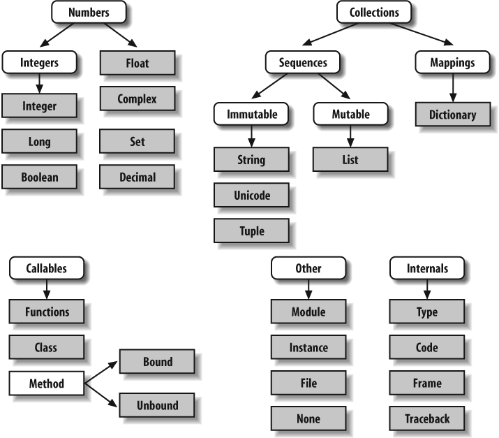
The main point to notice here is that everything is an object type in a Python system, and may be processed by your Python programs. For instance, you can pass a class to a function, assign it to a variable, stuff it in a list or dictionary, and so on.
In fact, even types themselves are an object type in Python: a call
to the built-in function type(X)
returns the type object of object X.
Type objects can be used for manual type comparisons in Python if statements. However, for reasons introduced
in Chapter 4, manual type testing
is usually not the right thing to do in Python.
One note on type names: as of Python 2.2, each core type has a new
built-in name added to support type customization through object-oriented
subclassing: dict, list, str,
tuple, int, long,
float, complex, unicode, type, and file (file is
a synonym for open). Calls to these
names are really object constructor calls, not simply conversion
functions, though you can treat them as simple functions for basic
usage.
The types standard library module
also provides additional type names (now largely synonyms for the built-in
type names), and it is possible to do type tests with the isinstance function. For example, in Python 2.2
and later, all of the following type tests are true:
Because types can be subclassed in Python today, the isinstance technique is generally recommended.
See Chapter 26 for more on subclassing
built-in types in Python 2.2 and later.
Other Types in Python
Besides the core objects studied in this part of the book, a typical Python installation has dozens of other object types available as linked-in C extensions or Python classes—regular expression objects, DBM files, GUI widgets, network sockets, and so on.
The main difference between these extra tools and the built-in types
we’ve seen so far is that the built-ins provide special language creation
syntax for their objects (e.g., 4 for
an integer, [1,2] for a list, and the
open function for files). Other tools
are generally made available in standard library modules that you must
first import to use. For instance, to make a regular expression object,
you import re and call re.compile( ). See Python’s library reference
for a comprehensive guide to all the tools available to Python
programs.
Built-in Type Gotchas
That’s the end of our look at core data types. We’ll wrap up this part of the book with a discussion of common problems that seem to bite new users (and the occasional expert) along with their solutions. Some of this is a review of ideas we’ve already covered, but these issues are important enough to warn about again here.
Assignment Creates References, Not Copies
Because this is such a central concept, I’ll mention it again: you
need to understand what’s going on with shared references in your
program. For instance, in the following example, the list object
assigned to the name L is referenced
from L and from inside the list
assigned to the name M. Changing
L in-place changes what M references, too:
L = [1, 2, 3]>>>M = ['X', L, 'Y']# Embed a reference to L >>>M['X', [1, 2, 3], 'Y'] >>>L[1] = 0# Changes M too >>>M['X', [1, 0, 3], 'Y']
This effect usually becomes important only in larger programs, and shared references are often exactly what you want. If they’re not, you can avoid sharing objects by copying them explicitly. For lists, you can always make a top-level copy by using an empty-limits slice:
L = [1, 2, 3]>>>M = ['X', L[:], 'Y']# Embed a copy of L >>>L[1] = 0# Changes only L, not M >>>L[1, 0, 3] >>>M['X', [1, 2, 3], 'Y']
Remember, slice limits default to 0, and the length of the sequence being sliced; if both are omitted, the slice extracts every item in the sequence, and so makes a top-level copy (a new, unshared object).
Repetition Adds One Level Deep
Sequence repetition is like adding a sequence to itself a number
of times. That’s true, but when mutable sequences are nested, the effect
might not always be what you expect. For instance, in the following
example X is assigned to L repeated four times, whereas Y is assigned to a list
containing L
repeated four times:
L = [4, 5, 6]>>>X = L * 4# Like [4, 5, 6] + [4, 5, 6] + ... >>>Y = [L] * 4# [L] + [L] + ... = [L, L,...] >>>X[4, 5, 6, 4, 5, 6, 4, 5, 6, 4, 5, 6] >>>Y[[4, 5, 6], [4, 5, 6], [4, 5, 6], [4, 5, 6]]
Because L was nested in the
second repetition, Y winds up
embedding references back to the original list assigned to L, and so is open to the same sorts of side
effects noted in the last section:
L[1] = 0# Impacts Y but not X >>>X[4, 5, 6, 4, 5, 6, 4, 5, 6, 4, 5, 6] >>>Y[[4, 0, 6], [4, 0, 6], [4, 0, 6], [4, 0, 6]]
The same solutions to this problem apply here as in the previous section, as this is really just another way to create the shared mutable object reference case. If you remember that repetition, concatenation, and slicing copy only the top level of their operand objects, these sorts of cases make much more sense.
Beware of Cyclic Data Structures
We actually encountered this concept in a prior exercise: if a
collection object contains a reference to itself, it’s called a
cyclic object. Python prints a [...] whenever it detects a cycle in the
object, rather than getting stuck in an infinite loop:
L = ['grail']# Append reference to same object >>>L.append(L)# Generates cycle in object: [...] >>>L['grail', [...]]
Besides understanding that the three dots in square brackets represent a cycle in the object, this case is worth knowing about because it can lead to gotchas—cyclic structures may cause code of your own to fall into unexpected loops if you don’t anticipate them. For instance, some programs keep a list or dictionary of items already visited, and check it to determine whether they’re in a cycle. See the solutions to "Part I Exercises" in Chapter 3 for more on this problem, and check out the reloadall.py program at the end of Chapter 21 for a solution.
Don’t use a cyclic reference unless you need to. There are good reasons to create cycles, but unless you have code that knows how to handle them, you probably won’t want to make your objects reference themselves very often in practice.
Immutable Types Can’t Be Changed In-Place
Finally, you can’t change an immutable object in-place. Instead, construct a new object with slicing, concatenation, and so on, and assign it back to the original reference, if needed:
That might seem like extra coding work, but the upside is that the previous gotchas can’t happen when you’re using immutable objects such as tuples and strings; because they can’t be changed in-place, they are not open to the sorts of side effects that lists are.
Chapter Summary
This chapter explored the last two major core object types—the tuple
and the file. We learned that tuples support all the usual sequence
operations, but they have no methods, and do not allow any in-place
changes because they are immutable. We also learned that files are
returned by the built-in open function
and provide methods for reading and writing data. We explored how to
translate Python objects to and from strings for storing in files, and we
looked at the pickle and struct modules for advanced roles (object
serialization and binary data). Finally, we wrapped up by reviewing some
properties common to all object types (e.g., shared references) and went
through a list of common mistakes (“gotchas”) in the object type
domain.
In the next part, we’ll shift gears, turning to the topic of statement syntax in Python—we’ll explore all of Python’s basic procedural statements in the chapters that follow. The next chapter kicks off that part of the book with an introduction to Python’s general syntax model, which is applicable to all statement types. Before moving on, though, take the chapter quiz, and then work through the end-of-part lab exercises to review type concepts. Statements largely just create and process objects, so make sure you’ve mastered this domain by working through all the exercises before reading on.
BRAIN BUILDER
BRAIN BUILDER
Part II Exercises
This session asks you to get your feet wet with built-in object fundamentals. As before, a few new ideas may pop up along the way, so be sure to flip to the answers in Appendix B when you’re done (and even when you’re not). If you have limited time, I suggest starting with exercises 10 and 11 (the most practical of the bunch), and then working from first to last as time allows. This is all fundamental material, though, so try to do as many of these as you can.
The basics. Experiment interactively with the common type operations found in the tables in Part II. To get started, bring up the Python interactive interpreter, type each of the following expressions, and try to explain what’s happening in each case:
    2 ** 16
    2 / 5, 2 / 5.0

    "spam" + "eggs"
    S = "ham"
    "eggs " + S
    S * 5
    S[:0]
    "green %s and %s" % ("eggs", S)

    ('x',)[0]
    ('x', 'y')[1]

    L = [1,2,3] + [4,5,6]
    L, L[:], L[:0], L[−2], L[−2:]
    ([1,2,3] + [4,5,6])[2:4]
    [L[2], L[3]]
    L.reverse(  ); L
    L.sort(  ); L
    L.index(4)

    {'a':1, 'b':2}['b']
    D = {'x':1, 'y':2, 'z':3}
    D['w'] = 0
    D['x'] + D['w']
    D[(1,2,3)] = 4
    D.keys(  ), D.values(  ), D.has_key((1,2,3))

    [[]], ["",[],(  ),{},None]
Indexing and slicing. At the interactive prompt, define a list named
Lthat contains four strings or numbers (e.g.,L=[0,1,2,3]). Then, experiment with some boundary cases:What happens when you try to index out of bounds (e.g.,
L[4])?What about slicing out of bounds (e.g.,
L[−1000:100])?Finally, how does Python handle it if you try to extract a sequence in reverse, with the lower bound greater than the higher bound (e.g.,
L[3:1])? Hint: try assigning to this slice (L[3:1]=['?']), and see where the value is put. Do you think this may be the same phenomenon you saw when slicing out of bounds?
Indexing, slicing, and
del. Define another listLwith four items, and assign an empty list to one of its offsets (e.g.,L[2]=[]). What happens? Then, assign an empty list to a slice (L[2:3]=[]). What happens now? Recall that slice assignment deletes the slice, and inserts the new value where it used to be.The
delstatement deletes offsets, keys, attributes, and names. Use it on your list to delete an item (e.g.,del L[0]). What happens if you delete an entire slice (del L[1:])? What happens when you assign a nonsequence to a slice (L[1:2]=1)?Tuple assignment. Type the following lines:
>>> X = 'spam'>>>Y = 'eggs'>>>X, Y = Y, XWhat do you think is happening to
XandYwhen you type this sequence?Dictionary keys. Consider the following code fragments:
>>> D = {}>>>D[1] = 'a'>>>D[2] = 'b'You’ve learned that dictionaries aren’t accessed by offsets, so what’s going on here? Does the following shed any light on the subject? (Hint: strings, integers, and tuples share which type category?)
>>> D[(1, 2, 3)] = 'c'>>>D{1: 'a', 2: 'b', (1, 2, 3): 'c'}Dictionary indexing. Create a dictionary named
Dwith three entries, for keys'a','b', and'c'. What happens if you try to index a nonexistent key (D['d'])? What does Python do if you try to assign to a nonexistent key'd'(e.g.,D['d']='spam')? How does this compare to out-of-bounds assignments and references for lists? Does this sound like the rule for variable names?Generic operations. Run interactive tests to answer the following questions:
What happens when you try to use the
+operator on different/mixed types (e.g., string+list, list+tuple)?Does
+work when one of the operands is a dictionary?Does the
appendmethod work for both lists and strings? How about using thekeysmethod on lists? (Hint: What doesappendassume about its subject object?)Finally, what type of object do you get back when you slice or concatenate two lists or two strings?
String indexing. Define a string
Sof four characters:S = "spam". Then type the following expression:S[0][0][0][0][0]. Any clue as to what’s happening this time? (Hint: recall that a string is a collection of characters, but Python characters are one-character strings.) Does this indexing expression still work if you apply it to a list such as['s', 'p', 'a', 'm']? Why?Immutable types. Define a string
Sof four characters again:S = "spam". Write an assignment that changes the string to"slam", using only slicing and concatenation. Could you perform the same operation using just indexing and concatenation? How about index assignment?Nesting. Write a data structure that represents your personal information: name (first, middle, last), age, job, address, email address, and phone number. You may build the data structure with any combination of built-in object types you like (lists, tuples, dictionaries, strings, numbers). Then, access the individual components of your data structures by indexing. Do some structures make more sense than others for this object?
Files. Write a script that creates a new output file called myfile.txt, and writes the string
"Hello file
          world!"
into it. Then, write another script that opens myfile.txt and reads and prints its contents. Run your two scripts from the system command line. Does the new file show up in the directory where you ran your scripts? What if you add a different directory path to the filename passed toopen? Note: filewritemethods do not add newline characters to your strings; add an explicitThe
dirfunction revisited. Try typing the following expressions at the interactive prompt. Starting with version 1.5, thedirfunction has been generalized to list all attributes of any Python object you’re likely to be interested in. If you’re using an earlier version than 1.5, the_ _methods_ _scheme has the same effect. If you’re using Python 2.2,diris probably the only of these that will work.
    []._  _methods_  _         # 1.4 or 1.5
    dir([])                    # 1.5 and later

    {}._  _methods_  _         # Dictionary
    dir({})