There are two ways of accessing columns: you can get a single column at a time by accessing them as if they were a DataShape attribute:

traffic.Year.head(2)

The preceding script produces the following output:

You can also use indexing that allows the selection of more than one column at a time:

(traffic[['Location', 'Year', 'Accident', 'Fatal', 'Alcohol']]
    .head(2))

This generates the following output:

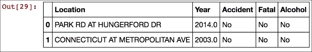
The preceding syntax would be the same for pandas DataFrames. For those of you unfamiliar with Python and pandas API, please note three things here:

The beauty of Blaze comes from the fact that it can operate symbolically. What this means is that you can specify transformations, filters, or other operations on your data and store them as object(s). You can then feed such object with almost any form of data conforming to the original schema, and Blaze will return the transformed data.

For example, let's select all the traffic violations that occurred in 2013, and return only the 'Arrest_Type', 'Color', and 'Charge` columns. First, if we could not reflect the schema from an already existing object, we would have to specify the schema manually. To do this, we will use the .symbol(...) method to achieve that; the first argument to the method specifies a symbolic name of the transformation (we prefer keeping it the same as the name of the object, but it can be anything), and the second argument is a long string that specifies the schema in a <column_name>: <column_type> fashion, separated by commas:

schema_example = bl.symbol('schema_exampl', 
                           '{id: int, name: string}')

Now, you could use the schema_example object and specify some transformations. However, since we already have an existing traffic dataset, we can reuse the schema by using traffic.dshape and specifying our transformations:

traffic_s = bl.symbol('traffic', traffic.dshape)
traffic_2013 = traffic_s[traffic_s['Stop_year'] == 2013][
    ['Stop_year', 'Arrest_Type','Color', 'Charge']
]

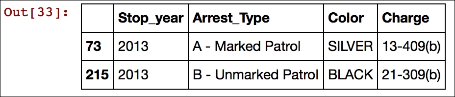
To present how this works, let's read the original dataset into pandas' DataFrame:

traffic_pd = pd.read_csv('../Data/TrafficViolations.csv')

Once read, we pass the dataset directly to the traffic_2013 object and perform the computation using the .compute(...) method of Blaze; the first argument to the method specifies the transformation object (ours is traffic_2013) and the second parameter is the data that the transformations are to be performed on:

bl.compute(traffic_2013, traffic_pd).head(2)

Here is the output of the preceding snippet:

You can also pass a list of lists or a list of NumPy arrays. Here, we use the .values attribute of the DataFrame to access the underlying list of NumPy arrays that form the DataFrame:

bl.compute(traffic_2013, traffic_pd.values)[0:2]

This code will produce precisely what we would expect:

Blaze allows for easy mathematical operations to be done on numeric columns. All the traffic violations cited in the dataset occurred between 2013 and 2016. You can check that by getting all the distinct values for the Stop_year column using the .distinct() method. The .sort() method sorts the results in an ascending order:

traffic['Stop_year'].distinct().sort()

The preceding code produces the following output table:

An equivalent syntax for pandas would be as follows:

traffic['Stop_year'].unique().sort()

For SQL, use the following code:

SELECT DISTINCT Stop_year
FROM traffic

You can also make some mathematical transformations/arithmetic to the columns. Since all the traffic violations occurred after year 2000, we can subtract 2000 from the Stop_year column without losing any accuracy:

traffic['Stop_year'].head(2) - 2000

Here is what you should get in return:

The same could be attained from pandas DataFrame with an identical syntax (assuming traffic was of pandas DataFrame type). For SQL, the equivalent would be:

SELECT Stop_year - 2000 AS Stop_year
FROM traffic

However, if you want to do some more complex mathematical operations (for example, log or pow) then you first need to use the one provided by Blaze (that, in the background, will translate your command to a suitable method from NumPy, math, or pandas).

For example, if you wanted to log-transform the Stop_year you need to use this code:

bl.log(traffic['Stop_year']).head(2)

This will produce the following output:

Some reduction methods are also available, such as .mean() (that calculates the average), .std (that calculates standard deviation), or .max() (that returns the maximum from the list). Executing the following code:

traffic['Stop_year'].max()

It will return the following output:

If you had a pandas DataFrame you can use the same syntax, whereas for SQL the same could be done with the following code:

SELECT MAX(Stop_year) AS Stop_year_max
FROM traffic

It is also quite easy to add more columns to your dataset. Say, you wanted to calculate the age of the car (in years) at the time when the violation occurred. First, you would take the Stop_year and subtract the Year of manufacture.

In the following code snippet, the first argument to the .transform(...) method is the DataShape, the transformation is to be performed on, and the other(s) would be a list of transformations.

traffic = bl.transform(traffic,
             Age_of_car = traffic.Stop_year - traffic.Year)
traffic.head(2)

The above code produces the following table:

An equivalent operation in pandas could be attained through the following code:

traffic['Age_of_car'] = traffic.apply(
    lambda row: row.Stop_year - row.Year,
    axis = 1
)

For SQL you can use the following code:

SELECT *
    , Stop_year - Year AS Age_of_car
FROM traffic

If you wanted to calculate the average age of the car involved in a fatal traffic violation and count the number of occurrences, you can perform a group by operation using the .by(...) operation:

bl.by(traffic['Fatal'], 
      Fatal_AvgAge=traffic.Age_of_car.mean(),
      Fatal_Count =traffic.Age_of_car.count()
)

The first argument to .by(...) specifies the column of the DataShape to perform the aggregation by, followed by a series of aggregations we want to get. In this example, we select the Age_of_car column and calculate an average and count the number of rows per each value of the 'Fatal' column.

The preceding script produces the following aggregation:

For pandas, an equivalent would be as follows:

traffic
    .groupby('Fatal')['Age_of_car']
    .agg({
        'Fatal_AvgAge': np.mean,
        'Fatal_Count':  np.count_nonzero
    })

For SQL, it would be as follows:

SELECT Fatal
    , AVG(Age_of_car)   AS Fatal_AvgAge
    , COUNT(Age_of_car) AS Fatal_Count
FROM traffic
GROUP BY Fatal

Joining two DataShapes is straightforward as well. To present how this is done, although the same result could be attained differently, we first select all the traffic violations by violation type (the violation object) and the traffic violations involving belts (the belts object):

violation = traffic[
    ['Stop_month','Stop_day','Stop_year',
     'Stop_hr','Stop_min','Stop_sec','Violation_Type']]
belts = traffic[
    ['Stop_month','Stop_day','Stop_year',
     'Stop_hr','Stop_min','Stop_sec','Belts']]

Now, we join the two objects on the six date and time columns.

The first argument to the .join(...) method is the first DataShape we want to join with, the second argument is the second DataShape, while the third argument can be either a single column or a list of columns to perform the join on:

violation_belts = bl.join(violation, belts, 
      ['Stop_month','Stop_day','Stop_year',
       'Stop_hr','Stop_min','Stop_sec'])

Once we have the full dataset in place, let's check how many traffic violations involved belts and what sort of punishment was issued to the driver:

bl.by(violation_belts[['Violation_Type', 'Belts']],
      Violation_count=violation_belts.Belts.count()
).sort('Violation_count', ascending=False)

Here's the output of the preceding script:

The same could be achieved in pandas with the following code:

violation.merge(belts, 
    on=['Stop_month','Stop_day','Stop_year',
        'Stop_hr','Stop_min','Stop_sec']) 
    .groupby(['Violation_type','Belts']) 
    .agg({
        'Violation_count':  np.count_nonzero
    }) 
    .sort('Violation_count', ascending=False)

With SQL, you would use the following snippet:

SELECT innerQuery.*
FROM (
    SELECT a.Violation_type
        , b.Belts
        , COUNT() AS Violation_count
    FROM violation AS a
    INNER JOIN belts AS b
        ON      a.Stop_month = b.Stop_month
            AND a.Stop_day = b.Stop_day
            AND a.Stop_year = b.Stop_year
            AND a.Stop_hr = b.Stop_hr
            AND a.Stop_min = b.Stop_min
            AND a.Stop_sec = b.Stop_sec
    GROUP BY Violation_type
        , Belts
) AS innerQuery
ORDER BY Violation_count DESC