
CHAPTER 3
Discounted Cash Flow Analysis
Discounted cash flow analysis (“DCF analysis” or the “DCF”) is a fundamental valuation methodology broadly used by investment bankers, corporate officers, university professors, investors, and other finance professionals. It is premised on the principle that the value of a company, division, business, or collection of assets (“target”) can be derived from the present value of its projected free cash flow (FCF). A company's projected FCF is derived from a variety of assumptions and judgments about its expected financial performance, including sales growth rates, profit margins, capital expenditures, and net working capital (NWC) requirements. The DCF has a wide range of applications, including valuation for various M&A situations, IPOs, restructurings, and investment decisions.
The valuation implied for a target by a DCF is also known as its intrinsic value, as opposed to its market value, which is the value ascribed by the market at a given point in time. As a result, when performing a comprehensive valuation, a DCF serves as an important alternative to market-based valuation techniques such as comparable companies and precedent transactions, which can be distorted by a number of factors, including market aberrations (e.g., the post-subprime credit crunch). As such, a DCF plays an important role as a check on the prevailing market valuation for a publicly traded company. A DCF is also valuable when there are limited (or no) pure play, peer companies or comparable acquisitions.
In a DCF, a company's FCF is typically projected for a period of five years. The projection period, however, may be longer depending on the company's sector, stage of development, and the underlying predictability of its financial performance. Given the inherent difficulties in accurately projecting a company's financial performance over an extended period of time (and through various business and economic cycles), a terminal value is used to capture the remaining value of the target beyond the projection period (i.e., its “going concern” value).
The projected FCF and terminal value are discounted to the present at the target's weighted average cost of capital (WACC), which is a discount rate commensurate with its business and financial risks. The present value of the FCF and terminal value are summed to determine an enterprise value, which serves as the basis for the DCF valuation. The WACC and terminal value assumptions typically have a substantial impact on the output, with even slight variations producing meaningful differences in valuation. As a result, a DCF output is viewed in terms of a valuation range based on a range of key input assumptions, rather than as a single value. The impact of these assumptions on valuation is tested using sensitivity analysis.
The assumptions driving a DCF are both its primary strength and weakness versus market-based valuation techniques. On the positive side, the use of defensible assumptions regarding financial projections, WACC, and terminal value helps shield the target's valuation from market distortions that occur periodically. In addition, a DCF provides the flexibility to analyze the target's valuation under different scenarios by changing the underlying inputs and examining the resulting impact. On the negative side, a DCF is only as strong as its assumptions. Hence, assumptions that fail to adequately capture the realistic set of opportunities and risks facing the target will also fail to produce a meaningful valuation.
This chapter walks through a step-by-step construction of a DCF, or its science (see Exhibit 3.1). At the same time, it provides the tools to master the art of the DCF, namely the ability to craft a logical set of assumptions based on an in-depth analysis of the target and its key performance drivers. Once this framework is established, we perform an illustrative DCF analysis for our target company, ValueCo.

EXHIBIT 3.1 Discounted Cash Flow Analysis Steps
Summary of Discounted Cash Flow Analysis Steps
- Step I. Study the Target and Determine Key Performance Drivers. The first step in performing a DCF, as with any valuation exercise, is to study and learn as much as possible about the target and its sector. Shortcuts in this critical area of due diligence may lead to misguided assumptions and valuation distortions later on. This exercise involves determining the key drivers of financial performance (in particular sales growth, profitability, and FCF generation), which enables the banker to craft (or support) a defensible set of projections for the target. Step I is invariably easier when valuing a public company as opposed to a private company due to the availability of information from sources such as SEC filings (e.g., 10-Ks, 10-Qs, and 8-Ks), equity research reports, earnings call transcripts, and investor presentations.
For private, non-filing companies, the banker often relies upon company management to provide materials containing basic business and financial information. In an organized M&A sale process, this information is typically provided in the form of a CIM (see Chapter 6). In the absence of this information, alternative sources (e.g., company websites, trade journals, and news articles, as well as SEC filings and research reports for public competitors, customers, and suppliers) must be used to learn basic company information and form the basis for developing the assumptions to drive financial projections.
- Step II. Project Free Cash Flow. The projection of the target's unlevered FCF forms the core of a DCF. Unlevered FCF, which we simply refer to as FCF in this chapter, is the cash generated by a company after paying all cash operating expenses and taxes, as well as the funding of capex and working capital, but prior to the payment of any interest expense.1 The target's projected FCF is driven by assumptions underlying its future financial performance, including sales growth rates, profit margins, capex, and working capital requirements. Historical performance, combined with third party and/or management guidance, helps in developing these assumptions. The use of realistic FCF projections is critical as it has the greatest effect on valuation in a DCF.
In a DCF, the target's FCF is typically projected for a period of five years, but this period may vary depending on the target's sector, stage of development, and the predictability of its FCF. However, five years is typically sufficient for spanning at least one business/economic cycle and allowing for the successful realization of in-process or planned initiatives. The goal is to project FCF to a point in the future when the target's financial performance is deemed to have reached a “steady state” that can serve as the basis for a terminal value calculation (see Step IV).
- Step III. Calculate Weighted Average Cost of Capital. In a DCF, WACC is the rate used to discount the target's projected FCF and terminal value to the present. It is designed to fairly reflect the target's business and financial risks. As its name connotes, WACC represents the “weighted average” of the required return on the invested capital (customarily debt and equity) in a given company. It is also commonly referred to as a company's discount rate or cost of capital. As debt and equity components generally have significantly different risk profiles and tax ramifications, WACC is dependent on capital structure.
- Step IV. Determine Terminal Value. The DCF approach to valuation is based on determining the present value of future FCF produced by the target. Given the challenges of projecting the target's FCF indefinitely, a terminal value is used to quantify the remaining value of the target after the projection period. The terminal value typically accounts for a substantial portion of the target's value in a DCF. Therefore, it is important that the target's financial data in the final year of the projection period (“terminal year”) represents a steady state or normalized level of financial performance, as opposed to a cyclical high or low.
There are two widely accepted methods used to calculate a company's terminal value—the exit multiple method (EMM) and the perpetuity growth method (PGM). The EMM calculates the remaining value of the target after the projection period on the basis of a multiple of the target's terminal year EBITDA (or EBIT). The PGM calculates terminal value by treating the target's terminal year FCF as a perpetuity growing at an assumed rate.
- Step V. Calculate Present Value and Determine Valuation. The target's projected FCF and terminal value are discounted to the present and summed to calculate its enterprise value. Implied equity value and share price (if relevant) can then be derived from the calculated enterprise value. The present value calculation is performed by multiplying the FCF for each year in the projection period, as well as the terminal value, by its respective discount factor. The discount factor represents the present value of one dollar received at a given future date assuming a given discount rate.2
As a DCF incorporates numerous assumptions about key performance drivers, WACC, and terminal value, it is used to produce a valuation range rather than a single value. The exercise of driving a valuation range by varying key inputs is called sensitivity analysis. Core DCF valuation drivers such as WACC, exit multiple or perpetuity growth rate, sales growth rates, and margins are the most commonly sensitized inputs. Once determined, the valuation range implied by the DCF should be compared to those derived from other methodologies such as comparable companies, precedent transactions, and LBO analysis (if applicable) as a sanity check.
Once the step-by-step approach summarized above is complete, the final DCF output page should look similar to the one shown in Exhibit 3.2.

EXHIBIT 3.2 DCF Analysis Output Page
STEP I. STUDY THE TARGET AND DETERMINE KEY PERFORMANCE DRIVERS
Study the Target
The first step in performing a DCF, as with any valuation exercise, is to study and learn as much as possible about the target and its sector. A thorough understanding of the target's business model, financial profile, value proposition for customers, end markets, competitors, and key risks is essential for developing a framework for valuation. The banker needs to be able to craft (or support) a realistic set of financial projections, as well as WACC and terminal value assumptions, for the target. Performing this task is invariably easier when valuing a public company as opposed to a private company due to the availability of information.
For a public company,3 a careful reading of its recent SEC filings (e.g., 10-Ks, 10-Qs, and 8-Ks), earnings call transcripts, and investor presentations provides a solid introduction to its business and financial characteristics. To determine key performance drivers, the MD&A sections of the most recent 10-K and 10-Q are an important source of information as they provide a synopsis of the company's financial and operational performance during the prior reporting periods, as well as management's outlook for the company. Equity research reports add additional color and perspective while typically providing financial performance estimates for the future two- or three-year period.
For private, non-filing companies or smaller divisions of public companies (for which segmented information is not provided), company management is often relied upon to provide materials containing basic business and financial information. In an organized M&A sale process, this information is typically provided in the form of a CIM. In the absence of this information, alternative sources must be used, such as company websites, trade journals, and news articles, as well as SEC filings and research reports for public competitors, customers, and suppliers. For those private companies that were once public filers, or operated as a subsidiary of a public filer, it can be informative to read through old filings or research reports.
Determine Key Performance Drivers
The next level of analysis involves determining the key drivers of a company's performance (particularly sales growth, profitability, and FCF generation) with the goal of crafting (or supporting) a defensible set of FCF projections. These drivers can be both internal (such as opening new facilities/stores, developing new products, securing new customer contracts, and improving operational and/or working capital efficiency) as well as external (such as acquisitions, end market trends, consumer buying patterns, macroeconomic factors, or even legislative/regulatory changes).
A given company's growth profile can vary significantly from that of its peers within the sector with certain business models and management teams more focused on, or capable of, expansion. Profitability may also vary for companies within a given sector depending on a multitude of factors including management, brand, customer base, operational focus, product mix, sales/marketing strategy, scale, and technology. Similarly, in terms of FCF generation, there are often meaningful differences among peers in terms of capex (e.g., expansion projects or owned versus leased machinery) and working capital efficiency, for example.
STEP II. PROJECT FREE CASH FLOW
After studying the target and determining key performance drivers, the banker is prepared to project its FCF. As previously discussed, FCF is the cash generated by a company after paying all cash operating expenses and associated taxes, as well as the funding of capex and working capital, but prior to the payment of any interest expense (see Exhibit 3.3). FCF is independent of capital structure as it represents the cash available to all capital providers (both debt and equity holders).

EXHIBIT 3.3 Free Cash Flow Calculation
Considerations for Projecting Free Cash Flow
Historical Performance
Historical performance provides valuable insight for developing defensible assumptions to project FCF. Past growth rates, profit margins, and other ratios are usually a reliable indicator of future performance, especially for mature companies in non-cyclical sectors. While it is informative to review historical data from as long a time horizon as possible, typically the prior three-year period (if available) serves as a good proxy for projecting future financial performance.
Therefore, as the output in Exhibit 3.2 demonstrates, the DCF customarily begins by laying out the target's historical financial data for the prior three-year period. This historical financial data is sourced from the target's financial statements with adjustments made for non-recurring items and recent events, as appropriate, to provide a normalized basis for projecting financial performance. Reported and adjusted historical financials, as well as consensus estimates are available via Bloomberg Financial Analysis (FA<GO>, see Appendix 3.1).
Projection Period Length
Typically, the banker projects the target's FCF for a period of five years depending on its sector, stage of development, and the predictability of its financial performance. As discussed in Step IV, it is critical to project FCF to a point in the future where the target's financial performance reaches a steady state or normalized level. For mature companies in established industries, five years is often sufficient for allowing a company to reach its steady state. A five-year projection period typically spans at least one business cycle and allows sufficient time for the successful realization of in-process or planned initiatives.
In situations where the target is in the early stages of rapid growth, however, it may be more appropriate to build a longer-term projection model (e.g., ten years or more) to allow the target to reach a steady state level of cash flow. In addition, a longer projection period is often used for businesses in sectors with long-term, contracted revenue streams such as natural resources, satellite communications, or utilities.
Alternative Cases
Whether advising on the buy-side or sell-side of an organized M&A sale process, the banker typically receives five years of financial projections for the target, which is usually labeled “Management Case.” At the same time, the banker must develop a sufficient degree of comfort to support and defend these assumptions. Often, the banker makes adjustments to management's projections that incorporate assumptions deemed more probable, known as the “Base Case,” while also crafting upside and downside cases.
The development of alternative cases requires a sound understanding of company-specific performance drivers as well as sector trends. The banker enters the various assumptions that drive these cases into assumptions pages (see Chapter 5, Exhibits 5.52 and 5.53), which feed into the DCF output page (see Exhibit 3.2). A “switch” or “toggle” function in the model allows the banker to move between cases without having to re-input the financial data by entering a number or letter (that corresponds to a particular set of assumptions) into a single cell.
Projecting Financial Performance without Management Guidance
In some instances, a DCF is performed without the benefit of receiving an initial set of projections. For publicly traded companies, consensus research estimates for financial statistics such as sales, EBITDA, and EBIT (which are generally provided for a future two- or three-year period) are typically used to form the basis for developing a set of projections. Individual equity research reports may provide additional financial detail, including (in some instances) a full scale two-year (or more) projection model. For private companies, a robust DCF often depends on receiving financial projections from company management. In practice, however, this is not always possible. Therefore, the banker must develop the skill set necessary to reasonably forecast financial performance in the absence of management projections. In these instances, the banker typically relies upon historical financial performance, sector trends, and consensus estimates for public comparable companies to drive defensible projections. The remainder of this section provides a detailed discussion of the major components of FCF, as well as practical approaches for projecting FCF without the benefit of readily available projections or management guidance.
Projection of Sales, EBITDA, and EBIT
Sales Projections
For public companies, the banker often sources top line projections for the first two or three years of the projection period from consensus estimates. Similarly, for private companies, consensus estimates for peer companies can be used as a proxy for expected sales growth rates, provided the trend line is consistent with historical performance and sector outlook.
As equity research normally does not provide estimates beyond a future two- or three-year period (excluding initiating coverage reports), the banker must derive growth rates in the outer years from alternative sources. Without the benefit of management guidance, this typically involves more art than science. Often, industry reports and consulting studies provide estimates on longer-term sector trends and growth rates. In the absence of reliable guidance, the banker typically steps down the growth rates incrementally in the outer years of the projection period to arrive at a reasonable long-term growth rate by the terminal year (e.g., 2% to 4%).
For a highly cyclical business such as a steel or lumber company, however, sales levels need to track the movements of the underlying commodity cycle. Consequently, sales trends are typically more volatile and may incorporate dramatic peak-to-trough swings depending on the company's point in the cycle at the start of the projection period. Regardless of where in the cycle the projection period begins, it is crucial that the terminal year financial performance represents a normalized level as opposed to a cyclical high or low. Otherwise, the company's terminal value, which usually comprises a substantial portion of the overall value in a DCF, will be skewed toward an unrepresentative level. Therefore, in a DCF for a cyclical company, top line projections might peak (or trough) in the early years of the projection period and then decline (or increase) precipitously before returning to a normalized level by the terminal year.
Once the top line projections are established, it is essential to give them a sanity check versus the target's historical growth rates as well as peer estimates and sector/market outlook. Even when sourcing information from consensus estimates, each year's growth assumptions need to be justifiable, whether on the basis of market share gains/declines, end market trends, product mix changes, demand shifts, pricing increases, or acquisitions, for example. Furthermore, the banker must ensure that sales projections are consistent with other related assumptions in the DCF, such as those for capex and working capital. For example, higher top line growth typically requires the support of higher levels of capex and working capital.
COGS and SG&A Projections
For public companies, the banker typically relies upon historical COGS4 (gross margin) and SG&A levels (as a percentage of sales) and/or sources estimates from research to drive the initial years of the projection period, if available. For the outer years of the projection period, it is common to hold gross margin and SG&A as a percentage of sales constant, although the banker may assume a slight improvement (or decline) if justified by company trends or outlook for the sector/market. Similarly, for private companies, the banker usually relies upon historical trends to drive gross profit and SG&A projections, typically holding margins constant at the prior historical year levels. At the same time, the banker may also examine research estimates for peer companies to help craft/support the assumptions and provide insight on trends.
In some cases, the DCF may be constructed on the basis of EBITDA and EBIT projections alone, thereby excluding line item detail for COGS and SG&A. This approach generally requires that NWC be driven as a percentage of sales as COGS detail for driving inventory and accounts payable is unavailable (see Exhibits 3.9, 3.10, and 3.11). However, the inclusion of COGS and SG&A detail allows the banker to drive multiple operating scenarios on the basis of gross margins and/or SG&A efficiency.
EBITDA and EBIT Projections
For public companies, EBITDA and EBIT projections for the future two- or three-year period are typically sourced from (or benchmarked against) consensus estimates, if available.5 These projections inherently capture both gross profit performance and SG&A expenses. A common approach for projecting EBITDA and EBIT for the outer years is to hold their margins constant at the level represented by the last year provided by consensus estimates (assuming the last year of estimates is representative of a steady state level). As previously discussed, however, increasing (or decreasing) levels of profitability may be modeled throughout the projection period, perhaps due to product mix changes, cyclicality, operating leverage,6 or pricing power/pressure.
For private companies, the banker looks at historical trends as well as consensus estimates for peer companies for insight on projected margins. In the absence of sufficient information to justify improving or declining margins, the banker may simply hold margins constant at the prior historical year level to establish a baseline set of projections.
Projection of Free Cash Flow
In a DCF analysis, EBIT typically serves as the springboard for calculating FCF (see Exhibit 3.4). To bridge from EBIT to FCF, several additional items need to be determined, including the marginal tax rate, D&A, capex, and changes in net working capital.

EXHIBIT 3.4 EBIT to FCF
Tax Projections
The first step in calculating FCF from EBIT is to net out estimated taxes. The result is tax-effected EBIT, also known as EBIAT or NOPAT. This calculation involves multiplying EBIT by (1 – t), where “t” is the target's marginal tax rate. A marginal tax rate of 35% to 40% is generally assumed for modeling purposes, but the company's actual tax rate (effective tax rate) in previous years can also serve as a reference point.7
Depreciation & Amortization Projections
Depreciation is a non-cash expense that approximates the reduction of the book value of a company's long-term fixed assets or property, plant, and equipment (PP&E) over an estimated useful life and reduces reported earnings. Amortization, like depreciation, is a non-cash expense that reduces the value of a company's definite life intangible assets and also reduces reported earnings.8
Some companies report D&A together as a separate line item on their income statement, but these expenses are more commonly included in COGS (especially for manufacturers of goods) and, to a lesser extent, SG&A. Regardless, D&A is explicitly disclosed in the cash flow statement as well as the notes to a company's financial statements. As D&A is a non-cash expense, it is added back to EBIAT in the calculation of FCF (see Exhibit 3.4). Hence, while D&A decreases a company's reported earnings, it does not decrease its FCF.
Depreciation
Depreciation expenses are typically scheduled over several years corresponding to the useful life of each of the company's respective asset classes. The straight-line depreciation method assumes a uniform depreciation expense over the estimated useful life of an asset. For example, an asset purchased for $100 million that is determined to have a ten-year useful life would be assumed to have an annual depreciation expense of $10 million per year for ten years. Most other depreciation methods fall under the category of accelerated depreciation, which assumes that an asset loses most of its value in the early years of its life (i.e., the asset is depreciated on an accelerated schedule allowing for greater deductions earlier on).
For DCF modeling purposes, depreciation is often projected as a percentage of sales or capex based on historical levels as it is directly related to a company's capital spending, which, in turn, tends to support top line growth. An alternative approach is to build a detailed PP&E schedule9 based on the company's existing depreciable net PP&E base and incremental capex projections. This approach involves assuming an average remaining life for current depreciable net PP&E as well as a depreciation period for new capex. While more technically sound than the “quick-and-dirty” method of projecting depreciation as a percentage of sales or capex, building a PP&E schedule generally does not yield a substantially different result.
For a DCF constructed on the basis of EBITDA and EBIT projections, depreciation (and amortization) can simply be calculated as the difference between the two. In this scenario however, the banker must ensure that the implied D&A is consistent with historical levels as well as capex projections.10 Regardless of which approach is used, the banker often makes a simplifying assumption that depreciation and capex are in line by the final year of the projection period so as to ensure that the company's PP&E base remains steady in perpetuity. Otherwise, the company's valuation would be influenced by an expanding or diminishing PP&E base, which would not be representative of a steady state business.
Amortization
Amortization differs from depreciation in that it reduces the value of definite life intangible assets as opposed to tangible assets. Definite life intangible assets include contractual rights such as non-compete clauses, copyrights, licenses, patents, trademarks, or other intellectual property, as well as information technology and customer lists, among others. These intangible assets are amortized according to a determined or useful life.11
Like depreciation, amortization can be projected as a percentage of sales or by building a detailed schedule based upon a company's existing intangible assets. However, amortization is often combined with depreciation as a single line item within a company's financial statements. Therefore, it is more common to simply model amortization with depreciation as part of one line-item (D&A).
Assuming depreciation and amortization are combined as one line item, D&A is projected in accordance with one of the approaches described under the “Depreciation” heading (e.g., as a percentage of sales or capex, through a detailed schedule, or as the difference between EBITDA and EBIT).
Capital Expenditures Projections
Capital expenditures are the funds that a company uses to purchase, improve, expand, or replace physical assets such as buildings, equipment, facilities, machinery, and other assets. Capex is an expenditure as opposed to an expense. It is capitalized on the balance sheet once the expenditure is made and then expensed over its useful life as depreciation through the company's income statement. As opposed to depreciation, capital expenditures represent actual cash outflows and, consequently, must be subtracted from EBIAT in the calculation of FCF (in the year in which the purchase is made).
Historical capex is disclosed directly on a company's cash flow statement under the investing activities section and also discussed in the MD&A section of a public company's 10-K and 10-Q. Historical levels generally serve as a reliable proxy for projecting future capex. However, capex projections may deviate from historical levels in accordance with the company's strategy, sector, or phase of operations. For example, a company in expansion mode might have elevated capex levels for some portion of the projection period, while one in harvest or cash conservation mode might limit its capex.
For public companies, future planned capex is often discussed in the MD&A of its 10-K. Research reports may also provide capex estimates for the future two- or three-year period. In the absence of specific guidance, capex is generally driven as a percentage of sales in line with historical levels due to the fact that top line growth typically needs to be supported by growth in the company's asset base.
Change in Net Working Capital Projections
Net working capital is typically defined as non-cash current assets (“current assets”) less non-interest-bearing current liabilities (“current liabilities”). It serves as a measure of how much cash a company needs to fund its operations on an ongoing basis. All of the necessary components to determine a company's NWC can be found on its balance sheet. Exhibit 3.5 displays the main current assets and current liabilities line items.

EXHIBIT 3.5 Current Assets and Current Liabilities Components
The formula for calculating NWC is shown in Exhibit 3.6.

EXHIBIT 3.6 Calculation of Net Working Capital
The change in NWC from year to year is important for calculating FCF as it represents an annual source or use of cash for the company. An increase in NWC over a given period (i.e., when current assets increase by more than current liabilities) is a use of cash. This is typical for a growing company, which tends to increase its spending on inventory to support sales growth. Similarly, A/R tends to increase in line with sales growth, which represents a use of cash as it is incremental cash that has not yet been collected. Conversely, an increase in A/P represents a source of cash as it is money that has been retained by the company as opposed to paid out.
As an increase in NWC is a use of cash, it is subtracted from EBIAT in the calculation of FCF. If the net change in NWC is negative (source of cash), then that value is added back to EBIAT. The calculation of a year-over-year (YoY) change in NWC is shown in Exhibit 3.7.

EXHIBIT 3.7 Calculation of a YoY Change in NWC
where: n = the most recent year
(n – 1) = the prior year
A “quick-and-dirty” shortcut for projecting YoY changes in NWC involves projecting NWC as a percentage of sales at a designated historical level and then calculating the YoY changes accordingly. This approach is typically used when a company's detailed balance sheet and COGS information is unavailable and working capital ratios cannot be determined. A more granular and recommended approach (where possible) is to project the individual components of both current assets and current liabilities for each year in the projection period. NWC and YoY changes are then calculated accordingly.
A company's current assets and current liabilities components are typically projected on the basis of historical ratios from the prior year level or a three-year average. In some cases, the company's trend line, management guidance, or sector trends may suggest improving or declining working capital efficiency ratios, thereby impacting FCF projections. In the absence of such guidance, the banker typically assumes constant working capital ratios in line with historical levels throughout the projection period.12
Current Assets
Accounts Receivable
Accounts receivable refers to amounts owed to a company for its products and services sold on credit. A/R is customarily projected on the basis of days sales outstanding (DSO), as shown in Exhibit 3.8.

EXHIBIT 3.8 Calculation of DSO
DSO provides a gauge of how well a company is managing the collection of its A/R by measuring the number of days it takes to collect payment after the sale of a product or service. For example, a DSO of 45 implies that the company, on average, receives payment 45 days after an initial sale is made. The lower a company's DSO, the faster it receives cash from credit sales.
An increase in A/R represents a use of cash. Hence, companies strive to minimize their DSO so as to speed up their collection of cash. Increases in a company's DSO can be the result of numerous factors, including customer leverage or renegotiation of terms, worsening customer credit, poor collection systems, or change in product mix, for example. This increase in the cash cycle decreases short-term liquidity as the company has less cash on hand to fund short-term business operations and meet current debt obligations.
Inventory
Inventory refers to the value of a company's raw materials, work in progress, and finished goods. It is customarily projected on the basis of days inventory held (DIH), as shown in Exhibit 3.9.

EXHIBIT 3.9 Calculation of DIH
DIH measures the number of days it takes a company to sell its inventory. For example, a DIH of 90 implies that, on average, it takes 90 days for the company to turn its inventory (or approximately four “inventory turns” per year, as discussed in more detail below). An increase in inventory represents a use of cash. Therefore, companies strive to minimize DIH and turn their inventory as quickly as possible so as to minimize the amount of cash it ties up. Additionally, idle inventory is susceptible to damage, theft, or obsolescence due to newer products or technologies.
An alternate approach for measuring a company's efficiency at selling its inventory is the inventory turns ratio. As depicted in Exhibit 3.10, inventory turns measures the number of times a company turns over its inventory in a given year. As with DIH, inventory turns is used together with COGS to project future inventory levels.

EXHIBIT 3.10 Calculation of Inventory Turns
Prepaid Expenses and Other Current Assets
Prepaid expenses are payments made by a company before a product has been delivered or a service has been performed. For example, insurance premiums are typically paid upfront although they cover a longer-term period (e.g., six months or a year). Prepaid expenses and other current assets are typically projected as a percentage of sales in line with historical levels. As with A/R and inventory, an increase in prepaid expenses and other current assets represents a use of cash.
Current Liabilities
Accounts Payable
Accounts payable refers to amounts owed by a company for products and services already purchased. A/P is customarily projected on the basis of days payable outstanding (DPO), as shown in Exhibit 3.11.

EXHIBIT 3.11 Calculation of DPO
DPO measures the number of days it takes for a company to make payment on its outstanding purchases of goods and services. For example, a DPO of 45 implies that the company takes 45 days on average to pay its suppliers. The higher a company's DPO, the more time it has available to use its cash on hand for various business purposes before paying outstanding bills.
An increase in A/P represents a source of cash. Therefore, as opposed to DSO, companies aspire to maximize or “push out” (within reason) their DPO so as to increase short-term liquidity.
Accrued Liabilities and Other Current Liabilities
Accrued liabilities are expenses such as salaries, rent, interest, and taxes that have been incurred by a company but not yet paid. As with prepaid expenses and other current assets, accrued liabilities and other current liabilities are typically projected as a percentage of sales in line with historical levels. As with A/P, an increase in accrued liabilities and other current liabilities represents a source of cash.
Free Cash Flow Projections
Once all of the above items have been projected, annual FCF for the projection period is relatively easy to calculate in accordance with the formula first introduced in Exhibit 3.3. The projection period FCF, however, represents only a portion of the target's value. The remainder is captured in the terminal value, which is discussed in Step IV.
STEP III. CALCULATE WEIGHTED AVERAGE COST OF CAPITAL
WACC is a broadly accepted standard for use as the discount rate to calculate the present value of a company's projected FCF and terminal value. It represents the weighted average of the required return on the invested capital (customarily debt and equity) in a given company. As debt and equity components have different risk profiles and tax ramifications, WACC is dependent on a company's “target” capital structure.
WACC can also be thought of as an opportunity cost of capital or what an investor would expect to earn in an alternative investment with a similar risk profile. Companies with diverse business segments may have different costs of capital for their various businesses. In these instances, it may be advisable to conduct a DCF using a “sum of the parts” approach in which a separate DCF analysis is performed for each distinct business segment, each with its own WACC. The values for each business segment are then summed to arrive at an implied enterprise valuation for the entire company.
The formula for the calculation of WACC is shown in Exhibit 3.12.

EXHIBIT 3.12 Calculation of WACC
where: rd = cost of debt
- re = cost of equity
- t = marginal tax rate
- D = market value of debt
- E = market value of equity
A company's capital structure or total capitalization is comprised of two main components, debt and equity (as represented by D + E). The rates—rd (return on debt) and re (return on equity)—represent the company's market cost of debt and equity, respectively. As its name connotes, the ensuing weighted average cost of capital is simply a weighted average of the company's cost of debt (tax-effected) and cost of equity based on an assumed or “target” capital structure.
Below we demonstrate a step-by-step process for calculating WACC, as outlined in Exhibit 3.13.

EXHIBIT 3.13 Steps for Calculating WACC
Step III(a): Determine Target Capital Structure
WACC is predicated on choosing a target capital structure for the company that is consistent with its long-term strategy. This target capital structure is represented by the debt-to-total capitalization (D/(D + E)) and equity-to-total capitalization (E/(D + E)) ratios (see Exhibit 3.12). In the absence of explicit company guidance on target capital structure, the banker examines the company's current and historical debt-to-total capitalization ratios as well as the capitalization of its peers. Public comparable companies provide a meaningful benchmark for target capital structure as it is assumed that their management teams are seeking to maximize shareholder value.
In the finance community, the approach used to determine a company's target capital structure may differ from firm to firm. For public companies, existing capital structure is generally used as the target capital structure as long as it is comfortably within the range of the comparables. If it is at the extremes of, or outside, the range, then the mean or median for the comparables may serve as a better representation of the target capital structure. For private companies, the mean or median for the comparables is typically used. Once the target capital structure is chosen, it is assumed to be held constant throughout the projection period.
The graph in Exhibit 3.14 shows the impact of capital structure on a company's WACC. When there is no debt in the capital structure, WACC is equal to the cost of equity. As the proportion of debt in the capital structure increases, WACC gradually decreases due to the tax deductibility of interest expense. WACC continues to decrease up to the point where the optimal capital structure13 is reached. Once this threshold is surpassed, the cost of potential financial distress (i.e., the negative effects of an over-leveraged capital structure, including the increased probability of insolvency) begins to override the tax advantages of debt. As a result, both debt and equity investors demand a higher yield for their increased risk, thereby driving WACC upward beyond the optimal capital structure threshold.
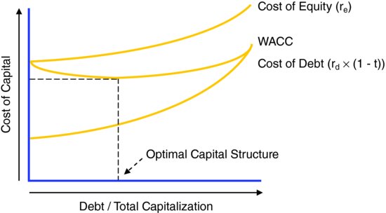
EXHIBIT 3.14 Optimal Capital Structure
Step III(b): Estimate Cost of Debt (rd)
A company's cost of debt reflects its credit profile at the target capital structure, which is based on a multitude of factors including size, sector, outlook, cyclicality, credit ratings, credit statistics, cash flow generation, financial policy, and acquisition strategy, among others. Assuming the company is currently at its target capital structure, cost of debt is generally derived from the blended yield on its outstanding debt instruments, which may include a mix of public and private debt. In the event the company is not currently at its target capital structure, the cost of debt must be derived from peer companies.
For publicly traded bonds, cost of debt is determined on the basis of the current yield14 on all outstanding issues. For private debt, such as revolving credit facilities and term loans,15 the banker typically consults with an in-house debt capital markets (DCM) specialist to ascertain the current yield. Market-based approaches such as these are generally preferred as the current yield on a company's outstanding debt serves as the best indicator of its expected cost of debt and reflects the risk of default. Bond quotes and key terms are available through the Bloomberg Bond Description function DES<GO> (see Appendix 3.2).
In the absence of current market data (e.g., for companies with debt that is not actively traded), an alternative approach is to calculate the company's weighted average cost of debt on the basis of the at-issuance coupons of its current debt maturities. This approach, however, is not always accurate as it is backward-looking and may not reflect the company's cost of raising debt capital under prevailing market conditions. A preferred, albeit more time-consuming, approach in these instances is to approximate a company's cost of debt based on its current (or implied) credit ratings at the target capital structure and the cost of debt for comparable credits, typically with guidance from an in-house DCM professional.
Once determined, the cost of debt is tax-effected at the company's marginal tax rate as interest payments are tax deductible.
Step III(c): Estimate Cost of Equity (re)
Cost of equity is the required annual rate of return that a company's equity investors expect to receive (including dividends). Unlike the cost of debt, which can be deduced from a company's outstanding maturities, a company's cost of equity is not readily observable in the market. To calculate the expected return on a company's equity, the banker typically employs a formula known as the capital asset pricing model (CAPM).
Capital Asset Pricing Model
CAPM is based on the premise that equity investors need to be compensated for their assumption of systematic risk in the form of a risk premium, or the amount of market return in excess of a stated risk-free rate. Systematic risk is the risk related to the overall market, which is also known as non-diversifiable risk. A company's level of systematic risk depends on the covariance of its share price with movements in the overall market, as measured by its beta (β) (discussed later in this section).
By contrast, unsystematic or “specific” risk is company- or sector-specific and can be avoided through diversification. Hence, equity investors are not compensated for it (in the form of a premium). As a general rule, the smaller the company and the more specified its product offering, the higher its unsystematic risk.
The formula for the calculation of CAPM is shown in Exhibit 3.15.

EXHIBIT 3.15 Calculation of CAPM
- where: rf = risk-free rate
- βL = levered beta
- rm = expected return on the market
- rm – rf = market risk premium
Risk-Free Rate (rf)
The risk-free rate is the expected rate of return obtained by investing in a “riskless” security. U.S. government securities such as T-bills, T-notes, and T-bonds16 are accepted by the market as “risk-free” because they are backed by the full faith of the U.S. federal government. Interpolated yields17 for government securities can be located on Bloomberg18 as well as the U.S. Department of Treasury website,19 among others. Bloomberg also provides a U.S. Treasury Interpolated Benchmark Monitor which displays yields for 1 month to 30-year treasuries (USTI<GO>, see Appendix 3.3). The actual risk-free rate used in CAPM varies with the prevailing yields for the chosen security.
Investment banks may differ on accepted proxies for the appropriate risk-free rate, with many using the yield on the 10-year U.S. Treasury note and others preferring the yield on longer-term Treasuries. The general goal is to use as long-dated an instrument as possible to match the expected life of the company (assuming a going concern), but practical considerations also need to be taken into account. Due to the moratorium on the issuance of 30-year Treasury bonds20 and shortage of securities with 30-year maturities, Ibbotson Associates (“Ibbotson”)21 uses an interpolated yield for a 20-year bond as the basis for the risk-free rate.22,23
Market Risk Premium (rm – rf or mrp)
The market risk premium is the spread of the expected market return24 over the risk-free rate. Finance professionals, as well as academics, often differ over which historical time period is most relevant for observing the market risk premium. Some believe that more recent periods, such as the last ten years or the post–World War II era are more appropriate, while others prefer to examine the pre–Great Depression era to the present.
Ibbotson tracks data on the equity risk premium dating back to 1926. Depending on which time period is referenced, the premium of the market return over the risk-free rate (rm – rf) may vary substantially. For the 1926 to 2011 period, Ibbotson calculates a market risk premium of 6.62%.25
Many investment banks have a firm-wide policy governing market risk premium in order to ensure consistency in valuation work across their various projects and departments. The equity risk premium employed on Wall Street typically ranges from approximately 5% to 8%. Consequently, it is important for the banker to consult with senior colleagues for guidance on the appropriate market risk premium to use in the CAPM formula. For shorter duration calculations of market risk premium, Bloomberg provides functionality via function: EQRP<GO>.
Beta (β)
Beta is a measure of the covariance between the rate of return on a company's stock and the overall market return (systematic risk), with the S&P 500 traditionally used as a proxy for the market. As the S&P 500 has a beta of 1.0, a stock with a beta of 1.0 should have an expected return equal to that of the market. A stock with a beta of less than 1.0 has lower systematic risk than the market, and a stock with a beta greater than 1.0 has higher systematic risk. Mathematically, this is captured in the CAPM, with a higher beta stock exhibiting a higher cost of equity; and vice versa for lower beta stocks.
A public company's historical beta may be sourced from financial information resources such as Bloomberg via function: BETA<GO> (see Appendix 3.4). Recent historical equity returns (i.e., over the previous two to five years), however, may not be a reliable indicator of future returns. Therefore, many bankers prefer to use a predicted beta such as the Bloomberg “Adjusted Beta” whenever possible as it is meant to be forward-looking.
The exercise of calculating WACC for a private company involves deriving beta from a group of publicly traded peer companies that may or may not have similar capital structures to one another or the target. To neutralize the effects of different capital structures (i.e., remove the influence of leverage), the banker must unlever the beta for each company in the peer group to achieve the asset beta (“unlevered beta”).
The formula for unlevering beta is shown in Exhibit 3.16.

EXHIBIT 3.16 Unlevering Beta
- where: βU = unlevered beta
- βL = levered beta
- D/E = debt-to-equity26 ratio
- t = marginal tax rate
After calculating the unlevered beta for each company, the banker determines the average unlevered beta for the peer group.27 This average unlevered beta is then relevered using the company's target capital structure and marginal tax rate. The formula for relevering beta is shown in Exhibit 3.17.

EXHIBIT 3.17 Relevering Beta
- where: D/E = target debt-to-equity ratio
The resulting levered beta serves as the beta for calculating the private company's cost of equity using the CAPM. Similarly, for a public company that is not currently at its target capital structure, its asset beta must be calculated and then relevered at the target D/E.
Size Premium (SP)
The concept of a size premium is based on empirical evidence suggesting that smaller-sized companies are riskier and, therefore, should have a higher cost of equity. This phenomenon, which to some degree contradicts the CAPM, relies on the notion that smaller companies' risk is not entirely captured in their betas given limited trading volumes of their stock, making covariance calculations inexact. Therefore, the banker may choose to add a size premium to the CAPM formula for smaller companies to account for the perceived higher risk and, therefore, expected higher return (see Exhibit 3.18). Ibbotson provides size premia for companies based on their market capitalization, tiered in deciles.

EXHIBIT 3.18 CAPM Formula Adjusted for Size Premium
- where: SP = size premium
Step III(d): Calculate WACC
Once all of the above steps are completed, the various components are entered into the formula in Exhibit 3.19 to calculate the company's WACC. In addition, Bloomberg provides a WACC analysis via function: WACC<GO> (see Appendix 3.5). Given the numerous assumptions involved in determining a company's WACC and its sizeable impact on valuation, its key inputs are typically sensitized to produce a WACC range (see Exhibit 3.49). This range is then used in conjunction with other sensitized inputs, such as exit multiple, to produce a valuation range for the target.

EXHIBIT 3.19 WACC Formula
STEP IV. DETERMINE TERMINAL VALUE
The DCF approach to valuation is based on determining the present value of all future FCF produced by a company. As it is infeasible to project a company's FCF indefinitely, the banker uses a terminal value to capture the value of the company beyond the projection period. As its name suggests, terminal value is typically calculated on the basis of the company's FCF (or a proxy such as EBITDA) in the final year of the projection period.
The terminal value typically accounts for a substantial portion of a company's value in a DCF, sometimes as much as three-quarters or more. Therefore, it is important that the company's terminal year financial data represents a steady state level of financial performance, as opposed to a cyclical high or low. Similarly, the underlying assumptions for calculating the terminal value must be carefully examined and sensitized.
There are two widely accepted methods used to calculate a company's terminal value—the exit multiple method and the perpetuity growth method. Depending on the situation and company being valued, the banker may use one or both methods, with each serving as a check on the other.
Exit Multiple Method
The EMM calculates the remaining value of a company's FCF produced after the projection period on the basis of a multiple of its terminal year EBITDA (or EBIT). This multiple is typically based on the current LTM trading multiples for comparable companies. As current multiples may be affected by sector or economic cycles, it is important to use both a normalized trading multiple and EBITDA. The use of a peak or trough multiple and/or an un-normalized EBITDA level can produce a skewed result. This is especially important for companies in cyclical industries.
As the exit multiple is a critical driver of terminal value, and hence overall value in a DCF, the banker subjects it to sensitivity analysis. For example, if the selected exit multiple range based on comparable companies is 7.0x to 8.0x, a common approach would be to create a valuation output table premised on exit multiples of 6.5x, 7.0x, 7.5x, 8.0x, and 8.5x (see Exhibit 3.32). The formula for calculating terminal value using the EMM is shown in Exhibit 3.20.

EXHIBIT 3.20 Exit Multiple Method
- where: n = terminal year of the projection period
Perpetuity Growth Method
The PGM calculates terminal value by treating a company's terminal year FCF as a perpetuity growing at an assumed rate. As the formula in Exhibit 3.21 indicates, this method relies on the WACC calculation performed in Step III and requires the banker to make an assumption regarding the company's long-term, sustainable growth rate (“perpetuity growth rate”). The perpetuity growth rate is typically chosen on the basis of the company's expected long-term industry growth rate, which generally tends to be within a range of 2% to 4% (i.e., nominal GDP growth). As with the exit multiple, the perpetuity growth rate is also sensitized to produce a valuation range.

EXHIBIT 3.21 Perpetuity Growth Method
- where: FCF = unlevered free cash flow
- n = terminal year of the projection period
- g = perpetuity growth rate
- r = WACC
The PGM is often used in conjunction with the EMM, with each serving as a sanity check on the other. For example, if the implied perpetuity growth rate, as derived from the EMM is too high or low (see Exhibits 3.22(a) and 3.22(b)), it could be an indicator that the exit multiple assumptions are unrealistic.

EXHIBIT 3.22(a) Implied Perpetuity Growth Rate (End-of-Year Discounting)

EXHIBIT 3.22(b) Implied Perpetuity Growth Rate (Mid-Year Discounting, see Exhibit 3.26)
(a)Terminal Value calculated using the EMM.
Similarly, if the implied exit multiple from the PGM (see Exhibits 3.23(a) and 3.23(b)) is not in line with normalized trading multiples for the target or its peers, the perpetuity growth rate should be revisited.

EXHIBIT 3.23(a) Implied Exit Multiple (End-of-Year Discounting)

EXHIBIT 3.23(b) Implied Exit Multiple (Mid-Year Discounting, see Exhibit 3.26))
(a)Terminal Value calculated using the PGM.
STEP V. CALCULATE PRESENT VALUE AND DETERMINE VALUATION
Calculate Present Value
Calculating present value centers on the notion that a dollar today is worth more than a dollar tomorrow, a concept known as the time value of money. This is due to the fact that a dollar earns money through investments (capital appreciation) and/or interest (e.g., in a money market account). In a DCF, a company's projected FCF and terminal value are discounted to the present at the company's WACC in accordance with the time value of money.
The present value calculation is performed by multiplying the FCF for each year in the projection period and the terminal value by its respective discount factor. The discount factor is the fractional value representing the present value of one dollar received at a future date given an assumed discount rate. For example, assuming a 10% discount rate, the discount factor for one dollar received at the end of one year is 0.91 (see Exhibit 3.24).

EXHIBIT 3.24 Discount Factor
where: n = year in the projection period
The discount factor is applied to a given future financial statistic to determine its present value. For example, given a 10% WACC, FCF of $100 million at the end of the first year of a company's projection period (Year 1) would be worth $91 million today (see Exhibit 3.25).

EXHIBIT 3.25 Present Value Calculation Using a Year-End Discount Factor
where: n = year in the projection period
Mid-Year Convention
To account for the fact that annual FCF is usually received throughout the year rather than at year-end, it is typically discounted in accordance with a mid-year convention. Mid-year convention assumes that a company's FCF is received evenly throughout the year, thereby approximating a steady (and more realistic) FCF generation.28
The use of a mid-year convention results in a slightly higher valuation than year-end discounting due to the fact that FCF is received sooner. As Exhibit 3.26 depicts, if one dollar is received evenly over the course of the first year of the projection period rather than at year-end, the discount factor is calculated to be 0.95 (assuming a 10% discount rate). Hence, $100 million received throughout Year 1 would be worth $95 million today in accordance with a mid-year convention, as opposed to $91 million using the year-end approach in Exhibit 3.25.

EXHIBIT 3.26 Discount Factor Using a Mid-Year Convention
- where: n = year in the projection period
- 0.5 = is subtracted from n in accordance with a mid-year convention
Terminal Value Considerations
When employing a mid-year convention for the projection period, mid-year discounting is also applied for the terminal value under the PGM, as the banker is discounting perpetual future FCF assumed to be received throughout the year. The EMM, however, which is typically based on the LTM trading multiples of comparable companies for a calendar year end EBITDA (or EBIT), uses year-end discounting.
Determine Valuation
Calculate Enterprise Value
A company's projected FCF and terminal value are each discounted to the present and summed to provide an enterprise value. Exhibit 3.27 depicts the DCF calculation of enterprise value for a company with a five-year projection period, incorporating a mid-year convention and the EMM.

EXHIBIT 3.27 Enterprise Value Using Mid-Year Discounting
Derive Implied Equity Value
To derive implied equity value, the company's net debt, preferred stock, and noncontrolling interest are subtracted from the calculated enterprise value (see Exhibit 3.28).

EXHIBIT 3.28 Equity Value
Derive Implied Share Price
For publicly traded companies, implied equity value is divided by the company's fully diluted shares outstanding to calculate an implied share price (see Exhibit 3.29).

EXHIBIT 3.29 Share Price
The existence of in-the-money options and warrants, however, creates a circular reference in the basic formula shown in Exhibit 3.29 between the company's fully diluted shares outstanding count and implied share price. In other words, equity value per share is dependent on the number of fully diluted shares outstanding, which, in turn, is dependent on the implied share price. This is remedied in the model by activating the iteration function in Microsoft Excel (see Exhibit 3.30).

EXHIBIT 3.30 Iteration Function in Microsoft Excel
Once the iteration function is activated, the model is able to iterate between the cell determining the company's implied share price (see shaded area “A” in Exhibit 3.31) and those cells determining whether each option tranche is in-the-money (see shaded area “B” in Exhibit 3.31). At an assumed enterprise value of $6,000 million, implied equity value of $4,500 million, 80 million basic shares outstanding, and the options data shown in Exhibit 3.31, we calculate an implied share price of $55.00.

EXHIBIT 3.31 Calculation of Implied Share Price
Perform Sensitivity Analysis
The DCF incorporates numerous assumptions, each of which can have a sizeable impact on valuation. As a result, the DCF output is viewed in terms of a valuation range based on a series of key input assumptions, rather than as a single value. The exercise of deriving a valuation range by varying key inputs is called sensitivity analysis.
Sensitivity analysis is a testament to the notion that valuation is as much an art as a science. Key valuation drivers such as WACC, exit multiple, and perpetuity growth rate are the most commonly sensitized inputs in a DCF. The banker may also perform additional sensitivity analysis on key financial performance drivers, such as sales growth rates and profit margins (e.g., EBITDA or EBIT). Valuation outputs produced by sensitivity analysis are typically displayed in a data table, such as that shown in Exhibit 3.32.
The center shaded portion of the sensitivity table in Exhibit 3.32 displays an enterprise value range of $5,598 million to $6,418 million assuming a WACC range of 9.5% to 10.5% and an exit multiple range of 7x to 8x. As the exit multiple increases, enterprise value increases accordingly; conversely, as the discount rate increases, enterprise value decreases.

EXHIBIT 3.32 Sensitivity Analysis
As with comparable companies and precedent transactions, once a DCF valuation range is determined, it should be compared to the valuation ranges derived from other methodologies. If the output produces notably different results, it is advisable to revisit the assumptions and fine-tune, if necessary. Common missteps that can skew the DCF valuation include the use of unrealistic financial projections (which generally has the largest impact),29 WACC, or terminal value assumptions. A substantial difference in the valuation implied by the DCF versus other methodologies, however, does not necessarily mean the analysis is flawed. Multiples-based valuation methodologies may fail to account for company-specific factors that may imply a higher or lower valuation.
KEY PROS AND CONS
Pros
- Cash flow-based – reflects value of projected FCF, which represents a more fundamental approach to valuation than using multiples-based methodologies
- Market independent – more insulated from market aberrations such as bubbles and distressed periods
- Self-sufficient – does not rely entirely upon truly comparable companies or transactions, which may or may not exist, to frame valuation; a DCF is particularly important when there are limited or no “pure play” public comparables to the company being valued
- Flexibility – allows the banker to run multiple financial performance scenarios, including improving or declining growth rates, margins, capex requirements, and working capital efficiency
Cons
- Dependence on financial projections – accurate forecasting of financial performance is challenging, especially as the projection period lengthens
- Sensitivity to assumptions – relatively small changes in key assumptions, such as growth rates, margins, WACC, or exit multiple, can produce meaningfully different valuation ranges
- Terminal value – the present value of the terminal value can represent as much as three-quarters or more of the DCF valuation, which decreases the relevance of the projection period's annual FCF
- Assumes constant capital structure – basic DCF does not provide flexibility to change the company's capital structure over the projection period
ILLUSTRATIVE DISCOUNTED CASH FLOW ANALYSIS FOR VALUECO
The following section provides a detailed, step-by-step construction of a DCF analysis and illustrates how it is used to establish a valuation range for our target company, ValueCo. As discussed in the Introduction, ValueCo is a private company for which we are provided detailed historical financial information. However, for our illustrative DCF analysis, we assume that no management projections were provided in order to cultivate the ability to develop financial projections with limited information. We do, however, assume that we were provided with basic information on ValueCo's business and operations.
Step I. Study the Target and Determine Key Performance Drivers
As a first step, we reviewed the basic company information provided on ValueCo. This foundation, in turn, allowed us to study ValueCo's sector in greater detail, including the identification of key competitors (and comparable companies), customers, and suppliers. Various trade journals and industry studies, as well as SEC filings and research reports of public comparables, were particularly important in this respect.
From a financial perspective, ValueCo's historical financials provided a basis for developing our initial assumptions regarding future performance and projecting FCF. We used consensus estimates of public comparables to provide further guidance for projecting ValueCo's Base Case growth rates and margin trends.
Step II. Project Free Cash Flow
Historical Financial Performance
We began the projection of ValueCo's FCF by laying out its income statement through EBIT for the three-year historical and LTM periods (see Exhibit 3.33). We also entered ValueCo's historical capex and working capital data. The historical period provided important perspective for developing defensible Base Case projection period financials.
As shown in Exhibit 3.33, ValueCo's historical period includes financial data for 2009 to 2011 as well as for LTM 9/30/2012. The company's sales and EBITDA grew at a 10.9% and 16.9% CAGR, respectively, over the 2009 to 2011 period. In addition, ValueCo's EBITDA margin was in the approximately 19% to 21% range over this period, and average capex as a percentage of sales was 4.3%.
The historical working capital levels and ratios are also shown in Exhibit 3.33. ValueCo's average DSO, DIH, and DPO for the 2009 to 2011 period were 46.0, 102.8, and 40.0 days, respectively. For the LTM period, ValueCo's EBITDA margin was 20.7% and capex as a percentage of sales was 4.5%.

EXHIBIT 3.33 ValueCo Summary Historical Operating and Working Capital Data
Projection of Sales, EBITDA, and EBIT
Sales Projections
We projected ValueCo's top line growth for the first three years of the projection period on the basis of consensus research estimates for public comparable companies. Using the average projected sales growth rate for ValueCo's closest peers, we arrived at 2013E, 2014E, and 2015E YoY growth rates of 7.5%, 6%, and 5%, respectively, which are consistent with its historical rates.30 These growth rate assumptions (as well as the assumptions for all of our model inputs) formed the basis for the Base Case financial projections and were entered into an assumptions page that drives the DCF model (see Chapter 5, Exhibits 5.52 and 5.53).
As the projections indicate, Wall Street expects ValueCo's peers (and, by inference, we expect ValueCo) to continue to experience steady albeit declining growth through 2015E. Beyond 2015E, in the absence of additional company-specific information or guidance, we decreased ValueCo's growth to a sustainable long-term rate of 3% for the remainder of the projection period.

COGS and SG&A Projections
As shown in Exhibit 3.35, we held COGS and SG&A constant at the prior historical year levels of 60% and 19% of sales, respectively. Accordingly, ValueCo's gross profit margin remains at 40% throughout the projection period.

EXHIBIT 3.35 ValueCo Historical and Projected COGS and SG&A
EBITDA Projections
In the absence of guidance or management projections for EBITDA, we simply held ValueCo's margins constant throughout the projection period at prior historical year levels. These constant margins fall out naturally due to the fact that we froze COGS and SG&A as a percentage of sales at 2011 levels. As shown in Exhibit 3.36, ValueCo's EBITDA margins remain constant at 21% throughout the projection period. We also examined the consensus estimates for ValueCo's peer group, which provided comfort that the assumption of constant EBITDA margins was justifiable.

EXHIBIT 3.36 ValueCo Historical and Projected EBITDA
EBIT Projections
To drive EBIT projections, we held D&A as a percentage of sales constant at the 2011 level of 6%. We gained comfort that these D&A levels were appropriate as they were consistent with historical data as well as our capex projections (see Exhibit 3.39). EBIT was then calculated in each year of the projection period by subtracting D&A from EBITDA (see Exhibit 3.37). As previously discussed, an alternative approach is to construct the DCF on the basis of EBITDA and EBIT projections, with D&A simply calculated by subtracting EBIT from EBITDA.

EXHIBIT 3.37 ValueCo Historical and Projected EBIT
Projection of Free Cash Flow
Tax Projections
We calculated tax expense for each year at ValueCo's marginal tax rate of 38%. This tax rate was applied on an annual basis to EBIT to arrive at EBIAT (see Exhibit 3.38).

EXHIBIT 3.38 ValueCo Projected Taxes
Capex Projections
We projected ValueCo's capex as a percentage of sales in line with historical levels. As shown in Exhibit 3.39, this approach led us to hold capex constant throughout the projection period at 4.5% of sales. Based on this assumption, capex increases from $166.9 million in 2013E to $199 million in 2017E.

EXHIBIT 3.39 ValueCo Historical and Projected Capex
Change in Net Working Capital Projections
As with ValueCo's other financial performance metrics, historical working capital levels normally serve as reliable indicators of future performance. The direct prior year's ratios are typically the most indicative provided they are consistent with historical levels. This was the case for ValueCo's 2011 working capital ratios, which we held constant throughout the projection period (see Exhibit 3.40).

EXHIBIT 3.40 ValueCo Historical and Projected Net Working Capital
For A/R, inventory, and A/P, respectively, these ratios are DSO of 47.6, DIH of 105.8, and DPO of 37.9. For prepaid expenses and other current assets, accrued liabilities, and other current liabilities, the percentage of sales levels are 5.1%, 8.0%, and 2.9%, respectively. For ValueCo's Base Case financial projections, we conservatively did not assume any improvements in working capital efficiency during the projection period.
As depicted in the callouts in Exhibit 3.40, using ValueCo's 2011 ratios, we projected 2012E NWC to be $635 million. To determine the 2013E YoY change in NWC, we then subtracted this value from ValueCo's 2013E NWC of $682.6 million. The $47.6 million difference is a use of cash and is, therefore, subtracted from EBIAT, resulting in a reduction of ValueCo's 2013E FCF. Hence, it is shown in Exhibit 3.41 as a negative value.

EXHIBIT 3.41 ValueCo's Projected Changes in Net Working Capital
The methodology for determining ValueCo's 2013E NWC was then applied in each year of the projection period. Each annual change in NWC was added to the corresponding annual EBIAT (with increases in NWC expressed as negative values) to calculate annual FCF.
A potential shortcut to the detailed approach outlined in Exhibits 3.40 and 3.41 is to bypass projecting individual working capital components and simply project NWC as a percentage of sales in line with historical levels. For example, we could have used ValueCo's 2011 NWC percentage of sales ratio of 18.4% to project its NWC for each year of the projection period. We would then have simply calculated YoY changes in ValueCo's NWC and made the corresponding subtractions from EBIAT.
Free Cash Flow Projections
Having determined all of the above line items, we calculated ValueCo's annual projected FCF, which increases from $353.3 million in 2013E to $454.2 million in 2017E (see Exhibit 3.42).

EXHIBIT 3.42 ValueCo Projected FCF
Step III. Calculate Weighted Average Cost of Capital
Below, we demonstrate the step-by-step calculation of ValueCo's WACC, which we determined to be 10%.
Step III(a): Determine Target Capital Structure
Our first step was to determine ValueCo's target capital structure. For private companies, the target capital structure is generally extrapolated from peers. As ValueCo's peers have an average (mean) D/E of 42.9%—or debt-to-total capitalization (D/(D+E)) of 30%—we used this as our target capital structure (see Exhibit 3.45).
Step III(b): Estimate Cost of Debt
We estimated ValueCo's long-term cost of debt based on the current yields on its existing term loan and senior notes (see Exhibit 3.43).31 The term loan, which for illustrative purposes we assumed is trading at par, is priced at a spread of 350 basis points (bps)32 to LIBOR33 (L+350 bps) with a LIBOR floor of 1% (see Chapter 4). The senior notes are also assumed to be trading at par and have a coupon of 8%. Based on the rough average cost of debt across ValueCo's capital structure, we estimated ValueCo's cost of debt at 6% (or approximately 3.7% on an after-tax basis).

EXHIBIT 3.43 ValueCo Capitalization
Step III(c): Estimate Cost of Equity
We calculated ValueCo's cost of equity in accordance with the CAPM formula shown in Exhibit 3.44.

EXHIBIT 3.44 CAPM Formula
Determine Risk-free Rate and Market Risk Premium
We assumed a risk-free rate (rf) of 3% based on the interpolated yield of the 20-year Treasury bond. For the market risk premium (rm – rr), we used the arithmetic mean of 6.62% (for the 1926–2011 period) in accordance with Ibbotson.
Determine the Average Unlevered Beta of ValueCo's Comparable Companies
As ValueCo is a private company, we extrapolated beta from its closest comparables (see Chapter 1). We began by sourcing predicted levered betas for each of ValueCo's closest comparables.34 We then entered the market values for each comparable company's debt35 and equity, and calculated the D/E ratios accordingly. This information, in conjunction with the marginal tax rate assumptions, enabled us to unlever the individual betas and calculate an average unlevered beta for the peer group (see Exhibit 3.45).

EXHIBIT 3.45 Average Unlevered Beta
For example, based on Sherman Co.'s predicted levered beta of 1.35, D/E of 56.3%, and a marginal tax rate of 38%, we calculated an unlevered beta of 1.00. We performed this calculation for each of the selected comparable companies and then calculated an average unlevered beta of 1.02 for the group.
Relever Average Unlevered Beta at ValueCo's Capital Structure
We then relevered the average unlevered beta of 1.02 at ValueCo's previously determined target capital structure of 42.9% D/E, using its marginal tax rate of 38%. This provided a levered beta of 1.29 (see Exhibit 3.46).

EXHIBIT 3.46 ValueCo Relevered Beta
Calculate Cost of Equity
Using the CAPM, we calculated a cost of equity for ValueCo of 12.7% (see Exhibit 3.47), which is higher than the expected return on the market (calculated as 9.6% based on a risk-free rate of 3% and a market risk premium of 6.62%). This relatively high cost of equity was driven by the relevered beta of 1.29, versus 1.0 for the market as a whole, as well as a size premium of 1.14%.36

EXHIBIT 3.47 ValueCo Cost of Equity
Step III(d): Calculate WACC
We now have determined all of the components necessary to calculate ValueCo's WACC. These inputs were entered into the formula in Exhibit 3.12, resulting in a WACC of 10%. Exhibit 3.48 displays each of the assumptions and calculations for determining ValueCo's WACC.
As previously discussed, the DCF is highly sensitive to WACC, which itself is dependent on numerous assumptions governing target capital structure, cost of debt, and cost of equity. Therefore, a sensitivity analysis is typically performed on key WACC inputs to produce a WACC range. In Exhibit 3.49, we sensitized target capital structure and pre-tax cost of debt to produce a WACC range of approximately 9.5% to 10.5% for ValueCo.

EXHIBIT 3.48 ValueCo WACC Calculation

EXHIBIT 3.49 ValueCo Weighted Average Cost of Capital Analysis
Step IV. Determine Terminal Value
Exit Multiple Method
We used the LTM EV/EBITDA trading multiples for ValueCo's closest public comparable companies as the basis for calculating terminal value in accordance with the EMM. These companies tend to trade in a range of 7.0x to 8.0x LTM EBITDA. Multiplying ValueCo's terminal year EBITDA of $929.2 million by the 7.5x midpoint of this range provided a terminal value of $6,969 million (see Exhibit 3.50).

EXHIBIT 3.50 Exit Multiple Method
We then solved for the perpetuity growth rate implied by the exit multiple of 7.5x EBITDA. Given the terminal year FCF of $454.2 million and 10% midpoint of the selected WACC range, and adjusting for the use of a mid-year convention for the PGM terminal value, we calculated an implied perpetuity growth rate of 3% (see Exhibit 3.51).

EXHIBIT 3.51 Implied Perpetuity Growth Rate
Perpetuity Growth Method
We selected a perpetuity growth rate range of 2% to 4% to calculate ValueCo's terminal value using the PGM. Using a perpetuity growth rate midpoint of 3%, WACC midpoint of 10%, and terminal year FCF of $454.2 million, we calculated a terminal value of $6,683.8 million for ValueCo (see Exhibit 3.52).

EXHIBIT 3.52 Perpetuity Growth Rate
The terminal value of $6,683.8 million calculated using the PGM implied a 7.5x exit multiple, adjusting for year-end discounting using the EMM (see Exhibit 3.53). This is consistent with our assumptions using the EMM approach in Exhibit 3.50.

EXHIBIT 3.53 Implied Exit Multiple
Step V. Calculate Present Value and Determine Valuation
Calculate Present Value
ValueCo's projected annual FCF and terminal value were discounted to the present using the selected WACC midpoint of 10% (see Exhibit 3.54). We used a mid-year convention to discount projected FCF. For the terminal value calculation using the EMM, however, we used year-end discounting.

EXHIBIT 3.54 Present Value Calculation
Determine Valuation
Calculate Enterprise Value
The results of the present value calculations for the projected FCF and terminal value were summed to produce an enterprise value of $5,926.4 million for ValueCo (see Exhibit 3.55). The enterprise value is comprised of $1,599.2 million from the present value of the projected FCF and $4,327.2 million from the present value of the terminal value. This implies that ValueCo's terminal value represents 73% of the enterprise value.

EXHIBIT 3.55 Enterprise Value
Derive Equity Value
We then calculated an implied equity value of $4,676.4 million for ValueCo by subtracting its net debt of $1,250 million ($1,500 million of debt – $250 million of cash) from enterprise value of $5,926.4 million (Exhibit 3.56). If ValueCo were a publicly traded company, we would then have divided the implied equity value by its fully diluted shares outstanding to determine an implied share price (see Exhibits 3.2 and 3.31).

EXHIBIT 3.56 Equity Value
DCF Output Page
Exhibit 3.57 displays a typical DCF output page for ValueCo using the EMM.

EXHIBIT 3.57 ValueCo DCF Analysis Output Page
Perform Sensitivity Analysis
We then performed a series of sensitivity analyses on WACC and exit multiple for several key outputs, including enterprise value, equity value, implied perpetuity growth rate, implied EV/LTM EBITDA, and PV of terminal value as a percentage of enterprise value (see Exhibit 3.58).

EXHIBIT 3.58 ValueCo Sensitivity Analysis
We also sensitized key financial assumptions, such as sales growth rates and EBIT margins, to analyze the effects on enterprise value. This sensitivity analysis provided helpful perspective on our assumptions and enabled us to study the potential value creation or erosion resulting from outperformance or underperformance versus the Base Case financial projections. For example, as shown in Exhibit 3.59, an increase in ValueCo's annual sales growth rates and EBIT margins by 50 bps each results in an increase of approximately $179 million in enterprise value from $5,926 million to $6,105 million.

EXHIBIT 3.59 Sensitivity Analysis on Sales Growth Rates and EBIT Margins
After completing the sensitivity analysis, we proceeded to determine ValueCo's ultimate DCF valuation range. To derive this range, we focused on the shaded portion of the exit multiple / WACC data table (see top left corner of Exhibit 3.58). Based on an exit multiple range of 7.0x to 8.0x and a WACC range of 9.5% to 10.5%, we calculated an enterprise value range of approximately $5,530 million to $6,340 million for ValueCo.
We then added this range to our “football field” and compared it to the derived valuation ranges from our comparable companies analysis and precedent transactions analysis performed in Chapters 1 and 2 (see Exhibit 3.60).

EXHIBIT 3.60 ValueCo Football Field Displaying Comparable Companies, Precedent Transactions, and DCF Analysis
Bloomberg Appendix

APPENDIX 3.1 Reported Historical Figures and Consensus Estimates via Bloomberg Financial Analysis (FA<GO>)

APPENDIX 3.2 Bond Quote and Informational Overview from Bloomberg Bond Description Function (DES<GO>)

APPENDIX 3.3 U.S. Treasury Interpolated Benchmark Monitor (USTI<GO>)

APPENDIX 3.4 Historical Raw Beta and Adjusted Beta as Calculated by Bloomberg (BETA<GO>)

APPENDIX 3.5 Bloomberg WACC Analysis (WACC<GO>)