

Introduction to IBM Spectrum Conductor Deep Learning Impact
IBM Spectrum Conductor Deep Learning Impact (DLI) is built on IBM Spectrum Conductor with Spark, a highly available and resilient multi-tenant distributed framework, which provides Apache Spark and deep learning (DL) applications lifecycle support.
This chapter contains the following topics:
6.1 Definitions, acronyms, buzzwords, and abbreviations
Table 6-1 shows the terminologies that are used in this chapter.
Table 6-1 Some terminologies that are used in this chapter
|
Definitions
|
Description
|
|
IBM PowerAI
|
|
|
Inference
|
|
|
IBM Spectrum Conductor with Spark
|
IBM Spectrum Conductor with Spark enterprise platform.
|
|
Deep learning
|
A DL platform that is based on IBM Spectrum Conductor with Spark.
|
|
LMDB
|
Lightning Memory-Mapped Database, which is used by Caffe.
|
|
TFRecords
|
TFRecords is a commonly used TensorFlow training data format.
|
|
Parameter Server (PS)
|
|
|
Graphical processing unit (GPU)
|
|
|
NCCL
|
|
|
Hyperparameters tuning
|
When you train a neural network, a different hyperparameters setting of the model affects the training result, such as the time cost or the model performance. Hyperparameter optimization or tuning searches a set of optimal hyperparameters for a DL model that has the best performance.
|
|
Tree-structured Parzen Estimator Approach (TPE)
|
|
|
Random search
|
Search the best hyperparameter setting by randomly sampling settings from all possible candidates.
|
|
Bayesian optimization
|
Bayesian optimization is a methodology for the global optimization of noisy blackbox functions. For more information, see Practical Bayesian Optimization of Machine Learning Algorithms.
|
|
Underfitting
|
Underfitting refers to a model that cannot model the training data or generalize new data.
|
|
Overfitting
|
Overfitting refers to a model that models the training data too well.
|
|
Gradient explosion
|
Exploding gradients arise in deep networks when the gradients’ associating weights and the net’s error become too large.
|
|
Saturation
|
If the input of activation function is too large or too small, the gradients that are computed are so close to zero that learning either becomes slow or stops working.
|
6.2 Benefits of IBM Spectrum Conductor Deep Learning Impact
On IBM Power platforms, IBM PowerAI provides many DL frameworks and useful technologies for the customer to take advantages of and implement. In many cases, customers want to use DL technology and integrate with their existing applications to bring new value to their business. There are some important elements to ensure a (not one) DL project can be put into production successfully, such as data management, arithmetic and neural network management, and computing resource management.
Figure 6-1 demonstrates a general lifecycle for DL projects.

Figure 6-1 Data science of deep learning project lifecycle
A DL product always begins with the customer's business requirement (step 1). In most cases, data is provided by the customer. If you use a supervised training network, data labeling is needed too (step 2).
After you understand the business requirements and available data, you can implement one or more neural networks by completing the following high-level steps:
1. Reformatting or restructuring data to be in a usable/required format to be used by the model (step 3).
2. Import a DL network to create a training model (step 4).
3. Start a model training task (step 4).
4. Tune a model to improve accuracy (step 5).
5. Generate an inference model based on the trained model (step 6).
6. Integrate an inference model with a customer’s application (step 6 and 7).
7. Put the model into production (step 7).
8. Generate an updated inference model to adapt to changing data (step 8).
These steps explain a closed-loop lifecycle for DL projects.
DLI takes effect from step 3 - 8, except for step 7. DLI can provide other benefits:
•Multi-tenant support
•Manages GPU resources dynamically
•Training visualization
•Early stop warning during training
•Hyperparameter searching for model tuning
•Supports multiple-node training with fabric technology, which provides easier integration and better speed ratio
•Provide a RESTful API for a customer’s application to call an inference service
6.3 Key features of Deep Learning Impact
This section introduces some key features of DLI.
As a DL model development and management platform, the major targets of DLI are the following ones:
•To improve the accuracy of the neural network model
•To improve the training efficiency while processing a large-scale data set
•To provide real-time response for a user clients inference request after the model is deployed
To achieve these targets, DLI provides parallel data processing, hyperparameter tuning, parallel training with optimized gradient and weight reducing algorithm, training advisor, inference as service functions, and others.
6.3.1 Parallel data set processing
A DLI data set is used for model tuning, training, testing, and validation. Data set management features can help with a user management data set. A DLI data set can create, remove, and list data sets, monitor a data set’s status, and view data set details. It can support and manage the following data set types:
•LMDB and TFRecords
•Images for classification
•Images for object detection
•Images vector
•CSV data
•Raw data
When creating a data set, DLI can:
•Randomly shuffle the data
•Split a data set to train data set, test data set, and validate data set
•Resize images
•Convert data to LMDB or TFRecords
6.3.2 Monitoring and Optimization for one training model
The function is used for training process monitoring and issue detection. Training a deep neural network is complex and time-consuming, so it is important to know the current progress and status of a user’s training job. Monitoring and Optimization (MAO) provides the following features:
•Monitor the DL training job by capturing logs from instrumented underlying DL frameworks (filtering the logs based on keywords).
•Visualize the training progress by summarizing the training job’s monitoring data.
•Advise and optimize the training (enables the user to accept them and have it implement the optimizations on their behalf).
The training visualization feature can visualize run time, iteration, loss, and accuracy metrics as histograms of weights, activations, and gradients of the neural network. From these charts, the user knows whether the training is running smoothly or there is something wrong.
During the training process, MAO can help the user detect the following issues of neural network model design:
•Gradient explosion
•Overflow
•Saturation
•Divergence
•Overfitting
•Underfitting
If DLI detects any of these issues, DLI estimates whether the training process can skip the issue. If not, DLI provides an early stop suggestion and the amendment suggestion to the user. The user can stop the training, adjust the model, and start again. The function helps the user improve the tuning model efficiency.
6.3.3 Hyperparameter optimization and search
Hyperparameters are parameters whose values are set before the start of the model training process. DL models such as convolutional neural networks (CNNs) and recurrent neural networks (RNNs) can have 10 - 100 hyperparameters, for example, the learning rate, the regulations, and others. These parameters affect the model training process and the final model performance. Hyperparameters optimization is one of the direct impediments to tuning DL models. There are three algorithms to automatically optimize the hyperparameters: Random search, TPE, and Bayesian optimization based on the Gaussian Process.
Random search
This method is the most popular search method in machine learning (ML) and DL. It easily supports parallel jobs with high efficiency. If a user has the candidate value for the hyperparameters and they are discrete, random search is the best choice.
Tree-structured Parzen Estimator Approach search
This is a tree-based search method and the sampling window follows the Parzen estimator. This is a sequential search model, and during each search iteration, in parallel, it searches the potential optimization point. The TPE search efficiency is between the random search and the Bayesian search.
Bayesian search
This method is a traditional and high accuracy method to search hyperparameters. It uses Gaussian probability density to describe the relationship between hyperparameters and loss value of neural networks, and takes advantage of the Expectation Maximization (EM) algorithm to constantly find the best result. Bayesian search is also a sequential search method, so it can be quickly convergent to the best optimal value.
Our implementation takes advantage of the state-of-art research results and the IBM Spectrum Conductor with Spark platform to efficiently parallel search the best set of hyperparameters that has the best final model performance.
6.3.4 IBM Fabric for distributed training
DLI uses IBM Fabric technology as part of its general distribution DL framework. IBM Fabric is a general distribution DL framework. The implementation provides comprehensive support for distribution DL across multiple GPUs and nodes. It provides compatibility with existing TensorFlow and Caffe models. IBM Fabric supports various parallelization schemes for a gradient descent method, which results in more than an 80% speedup ratio. Furthermore, IBM Fabric can efficiently scale out on IBM Spectrum Conductor with Spark clusters.
IBM Fabric mainly supports the following functions:
•Single Node, Multiple GPUs Training is supported without PS for TensorFlow and Caffe models.
•Multiple Nodes, Multiple GPUs Training is supported by PS for TensorFlow and Caffe models.
•Distribution synchronous and asynchronous training algorithms are supported for multi-nodes, including a synchronous gradient data control algorithm, an asynchronous gradient data control algorithm, a synchronous weight data control algorithm, and an asynchronous weight data control algorithm.
•NCCL is supported for broadcasting and reducing gradient and weight data across multiple GPUs.
•Continue training is supported by saving and restoring the training checkpoint and snapshot files.
6.3.5 IBM Fabric and auto-scaling
In addition to the distributed training engine with IBM Fabric, there is an added auto-scaling function that is available. The distributed training engine with IBM Fabric and auto-scaling function uses a fine-grained control for training. This is an alternative to the coarse-grained strategy, where the resource utilization is capped and no additional GPUs can be added to the training phase. With auto-scaling, the Spark scheduler distributes the task and the session scheduler dynamically issues resources from the resource manager, enabling more GPUs to be added.
In the reclaim case, the scheduler worker finishes the current training iteration, pushes the gradient on PS, and then exits and gracefully shuts down. In the scale-up case, the scheduler dynamic adds more workers to the training job to pick up the pending training iteration.
6.3.6 DLI inference model
This model puts the trained DL model into production, which is the most exciting moment for a data scientist. The DLI inference model function makes this step easy and efficient by just clicking several buttons in the portal. The inference model is also the most important way that a user can really benefit from the DL model. The IBM Spectrum Conductor with Spark DLI serves the data scientist and user by managing the inference model as a service in the IBM Spectrum Conductor with Spark cluster and provides access to the user with an advanced inference engine. Based on the powerful scheduling, elastic scaling, and efficient resource management features from IBM Spectrum Conductor with Spark, the inference request from the user can be serviced in IBM Spectrum Conductor with Spark DLI smoothly and efficiently.
The DLI inference model supports the following functions:
•Convert a trained model into an inference model.
•Create an inference model with pre-trained weight files.
•Infer from an IBM Spectrum Conductor with Spark DLI web portal and REST API.
•Manage an inference model and results from a web portal and REST API.
•Support an inference model preinstallation to reduce the response time and increase resource utilization.
•Provide large throughput.
•Support running in a large dynamic cluster.
6.3.7 Supporting a shared multi-tenant infrastructure
DLI is built on IBM Spectrum Conductor with Spark, which uses the IBM Enterprise Grid Orchestrator (IBM EGO) product to provide resource management and scheduling capabilities for Spark applications within the IBM Spectrum Conductor with Spark cluster.
IBM EGO also provides the underlying system infrastructure to enable multiple applications to operate within a shared multi-tenant infrastructure.
IBM EGO also provides the underlying system infrastructure to enable multiple applications to operate within a shared multi-tenant infrastructure.
|
Note: For more information, see IBM EGO.
|
Figure 6-2 shows the work flow to create a multi-tenant environment.

Figure 6-2 Creating a multi-tenant environment work flow
During the creation of the IBM EGO user, there are different authorities for one user. Figure 6-3 describes the role and authority in IBM Spectrum Conductor with Spark.

Figure 6-3 Different role and authority for one IBM EGO user
Within one IBM Spectrum Conductor with Spark cluster, there is a session scheduler role to dispatch resources for different tasks. There are three policies: Priority, FIFO, and Fairshare.
Figure 6-4 on page 151 shows the multi-tenant environment, and resource management for tenants and applications.

Figure 6-4 Multi-tenant resource management example
|
Note: To support the IBM Fabric and the auto-scaling function, set Fairshare for the schedule policy.
|
Multi-tenant example 1
Figure 6-5 is a straightforward scenario. In this scenario, there are two servers with their own CPU and GPU resources.

Figure 6-5 Multi-tenant example 1
The scenario has the following characteristics:
•The user creates a resource group for each host. Host1 has CPU_RG1 and GPU_RG1 resource groups and host2 has CPU_RG2 and GPU_RG2 resource groups.
•Consumer_1 includes CPU_RG1 and GPU_RG1 resource groups and tenant group 1 (Tenant_1, Tenant_2, and so on).
•Consumer_2 includes CPU_RG2 and GPU_RG2 resource groups and tenant group 2 (Tenant_a, Tenant_b, and so on).
•The Spark Instance Group (SIG) 1 includes consumer_1 and its resource groups. The SIG 2 includes consumer_2 and its resource groups.
With this kind of configuration, the two tenant groups use separate hardware resources for DL tasks, and can see only their own tasks.
Multi-tenant example 2
Figure 6-6 shows another sample scenario. In this scenario, there are two servers with their own CPU and GPU resources.

Figure 6-6 Multi-tenant example 2
The scenario has the following characteristics:
•All CPU resources of the two hosts are configured in one resource group: CPU_RG1.
•All GPU resources of the two hosts are configured in one resource group: GPU_RG.
•Consumer_1 includes the two resource groups and tenant group 1 (Tenant_1, Tenant_2, and so on).
•Consumer_2 includes the two resource groups and tenant group 2 (Tenant_a, Tenant_b, and so on).
•SIG 1 includes consumer_1 and the two resource groups.
•SIG 2 includes consumer_2 and the two resource groups.
With this kind of configuration, the two tenant groups share the hardware, and can see only their own DL tasks.
Multi-tenant example 3
Figure 6-7 is a simple example. In this scenario, there are two servers with their own CPU and GPU resources. The scenario has the following characteristics:
•All resources of host1 and host2 are configured into two resource groups: CPU_RG1 and GPU_RG2.
•All resources of host2 and host3 are configured into two resource groups: CPU_RG2 and GPU_RG2.
•Consumer_1 has CPU_RG1 and GPU_RG1 resource groups and tenant group 1 (Tenant_1, Tenant_2, and so on).
•Consumer_2 has CPU_RG2 and GPU_RG2 resource groups and tenant group 2 (Tenant_a, Tenant_b, and so on).
•SIG 1 includes consumer_1 and its resource groups.
•SIG 2 includes consumer_2 and its two resource groups.
With this kind of configuration, the two tenant groups share hardware of hosts2, but have their own hardware. The two tenant groups can see only their own DL tasks.

Figure 6-7 Multi-tenant example 3
6.4 DLI deployment
This section introduces how to deploy DLI on IBM PowerAI.
6.4.1 Deployment consideration
This section introduces three deployment modes: single node, multi-nodes without a high availability (HA) function, and multi-nodes with a HA function. In real case scenarios, there are some other methods, although they depend on the customer’s requirements.
Regarding this deployment model, this scenario focus on a general architecture. In our environment, the version of software stack is as follows:
•DLI V1.1
•IBM Spectrum Conductor with Spark V2.2.1
•IBM PowerAI V1.5
•RHEL for Power Systems (ppc64le) V7.4
•CUDA V9.0.176
•GPU driver V384.81
•CUDA Deep Neural Network (cuDNN) V7.0.4
•IBM Spectrum MPI V10.1
|
Note: You must use a fully qualified domain name (FQDN) to access the IBM Spectrum Conductor with Spark GUI. In a DLI solution, you use the FQDN too. Here is an example of a /etc/hosts file FQDN entry:
172.16.51.96 dli01.dli.com dli01
|
6.4.2 DLI single-node mode
In this mode, there is only one node. This mode is usually deployed for developing and testing purposes. The node acts as both master and compute roles. Figure 6-8 on page 155 shows the sequence of installation steps.

Figure 6-8 Installation steps for single node DLI environment
For explanation of the first three steps, see Chapter 4, “Deploying IBM PowerAI” on page 59.
After IBM PowerAI is installed, you can start the installation of IBM Spectrum Conductor with Spark and create a cluster. You also must install the required open source software. To obtain the installation script, see GitHub.
The DLI application itself can be installed next, and the GPU resource and SIGs can be configured. The environment is then ready for DL activities.
6.4.3 DLI cluster without a high availability function
In this mode, there are several nodes in the DLI cluster, and there is always one node that acts as the management node. In this case, this node acts as the master node too, as shown in Figure 6-9.

Figure 6-9 Topology of a DLI cluster without the high availability function
Figure 6-10 illustrates the typical installation steps for this configuration of the DLI cluster.

Figure 6-10 Installation steps for a DLI cluster without the high availability function enabled
6.4.4 DLI cluster with a high availability function
Figure 6-11 shows one topology where the HA function is enabled. The topology has two management nodes and two compute nodes.

Figure 6-11 Topology of DLI cluster with high availability function enabled
|
Note: If you want to enable the DLI HA function, do not configure GPU devices in the master nodes because if a workload is running on the master node and this node fails (although all IBM Spectrum Conductor with Spark and DLI services can be restarted on the master candidate node), the workload must be manually restarted because it abnormally ended.
|
Figure 6-12 on page 159 shows the installation steps for this kind of cluster.

Figure 6-12 Installation steps for a DLI cluster with the high availability function enabled
6.4.5 Binary files installation for the high availability enabled cluster
Before you install a HA enabled DLI cluster, you must consider where to place the IBM Spectrum Conductor with Spark and DLI files. The two typical options are locally or in a shared file system.
|
Note: The shared file system implementation is not described in this section. We assume that you have implemented a shared file system by using IBM Spectrum Scale™ or any file system of your preference.
|
Binary files in local disks
In this installation, all binary files are installed in a local file system, as shown in Figure 6-13. However, all configuration files and log files are installed in the shared file system.

Figure 6-13 An example of file system layout for location installation
|
Note: The /opt/ibm/spectrumcomputing directory is the default directory to place IBM Spectrum Conductor with Spark and DLI binary files. You can change it during the installation.
|
Binary files in shared file systems
Figure 6-13 illustrates an example installation for a HA enabled DLI cluster. During the installation sequence, you set one option to specify a target installation directory, which is in a shared file system. Then, all binary files and other files are installed in this shared file system, as shown in Figure 6-14 on page 161.

Figure 6-14 Shared file system installation
|
Note: The /sharefs/spectrumcomputing directory is an example shared file system for the IBM Spectrum Conductor with Spark installation.
The /sharefs/dli_userdata directory is an example of setting the shared file system during a DLI installation.
THe /sharefs/sig_share directory is an example of setting the shared file system during the SIG creation because it is used for the SIG HA function.
|
6.4.6 A DLI cluster with a high availability function installation guide
This section provides an overview about how to set up a DLI cluster and enable the HA feature.
Topology
In this case, the topology consists of three nodes: Two nodes are configured as management nodes, and one node is configured as the compute node. The two management nodes enable the HA function. The compute node runs the DL workload, as shown in Figure 6-15.

Figure 6-15 Topology of a DLI cluster
Regarding the binary files location, this example uses a local file system with a default value of /opt/ibm/spectrumcomputing.
Figure 6-16 on page 163 shows the installation steps for this configuration.

Figure 6-16 Installation steps
It is expected that the required operating system is installed and configured according to the installation guide and that IBM PowerAI itself is installed on all nodes.
Because HA DLI relies on the IBM Spectrum Conductor with Spark HA framework, do any required HA testing for IBM Spectrum Conductor with Spark before starting DLI. The HA tests must be repeated after the subsequent installation of DLI and again with a running DL workload.
Steps to install two management nodes
As shown in Example 6-1, some configuration is required across all the nodes before you begin the installation.
Example 6-1 Environment settings for all nodes
root@dli01:~# cat /etc/hosts
...
172.16.51.96 dli01.dli.com dli01
172.16.51.97 dli02.dli.com dli02
172.16.51.98 dli03.dli.com dli03
root@dli01:~# cat /etc/sysctl.conf
...
vm.max_map_count = 262144
root@dli01:~# useradd egoadmin -m
root@dli01:~# cat /etc/security/limits.conf
egoadmin soft nproc 65535
egoadmin hard nproc 65535
egoadmin soft nofile 65535
egoadmin hard nofile 65535
root - nproc 65536
root - nofile 65536
* - memlock unlimited
root@dli01:~# cat /etc/security/limits.d/20-nproc.conf
* soft nproc 4096
root soft nproc unlimited
egoadmin - nproc 65536
|
Note: Configuring the Network Time Protocol (NTP) is a requirement in a distributed multi-node environment.
|
In this example environment, we use a simple NFS mount as a shared file system. In a production environment, use IBM Spectrum Scale (or its equivalent) to provide the shared file system.
The detailed sequence of steps that are used to install and configure the two management nodes are documented in Table 6-2.
Table 6-2 Steps for management nodes installation
|
Operations on dli01 node
|
Operations on dli02 node
|
||
|
User
|
Operation
|
User
|
Operation
|
|
root
|
Install IBM Spectrum Conductor with Spark:
export CLUSTERADMIN=egoadmin
export CLUSTERNAME=dlicluster
export LANG=C
bash -x cws-2.2.1.0_ppc64le.bin --quiet
|
|
|
|
egoadmin
|
Create the IBM Spectrum Conductor with Spark cluster:
source /opt/ibm/spectrumcomputing/profile.platform
egoconfig join $(hostname) -f
|
|
|
|
egoadmin
|
Set the entitlement:
egoconfig setentitlement entitle_file_cws.dat
|
|
|
|
root
|
Start the IBM Spectrum Conductor with Spark service and check its status:
source /opt/ibm/spectrumcomputing/profile.platform
egosh ego start
sleep 5
egosh user logon -u Admin -x Admin
egosh service list
|
|
|
|
|
|
root
|
Install IBM Spectrum Conductor with Spark.
|
|
|
|
egoadmin
|
Join the cluster:
source /opt/ibm/spectrumcomputing/profile.platform
egoconfig join dli01
|
|
|
|
root
|
Start the IBM Spectrum Conductor with Spark service and check its status:
source /opt/ibm/spectrumcomputing/profile.platform
egosh ego start all
egosh user logon -u Admin -x Admin
egosh service lis
|
|
root
|
Stop the IBM Spectrum Conductor with Spark service for both nodes:
source /opt/ibm/spectrumcomputing/profile.platform
egosh service stop all
egosh ego shutdown all
|
||
|
egoadmin
|
Enable the HA function for IBM Spectrum Conductor with Spark:
source /opt/ibm/spectrumcomputing/profile.platform
egoconfig mghost /sharefs/cws_share
|
|
|
|
|
|
egoadmin
|
Enable the HA function for IBM Spectrum Conductor with Spark:
source /opt/ibm/spectrumcomputing/profile.platform
egoconfig mghost /sharefs/cws_share
|
|
root
|
Start the IBM Spectrum Conductor with Spark cluster services:
source /opt/ibm/spectrumcomputing/profile.platform
egosh ego start all
egosh user logon -u Admin -x Admin
egosh service list
|
||
|
root
|
Log in to the IBM Spectrum Conductor with Spark GUI and update the Master candidate list in the Master and Failover window. Add dli02 to the Master candidate list and click Apply, which restarts the cluster service automatically. “How to log in to the IBM Spectrum Computing Management Console” on page 177 shows how to log in to IBM Spectrum Conductor with Spark. “Configuring the Master and Failover list” on page 181 shows how to configure the failover candidate node list.
|
||
|
root
|
Run ‘init 0’ to simulate that dli01 crashed.
|
|
|
|
|
|
root
|
As expected, all the master node’s services are taken over by the dli02 node within 3 minutes:
egosh service list
egosh resource list
egosh resource -m
|
|
root
|
Start the dli01 virtual machine (VM) and start the IBM Spectrum Conductor with Spark service:
source /opt/ibm/spectrumcomputing/profile.platform
egosh ego start all
egosh user logon -u Admin -x Admin
egosh service lis
Check the cluster status.
|
|
|
|
root
|
Install the open source software that is required by the neural network frameworks.
|
|
|
|
|
|
root
|
Install the open source software that is required by the neural network frameworks.
|
|
root
|
Install DLI:
cd /bin
rm sh
ln -s bash sh
source /opt/ibm/spectrumcomputing/profile.platform
export CLUSTERADMIN=egoadmin
export CLUSTERNAME=dlicluster
export DLI_CONDA_HOME=/opt/anaconda2
export DLI_SHARED_FS="/sharefs/dli_userdata"
LANG=C bash dli-1.1.0.0_ppc64le.bin --quiet
|
|
|
|
|
|
root
|
Install DLI.
|
|
root
|
Stop the IBM Spectrum Conductor with Spark service for both nodes:
source /opt/ibm/spectrumcomputing/profile.platform
egosh service stop all
egosh ego shutdown all
|
||
|
egoadmin
|
Add the DLI entitlement:
egoconfig setentitlement entitle_file_dli.dat
|
|
|
|
egoadmin
|
Enable the HA function:
source /opt/ibm/spectrumcomputing/profile.platform
egoconfig mghost /sharefs/cws_share
|
|
|
|
|
|
egoadmin
|
Enable the HA function:
source /opt/ibm/spectrumcomputing/profile.platform
egoconfig mghost /sharefs/cws_share
|
|
root
|
Refresh the environment variable and start the IBM Spectrum Conductor with Spark service for both nodes:
source /opt/ibm/spectrumcomputing/profile.platform
egosh ego start all
|
||
|
|
|
root
|
Run ‘init 0’ to simulate that dli02 crashed.
|
|
root
|
Check the cluster’s status and the DLI services.
|
|
|
|
root
|
|
|
Start dli02 and start the service.
|
Steps to install the compute node
After the installation and testing of the two management nodes is done, install DLI on the compute node, as shown in Table 6-3.
Table 6-3 Steps for compute node installation
|
User
|
Operation
|
|
root
|
Install the operating system, GPU driver. and IBM PowerAI.
|
|
root
|
Install IBM Spectrum Conductor with Spark.
|
|
egoadmin
|
Join the existing cluster.
|
|
root
|
Start the IBM Spectrum Conductor with Spark service.
|
|
root
|
Install the required open source software for DL frameworks and DLI.
|
|
root
|
Install DLI.
|
|
root
|
Check the cluster status:
root@dli03:~# egosh resource list
NAME status mem swp tmp ut it pg r1m r15s r15m ls
dli02.d* ok 56G 167M 36G 1% 0 0.0 0.3 0.1 0.2 1
dli03.d* ok 51G 167M 40G 9% 5 0.0 2.0 4.0 0.6 1
dli01.d* ok 46G 167M 36G 1% 5 0.0 0.6 0.9 0.8 1
root@dli03:~# egosh resource list -m
IBM EGO current master host name : dli01.dli.com
Candidate master(s) : dli01.dli.com dli02.dli.com
|
Enable IBM Spectrum Conductor with Spark to monitor GPU resources
At the time of writing, a script must be run to enable IBM Spectrum Conductor with Spark to monitor GPU resources. Example 6-2 shows an example usage of the current command.
Example 6-2 How to enable IBM Spectrum Conductor with Spark to monitor and manage GPU resources
#source /opt/ibm/spectrumcomputing/profile.platform
#/opt/ibm/spectrumcomputing/conductorspark/2.2.1/etc/gpuconfig.sh enable --quiet -u Admin -x Admin
To log in to the IBM Spectrum Computing Cluster Management Console, see “How to log in to the IBM Spectrum Computing Management Console” on page 177.
Creating resource groups
To create the resource groups, complete the following steps:
1. Click Resources → Resource Planning (Slots) → Resource Groups. Figure 6-17 shows the default resource group configuration.

Figure 6-17 Resource group configuration window
Alternatively, the same information can be retrieved by running a command, as shown in Example 6-3.
Example 6-3 How to view a resource group from the command line
root@dli01:~# egosh resourcegroup view ComputeHosts
---------------------------------------------------------------------------
Name : ComputeHosts
Description :
Type : Dynamic
ResReq : select(!mg)
SlotExpr :
NHOSTS : 1
SLOTS FREE ALLOCATED
4 4 0
Resource List : dli03.dli.com
root@dli01:~# egosh resourcegroup view ManagementHosts
---------------------------------------------------------------------------
Name : ManagementHosts
Description :
Type : Dynamic
ResReq : select(mg)
SlotExpr :
NHOSTS : 2
SLOTS FREE ALLOCATED
64 43 21
Resource List : dli02.dli.com dli01.dli.com
2. From the drop-down list box, select Create a Resource Group and set the parameters for this new resource group, as shown in Figure 6-18 on page 170.

Figure 6-18 Setting the parameters for the GPU resource group
|
Note: The ngpus value sets the slot number to the physical GPU adapter number. If there is a requirement to share a GPU adapter for multiple tasks, the field can be defined with a suitable multiple, for example, ngpus*2.
|
The same resource group can also be created from the command line, as shown Example 6-4.
Example 6-4 Viewing the GPU resource group from the command line
root@dli01:~# egosh resourcegroup list
NAME HOSTS SLOTS FREE ALLOCATED
gpu_rg 1 1 1 0
ComputeHosts 1 4 4 0
InternalResourceGroup 3 30 21 9
ManagementHosts 2 64 43 21
Creating the Spark Instance Group
After the GPU resource group is created, create the SIG by completing the following steps:

Figure 6-19 Creating Spark Instance Group: 1

Figure 6-20 Creating Spark Instance Group: 2
3. In the template window, there is one existing template that is named dli-sig-template. Click Use, as shown in Figure 6-21.

Figure 6-21 Creating Spark Instance Group: 3
4. Complete the required parameters of this new SIG, as shown in Table 6-4.
Table 6-4 Parameter settings for the SIG
|
Parameter
|
Value and comments
|
|
Instance Group Name
|
ITSO-SIG
|
|
Spark deployment directory
|
/opt/SIG/ITSO-SIG
|
|
JAVA_HOME
|
/usr/lib/jvm/java-1.8.0/jre
Click Configuration under Spark version to set.
|
|
HA recovery directory
|
/sharefs/sig_share
|
|
Spark executors (GPU slots)
|
gpu_rg
|
Figure 6-22, Figure 6-23 on page 174, and Figure 6-24 on page 175 show the configuration windows for these SIG parameters.

Figure 6-22 Creating Spark Instance Group: 4
|
Note: If a user wants to enable the notebook tool for the SIG environment, select one of the three choices that are shown in Figure 6-22.
|

Figure 6-23 Set JAVA_HOME variable in the Spark configuration
|
Note: The required value of JAVA_HOME depends on the actual environment on which the installation is being installed.
|

Figure 6-24 Assigning GPU resources to SIG
5. Click Create and Deploy Instance Group and continue to start this SIG service. When this SIG is successfully created, you see the status as Started, as shown in Figure 6-25.

Figure 6-25 Checking the SIG status
The status of existing SIG services can be queried from the command line, as shown in Example 6-5.
Example 6-5 Checking the SIG services from the command line
root@dli01:/opt/SIG# egosh service list
SERVICE STATE ALLOC CONSUMER RGROUP RESOURCE SLOTS SEQ_NO INST_STATE ACTI
elk-ela* STARTED 257 /Managem*Manage*dli01.d* 1 1 RUN 641
elk-man* STARTED 279 /Managem*Manage*dli01.d* 1 1 RUN 637
purger STARTED 242 /Managem*Manage*dli01.d* 1 1 RUN 642
WEBGUI STARTED 254 /Managem*Manage*dli01.d* 1 1 RUN 643
GPFSmon* DEFINED /GPFSmon*Manage*
elk-ela* STARTED 258 /Managem*Manage*dli01.d* 1 1 RUN 624
dli02.d* 1 2 RUN 654
plc STARTED 243 /Managem*Manage*dli01.d* 1 1 RUN 644
elk-shi* STARTED 283 /Cluster*Intern*dli01.d* 1 3 RUN 657
dli02.d* 1 1 RUN 655
dli03.d* 1 2 RUN 656
elk-ind* STARTED 281 /Managem*Manage*dli01.d* 1 1 RUN 640
dli02.d* 1 2 RUN 652
derbydb DEFINED /Managem*Manage*
elk-ela* STARTED 259 /Managem*Manage*dli01.d* 1 1 RUN 623
dli02.d* 1 2 RUN 653
ITSO-SI* STARTED 307 /ITSO-SI* dli03.d* 1 1 RUN 700
ITSO-SI* STARTED 308 /ITSO-SI*Comput*dli03.d* 3 1 RUN 701
2 RUN 702
3 RUN 703
mongod STARTED 244 /Managem*Manage*dli01.d* 1 1 RUN 630
dlmao-o* STARTED 245 /Managem*Manage*dli01.d* 1 1 RUN 631
redis STARTED 246 /Managem*Manage*dli01.d* 1 1 RUN 632
dlpd STARTED 247 /Managem*Manage*dli01.d* 1 1 RUN 633
dlmao-m* STARTED 261 /Managem*Manage*dli01.d* 1 1 RUN 634
REST STARTED 248 /Managem*Manage*dli01.d* 1 1 RUN 635
HostFac* DEFINED /Managem*Manage*
RS STARTED 249 /Managem*Manage*dli01.d* 1 1 RUN 629
ascd STARTED 250 /Managem*Manage*dli01.d* 1 1 RUN 636
ExecPro* STARTED 251 /Cluster*Intern*dli01.d* 1 1 RUN 620
dli02.d* 1 2 RUN 651
dli03.d* 1 3 RUN 562
Service* STARTED 252 /Managem*Manage*dli01.d* 1 1 RUN 645
WebServ* STARTED 255 /Managem*Manage*dli01.d* 1 1 RUN 646
SparkCl* STARTED 280 /Cluster*Intern*dli01.d* 1 2 RUN 639
dli02.d* 1 3 RUN 650
dli03.d* 1 1 RUN 638
The two service related with SIG is ITSO-SIG-sparkss and ITSO-SIG-sparkss.
6.5 Master node crashed when a workload is running
After the SIG is started, start a DL workload through the DLI GUI, such as importing a data set or a training model.
For more information about how to use the DLI for DL projects, see 6.8, “Use case: Using a Caffe Cifar-10 network with DLI” on page 212.
In this case, assume that a workload is running in a compute node, then the master node (dli01) crashes, and the workload keeps running. IBM Spectrum Conductor with Spark and DLI services are taken over by dli02, where you can continue to monitor and manage the workloads. The access website changes to https://dli02.dli.com:8443.
|
Note: At the time of writing, DLI HA does not provide a floating service IP.
|
Figure 6-26 illustrates the DLI HA takeover process.

Figure 6-26 Failover scenario illustration
How to log in to the IBM Spectrum Computing Management Console
This section describes how to log in into the IBM Spectrum Computing Management Console.
Editing /etc/hosts on the notebook
You use an FQDN to access DLI, so you must add the IP and host name resolution into your hosts file. If you are using a Windows notebook, the file is in the C:WindowsSystem32driversetc directory. If you are using a Mac notebook, the file is in the /etc directory. In either case, add one line to the /etc/hosts file, as shown in Example 6-6.
Example 6-6 The /etc/hosts file configuration in the client
172.16.51.96 dli01.dli.com
172.16.51.97 dli02.dli.com
172.16.51.98 dli03.dli.com
Getting the certification to access the DLI
There are two methods to get the certification to access DLI:
•Add an exception manually.
You must add an exception to six ports: 5000, 50001, 8443, 8543, 8643, and 9243. For example, if you use Firefox browser, when you enter https://dli01.dli.com:8443 and press Enter, the browser shows that it is an invalid security certification. Click Add exception, as shown in Figure 6-27. Then, a window opens and prompts you to confirm the security exception, as shown in Figure 6-28 on page 179.

Figure 6-27 Add exception window: 1

Figure 6-28 Add exception window: 2
•Get the certification file and import it into the browser
Proceed to download the certificate from the management host from /opt/ibm/spectrumcomputing/security/cacert.pem.
Then, open Firefox and complete the following steps:
1. Click Tools → Options → Advanced → Certificates → View.
2. Click the Authorities tab and click Import.
3. Browse to the location where you saved the certificate file and select it.
4. When you are prompted to trust a new CA, ensure that you select Trust this CA to identify websites and click OK. You can view the certification, as shown in Figure 6-29.

Figure 6-29 Viewing the certification file
5. Restart the browser.
Logging in to IBM Spectrum Computing Cluster Management Console
Figure 6-30 shows the login window of the IBM Spectrum Computing Cluster Management Console. The default user name and password is Admin.

Figure 6-30 Login window for Spectrum Computing Cluster Management Console
Click Login and you can see the cluster console main window.
Configuring the Master and Failover list
After you log in to the IBM Spectrum Computing Cluster Management Console, complete the following steps:

Figure 6-31 Master and Failover configuration for IBM Spectrum Conductor with Spark: 1
2. You can see that the dli02 node is in the available host list. Select it and add it to the Master candidates list, as shown in Figure 6-32.

Figure 6-32 Master and Failover configuration for IBM Spectrum Conductor with Spark: 2

Figure 6-33 Master and Failover configuration for IBM Spectrum Conductor with Spark: 3
6.6 Introduction to DLI graphic user interface
This section describes how to use DLI functions. The environment is one IBM Power Systems VM with four POWER8 CPU cores and one NVIDIA P100 GPU. The /etc/hosts file is shown in Example 6-7.
Example 6-7 Contents of /etc/hosts
172.16.51.100 cwsdli01.dli.com cwsdli01
The client is one Mac notebook.
The IBM Spectrum Conductor with Spark software is installed in the default directory /opt/ibm/spectrumcomputing, and DLI’s user data is installed in the /scratch/dli_userdata directory.
6.6.1 Data set management
To start managing your data sets, complete the following steps:
1. When you log in to IBM Spectrum Conductor with Spark, select Workload → Spark → Deep Learning. The main window of DLI opens, as shown in Figure 6-34.
There are three menus: Data sets, Models, and Spark Applications.

Figure 6-34 DLI main window
Data set preparation is the first step to train or tuning a model in DLI. The data set management function helps you to create, import, and remove the data sets.
When you start a data set task, there is a Spark task that is created and running on IBM Spectrum Conductor with Spark SIG. DLI keeps monitoring the task status until it completes. The data set management tool calls the DL framework (Caffe, TensorFlow, or others) APIs to create the data sets.
2. Click New → New data set and a window opens, as shown in Figure 6-35. This window shows the supported data set type in the current DLI version.

Figure 6-35 Selecting the data type for data set importing
3. The data set management function supports LMDB, TFRecords, CSV, Image for classification, Image for object detection, Image for Vector Output, CSV format, and Other. Other means DLI imports this data directly and does not perform any operations such as shuffle or resize, which requires you to prepare the data set before importing it.
For example, click LMDB. The New data set window opens, where you enter parameters. Regarding the detailed requirement for each item, there is one pop-up window to introduce the message, as shown in Figure 6-36.

Figure 6-36 Importing the LMDB data set window
4. After entering all the parameters, click Create and DLI imports the data into its working directory, which is in ${DLI_SHARED_FS}/datasets. After this operation completes, you can view the result. Click the data set name and a window opens that shows the details (Figure 6-37).

Figure 6-37 Viewing the result of the data set import
|
Note: The message in the window can be different for different data set types.
|
6.6.2 Model management
This section introduces the DL model management. To start, in the Select Models menu, you can see five submenus: New, Edit, Train, Inference, and Delete.
Model template and model creation
To begin learning about the model templates and model creation, complete the following steps:

Figure 6-38 Creating a model template
Figure 6-39 displays the existing model template. You can add, view, or delete a model template. If you want to create a DL model, create a model template first or use an existing one.

Figure 6-39 Adding a model template
2. To add a model template, click Add Location. Complete the path and description, and click Add to create it. For the framework parameter, at the time of writing, you can choose Caffe or TensorFlow. The path points to the folder of model template files that you want to create, as shown in Figure 6-40 on page 187.

Figure 6-40 Adding the new location for model files
|
Note: You can also edit or remove the model template.
|
3. Select a model template and click Next to create a model. Figure 6-41 shows an example of creating a Caffe model.

Figure 6-41 Creating a Caffe model
If you want to create a training mode, the Create an inference model must be cleared.
There is one attribution, which is named Training engine, for the Caffe model, with four options:
– Single node training
– Distributed training with Caffe
– Distributed training with IBM Fabric
– Distributed training with IBM Fabric and auto-scaling
For the TensorFlow model, there are also four options:
– Single node training
– Distributed training with Caffe
– Distributed training with IBM Fabric
– Distributed training with IBM Fabric and auto-scaling
For more information about these options, see 6.7, “Supported deep learning network and training engine in DLI” on page 203.
|
Note: To create an inference mode with an existing model weight file, select the Create an inference mode check box and complete the weight file path.
|
4. After completing all the required parameters, click Add to create it. You can also edit it. There are two parts that can be edited: parameter configuration and network files, as shown in Figure 6-42.

Figure 6-42 Editing the model’s network files in the DLI GUI
Model training management
To train your model, complete the following steps:
1. To start a training workload, select the model and click Train. A window opens and prompts you to complete parameters, such as worker number, GPUs per worker and others. For example:
– Number of works means how many workers to start.
– GPUs per worker means how many GPU to use for each worker.
– Weight files on remote server is the folder path of the weight file on the remote server, which is used for continuous training.
– Upload local weight files is the path of the weight file for uploading, which is also used for continuous training.

Figure 6-43 Start Training window
|
Note: When you select the Distributed training with IBM Fabric and auto-scaling option for the training model, there is a Max number of workers parameter. For more information about this parameter, see “Distributed training with IBM Fabric and auto-scaling” on page 206.
|
3. Click a model name and a new window opens (Figure 6-44). There are four menus: Overview, Hyperparameter Tuning, Training, and Validation results.

Figure 6-44 Menus for one training or trained model
4. Click Training to open the training and trained model lists, as shown in Figure 6-45 on page 191.

Figure 6-45 Listing all the trained or training jobs of one model
5. Select one training or trained model and click Insights. The MAO window opens, as shown in Figure 6-46.

Figure 6-46 Monitoring and Optimization window for one training or trained model’s job
The window includes the following messages:
– Elapsed time and iterations
– Training progress estimation
– Learning curves for loss in train and test net
– Learning curves for accuracy in train and test net
– Optimization suggestion
– Early stop warning
– Weight histogram for each interested layer
– Gradient histogram for each interested layer
– Activation histogram for each interested layer
For the early stop warning, the following issues are detected and suggested during the training process:
– Gradient explosion
– Overflow
– Saturation
– Divergence
– Over fitting
– Under fitting
Model validation management
To validate the model, complete the following steps:
1. When a training workload is finished, select it and click Validate Trained Model to view the accuracy of the validation data set, as shown in Figure 6-47.

Figure 6-47 Validating a trained model
For the validation metrics, Top K is used for image classification, and others are used for object detection, as shown in Figure 6-48 on page 193.

Figure 6-48 Selecting the validation method for one trained model
2. When validation is complete, select the trained model and click Validation Results. You get the validation result, as shown in Figure 6-49.

Figure 6-49 Viewing the validation result
Model hyperparameter tuning management
Hyperparameter tuning is a key feature in DLI. There are three definitions of it:
•Parameters tuning
For a neural network to train, different parameters that are input to the model affect the training result, such as time cost or the accuracy. Parameters tuning helps to find relatively good parameters compared to random input manually.
•Tuning task
One of the tasks that you start from UI to tune the hyperparameters for a model.
•Tuning job
One tuning task gets many tuning jobs that run with a set of hyperparameters.
To tune the model hyperparameters, complete the following steps:
1. To run a hyperparameter search task, select a training model, click its name, and select Hyperparameter Tuning → New Tuning to start the configuration, as shown in Figure 6-50.

Figure 6-50 Starting a hyperparameter tuning task
In the windows, you can set the parameters and policies for this tuning task. For the search type, DLI supports the policies Random Search, TPE, and Bayesian. The following section explains each one of them:
– Random Search
Random Search algorithms generate random pairs of combinations by using the input hyperparameters range in the UI, and finds the best one of the tuning jobs results with these random combinations of hyperparameters.
– TPE
Automatically chooses a group of better parameters for objective function optimization in ML by evaluating some partial tuning (training) jobs. In principle, it uses a Parzen window to distinguish the selected samples on each dimension of the parameters with a specified random number generator, then applies a Gaussian mixture model with the loss value to derive a new random number generator for new samples until finding some good parameters combination for the training session.
– Bayesian
Runs partial tuning and training jobs with random chosen parameters in batches. With each batch, it calculates the possibility of good parameters corresponding to loss value and uses this possibility as a distribution that comes from theoretical deduction to estimate the Gaussian density of the good parameters. Eventually, it finds a good parameter combination by changing the distribution.
For more information about these policies, see 6.3.3, “Hyperparameter optimization and search” on page 147.
For learning rate, weight decay, and momentum parameters, you can use a range, such as 0.1 - 0.2. If you select Random Search as the search type, it also supports discrete point values, such as 0.1, 0.2, 0.3. For more information, see Figure 6-51 on page 195.

Figure 6-51 Setting parameters for one tuning task
2. After you click Start Tuning, the tuning jobs run in the background. When they complete, click Tuning Task to check the results, as shown in Figure 6-52.

Figure 6-52 Viewing the tuning task’s result
DLI also creates a new training model with the tuned hyperparameters based on the original model that you selected to tune, as shown in Figure 6-53. The new model is named {original model name}-tuning-{timestamp}. You can use this model to train again to get a new trained model, and then do validation to check the accuracy.

Figure 6-53 Viewing the parameters of a new model that is created by the tuning task
Model inference management
When one trained model satisfies the accuracy requirement, you can transform it in to an inference model by completing the following steps:

Figure 6-54 Generating an inference model from an existing trained model
Then, DLI creates a new inference model that is named {original trained model name}-{timestamp}-Inference. You can find it in the model list.
2. With this inference model, you can do a prediction operation. Select an inference model and click Inference, as shown in Figure 6-55 on page 197.

Figure 6-55 Checking an inference list for an inference model
3. Complete the threshold item and select the files on which you want to do prediction. Then, click Start Inference, as shown in Figure 6-56.

Figure 6-56 Setting a parameter for an inference job
4. Click the inference model name and select Inference, which displays all the inference tasks, as shown in Figure 6-57.

Figure 6-57 Viewing the inference result: 1
5. Select an inference task and click the name for the result to show. The result is saved in JSON file format in the target directory, as shown in Figure 6-58. The window also shows the target directory name.

Figure 6-58 Viewing the inference result: 2
6.6.3 Deep learning activity monitor and debug management
There are many kinds of workloads for DL activities, such as data set importing, model training, model validation, model tuning, and inference model prediction. DLI saves all the logs for debugging or other purposes.
For data set importing, there is a link in the overview window when the user selects a data set and click its name, as shown in Figure 6-59 on page 199.

Figure 6-59 Finding logs for a data set importing job
For the model training job, the link is in the MAO dashboard, as shown in Figure 6-60.

Figure 6-60 Finding logs for a training model job
For the model validation job, the link is under the validation job’s name, as shown in Figure 6-61.

Figure 6-61 Finding logs for a validation job
For the hyperparameter tuning task, the link is in the result window, as shown in Figure 6-62.

Figure 6-62 Finding logs for a hyperparameter tuning task
For the model inference job, the link is in the window that shows the prediction result, as shown in Figure 6-63.

Figure 6-63 Finding logs for an inference job
You can also select the Spark Application menu in the Deep Learning dashboard to get debug information, as shown in Figure 6-64 on page 201.

Figure 6-64 Finding the log files from the Deep Learning dashboard
For each Spark application job, there are Overview, Drivers and Executors, Performance, and Resource Usage menus. The Drivers and Executors window provides log files to download, as shown in Figure 6-65.

Figure 6-65 One example about how to get different logs for a deep learning activity
The Performance window provides running and completed task information, as shown in Figure 6-66.

Figure 6-66 Performance data display window for a job
The Resource Usage window provides CPU, GPU, and physical memory usage while the job is running, as shown in Figure 6-67.

Figure 6-67 Resource usage window for a job
6.7 Supported deep learning network and training engine in DLI
This section describes the supported DL network and training engine in DLI.
6.7.1 Deep learning network samples
When you want to use the DL network to do training or inference workload on the DLI platform, you can use network samples from IBM.
At the time of writing, DLI supports the networks that are shown in Table 6-5.
Table 6-5 Supported deep learning networks in DLI V1.1
|
Frameworks
|
Network
|
Supported training engine
|
|
Caffe
|
Cifar10, Resnet, and VGG19
|
Single-node training
Distributed training with Caffe
Distributed training with IBM Fabric
Distributed training with IBM Fabric and auto-scaling
|
|
TensorFlow
|
Cifar10, Inception, and VGG19
|
Distributed training with TensorFlow
Distributed training with IBM Fabric
Distributed training with IBM Fabric and auto-scaling
|
DLI provides networks, including Caffenet, Darkflow, Facenet, LSTM, Triplet-loss, Faster-RCNN, and others with the following characteristics.
|
Note: The networks that are listed in the previous link are from open source websites and optimized by the IBM DLI developer team. Check for updates.
|
•Single-node training (Caffe)
Using local Caffe mode for a training task.
•Distributed training with Caffe
CaffeOnSpark supports distributed mode for training tasks.
•Distributed training with TensorFlow
Using TensorFlow native distributed mode for training tasks.
Distributed training with IBM Fabric
This section describes distributed training with IBM Fabric.
IBM Fabric single-node and multi-GPU training
If you select the number of workers as equal to 1, the fabric training engine does not use the PS. The IBM Fabric single-node and multi-GPU training process is as follows and shown in Figure 6-68.

Figure 6-68 IBM Fabric single-node and multiple-GPU training process
1. Updates the weight value of a model and starts the model native train in multi-GPUs.
2. Gathers the gradient data from the GPU cards.
3. Reduces the gradient data.
4. Applies the reduced gradient data to weight values, and goes to step 1.
IBM Fabric multi-nodes and multi-GPU training
If you select the number of workers as greater than 1, the fabric training engine uses the PS. The IBM Fabric multi-nodes and multi-GPU training process is as follows and depicted in Figure 6-69.

Figure 6-69 IBM Fabric multiple nodes and GPUs training process
1. Pulls the weight from the PS, updates the weight value to GPUs in the worker, and starts the model training.
2. Gathers and reduces the gradient data in the worker and pushes the reduced gradient data to PS.
3. Sync and async updates the gradient data in PS.
4. Applies the gradient data to the weight value in PS, and then goes to step 1.
If you select the number of workers as equal to 1, the fabric training engine does not use PS.
IBM Fabric core engine support by using NVIDIA Collective Communications Library
The IBM Fabric core engine supports the NCCL function for data exchange schema between GPU cards. To use it, you do not need to do any other configuration. Complete the following steps:
1. NCCL broadcasts the weight data schema, as shown in Figure 6-70.

Figure 6-70 NVIDIA Collective Communications Library broadcasts the weight data
When the weight data is assigned to GPU:0, NCCL can broadcast the weight data to other GPU cards in the worker.
2. NCCL reduces the gradient data schema, as shown in Figure 6-71. GPU:0 reduces the gradient data with other GPU cards.

Figure 6-71 NVIDIA Collective Communications Library reduces the gradient data
Distributed training with IBM Fabric and auto-scaling
To use this feature, there are two parameters that you must set for the SIG:

Figure 6-72 Setting SPARK_EGO_ENABLE_PREEMPTION for the Elastic Fabric function

Figure 6-73 Setting SPARK_EGO_APP_SCHEDULE_POLICY for the Elastic Fabric function
|
Note: If you stop the SIG service first, then you can modify the parameters.
|
After you choose Distributed training with IBM Fabric and auto-scaling as the training engine parameter for a training model, when you start a training task, there is one parameter that is named Max number of workers, as shown in Figure 6-74.

Figure 6-74 Setting the model’s parameter for a training task
If there are less than four available GPU slots, this task still can start and run. During its run, if there are some GPU slots that are released by other tasks, this GPU resource can be added to this running task to maximize resource utilization.
6.7.2 Integrating with a customer’s network in DLI
This section describes how to integrate the customer’s network by using DLI.
Caffe single-node and distributed CaffeOnSpark training engine
You can import a Caffe model into the DLI platform for training and inference. A typical Caffe model that can run in the DLI platform has following structure:
•The solver.prototxt file: Caffe solver definition
•The train_test.prototxt file: Caffe train model definition
•The inference.prototxt file: Caffe inference model definition
You must rename your own files to these three fixed names before importing your model into DLI.
The Caffe models for different training engines are slightly different. For example, the Caffe model for the CaffeOnSpark training engine usually uses a MemoryData type of input data layer, and a single-node training engine does not. DLI does some conversion automatically for those known and compatible parameters. However, choose the compatible training engine or you might have to troubleshoot and change it after a failure.
There are sample Caffe models that are shared by DLI in IBM Bluemix®. For more information, see the model readme file.
TensorFlow single-node and distributed training engine
You can import a TensorFlow model into the DLI platform for training and inference. A typical TensorFlow model that can run in a DLI platform has following structure:
•The main.py file: The TensorFlow training model program main entrance
•The inference.py file: The TensorFlow inference model program main entrance
•The fabricmodel.py file: The callback program to convert a training model into a TensorFlow compute graph
•The ps.conf file: The training parameters, which are optional
The main.py and inference.py files are mandatory for a TensorFlow model for any training engine. The fabricmodel.py file is required if your model wants to run by using the IBM Fabric training engine. For more information about how to write the IBM Fabric TensorFlow model, see “Fitting the TensorFlow model to fit IBM Fabric” on page 210. The main.py file is the main training program.
If you want to train this model in single-node TensorFlow, the following command line options are mandatory:
•train_dir <TRAIN_DIR> is the directory where you write event logs and checkpoints.
•If you train this model in distributed TensorFlow, you must follow TensorFlow’s standard distributed training program guide and support the following extra command-line options:
– job_name: One ps or worker
– ps_hosts: Comma-separated list of hostname:port for the PS jobs
– worker_hosts: Comma-separated list of hostname:port for the worker jobs
– task_id: Task ID of the worker or replica that runs the training
DLI parameter injection API for TensorFlow model
TensorFlow models are written in Python, so these models are flexible. To work with DLI, DLI provides a TensorFlow parameter injection API for Python programs. You can use this API to get training parameters from a DLI platform, as shown in Example 6-8.
Example 6-8 API utilization example
…
import tf_parameter_mgr
…
FLAGS.max_steps=tf_parameter_mgr.getMaxSteps()
FLAGS.test_interval=tf_parameter_mgr.getTestInterval()
…
filenames = tf_parameter_mgr.getTrainData()
# Create a queue that produces the filenames to read.
filename_queue = tf.train.string_input_producer(filenames)
…
# Compute gradients.
with tf.control_dependencies([loss_averages_op]):
lr = tf_parameter_mgr.getLearningRate(global_step)
opt = tf_parameter_mgr.getOptimizer(lr)
grads = opt.compute_gradients(total_loss)
Here are the functions for the tf_parameter_mgr:
•getBaseLearningRate()
•getLearningRateDecay()
•getLearningRateDecaySteps()
•getTrainBatchSize()
•getTestBatchSize()
•getRNNHiddenStateSize()
•getTrainData(getfile=True)
•getTestData(getfile=True)
•getValData(getfile=True)
•getMaxSteps()
•getTestInterval()
•getOptimizer(learning_rate)
•getLearningRate(global_step=None)
You must change you code to call previously written API functions to use the training parameters. There are sample TensorFlow models that are shared by DLI by IBM Bluemix. For more information about detailed usages of these API functions, see the model readme file.
Fitting the Caffe model to IBM Fabric
This section introduces the process of fitting the Caffe model to IBM Fabric. When you have a Caffe model and want to use IBM Fabric to accelerate the training process, you must modify some Caffe model configurations:
1. You must name the Caffe solution file as solver.prototxt. In the solver.prototxt file, add the configuration that is shown in Example 6-9.
Example 6-9 Example of solver.prototxt
test_compute_loss:true
2. You must name the Caffe train and test net file as train_test.prototxt. In the train_test.prototxt file, the input_param data must be the shape type, as shown in Example 6-10.
Example 6-10 Example of train_test.prototxt for input_param
input_param { shape: { dim:200 dim: 3 dim: 32 dim: 32 } }
Example 6-11 Example of train_test.prototxt for the accuracy layer
layer {
name: "accuracy"
type: "Accuracy"
bottom: "ip2"
bottom: "label"
top: "accuracy"
}
Fitting the TensorFlow model to fit IBM Fabric
This section introduces the process of fitting the TensorFlow model to IBM Fabric. When you have single-node single-card TensorFlow model and want to use IBM Fabric for distributed training to accelerate the training process, you must call the IBM Fabric API and modify some of the model’s code.
Before fitting the model to IBM Fabric, there are two limitations for the fabric TensorFlow model that you must understand:
1. IBM Fabric does not support tf.placeholder() as a data input schema. You must use the TensorFlow queue schema as data input. For more information about the TensorFlow queue schema, see the TensorFlow Programmers Guide.
2. In the TensorFlow model, you do not need to define the tf.device() operation. IBM Fabric auto-deploys the model to single-node/multi-nodes, and multi-GPU devices.
|
Note: Because of the first limitation, The IBM Fabric TensorFlow training engine is suitable for classification and object detection DL scenarios.
|
When you fit the TensorFlow model to DLI IBM Fabric, complete the following steps:
1. You must define the fabricmodel.py file.
2. In the fabricmodel.py file, you must import the fabric API as shown in Example 6-12. For development, you can obtain the API files meta_writer.py and tf_meta_pb2.py from the DLI IBM Fabric tools.
Example 6-12 Importing the IBM Fabric module
from meta_writer import *
3. For DLI IBM Fabric platform integration, you must define the API as shown in Example 6-13.
Example 6-13 Example of using an IBM Fabric API
DEFAULT_CKPT_DIR = './train'
DEFAULT_WEIGHT_FILE = ''
DEFAULT_MODEL_FILE = 'mymodel.model'
DEFAULT_META_FILE = 'mymodel.meta'
DEFAULT_GRAPH_FILE = 'mymodel.graph'
FLAGS = tf.app.flags.FLAGS
tf.app.flags.DEFINE_string('weights', DEFAULT_WEIGHT_FILE,
"Weight file to be loaded in order to validate, inference or continue train")
tf.app.flags.DEFINE_string('train_dir', DEFAULT_CKPT_DIR,
"checkpoint directory to resume previous train and/or snapshot current train, default to "%s"" % (DEFAULT_CKPT_DIR))
tf.app.flags.DEFINE_string('model_file', DEFAULT_MODEL_FILE,
"model file name to export, default to "%s"" % (DEFAULT_MODEL_FILE))
tf.app.flags.DEFINE_string('meta_file', DEFAULT_META_FILE,
"meta file name to export, default to "%s"" % (DEFAULT_META_FILE))
tf.app.flags.DEFINE_string('graph_file', DEFAULT_GRAPH_FILE,
"graph file name to export, default to "%s"" % (DEFAULT_GRAPH_FILE))
#Notes:
#DEFAULT_CKPT_DIR is for tensorflow checkpoint file.
#DEFAULT_WEIGHT_FILE is for continue training with BlueMind API.
#DEFAULT_MODEL_FILE is for tensorflow graph Protobuf file which is used by fabric.
#DEFAULT_META_FILE is for fabric metadata file.
#DEFAULT_GRAPH_FILE is for tensorflow graph text file.
#The DEFAULT_MODEL_FILE, DEFAULT_META_FILE, DEFAULT_GRAPH_FILE will be generated by the fabric API and used in DLI Fabric engine.
4. In the fabricmodel.py file, you must define the main method, as shown in Example 6-14. The main method is called by the DLI platform.
Example 6-14 Main method example in fabricmodel.py
def main(argv=None):
//deep learning model code
//……
//deep learning model code
//Finally call fabric write_meta API as follows
#the path to save model checkpoint
checkpoint_file = os.path.join(FLAGS.train_dir, "model.ckpt")
#the path to load prior weight file
restore_file = FLAGS.weights
#the snapshot interval to save checkpoint
snapshot_interval = 100
write_meta
(
tf, # the tensorflow object.
None, # the input placeholders, should be None.
train_accuracy, # the train accuracy operation.
train_loss, # the train loss operation.
test_accuracy, # the test accuracy operation.
test_loss, # the test loss operation.
optApplyOp, # the apply gradient operation.
grads_and_vars, # the grads_and_vars.
global_step, # the global step.
FLAGS.model_file, # the path to save the tensorflow graph protobuf file.
FLAGS.meta_file, # the path to save fabric metadata file.
FLAGS.graph_file, # the path to save tensorflow graph text file.
restore_file, # the path to load prior weigh file for continue training.
checkpoint_file, # the path to save model checkpoint file.
snapshot_interval # the interval for saving model checkpoint file.
)
if __name__ == '__main__':
tf.app.run()
Based on the IBM Fabric write_meta API requirements, the DL model code provides the follow DL operations:
•The train accuracy operation
•The train loss operation
•The test accuracy operation
•The test loss operation
•The global step operation
•The grads_and_vars operation, which can be obtained by optimizer.compute_gradients(train_loss)
•The apply gradient operation, which can be obtained by optimizer.apply_gradients (grads, global_step=global_step)
|
Note: The tensor of the train and test, accuracy, and loss operation must be TensorFlow scalar. If you cannot provide the train accuracy, test accuracy, and test loss operation in a specific model, you can set them to tf.constant(). For example:
train_accuracy=tf.constant(0.5,dtype=tf.float32)
|
6.8 Use case: Using a Caffe Cifar-10 network with DLI
Caffe Cifar-10 is one of the neural networks that DLI provides. This section uses this network and a Cifar-10 data set to demonstrate how to DLI performs a DL project. Figure 6-75 on page 213 shows the high-level steps.

Figure 6-75 Workflow of this use case
6.8.1 Data preparation
The Cifar-10 data set consists of 60,000 32x32 color images in 10 classes, with 6000 images per class. There are 50,000 training images and 10,000 test images.
The original data set is divided into five training batches and one test batch, each with 10,000 images. The test batch contains exactly 1000 randomly selected images from each class. Example 6-15 shows a script to prepare the data set for importing.
Example 6-15 Cifar-10 data set preparation
#!/bin/bash
wget --no-check-certificate http://www.cs.toronto.edu/~kriz/cifar-10-binary.tar.gz
tar -xvf cifar-10-binary.tar.gz
lv_dir=`pwd`
export target_dir=${lv_dir}/cifar10_testdata
export source_dir=${lv_dir}/cifar-10-batches-bin
mkdir -p ${target_dir}
rm -rf ${target_dir}/cifar10_train_lmdb ${target_dir}/cifar10_test_lmdb
echo "Generate LMDB files..."
source /opt/DL/caffe/bin/caffe-activate
/opt/DL/caffe/bin/convert_cifar_data.bin ${source_dir} ${target_dir} lmdb
echo "Compute image mean..."
/opt/DL/caffe/bin/compute_image_mean -backend=lmdb ${target_dir}/cifar10_train_lmdb ${target_dir}/mean.binaryproto
chown -R egoadmin:egoadmin ${source_dir}
chown -R egoadmin:egoadmin ${target_dir}
echo "Done."
Example 6-16 displays the output of the script that is shown in Example 6-15 on page 213.
Example 6-16 Output of this data preparation script
Generate LMDB files...
I1030 09:25:35.053671 6147 db_lmdb.cpp:35] Opened lmdb /demodata/userdata/cifar10_binary/cifar10_testdata/cifar10_train_lmdb
I1030 09:25:35.054055 6147 convert_cifar_data.cpp:52] Writing Training data
I1030 09:25:35.054069 6147 convert_cifar_data.cpp:55] Training Batch 1
I1030 09:25:35.105211 6147 convert_cifar_data.cpp:55] Training Batch 2
I1030 09:25:35.214681 6147 convert_cifar_data.cpp:55] Training Batch 3
I1030 09:25:35.262233 6147 convert_cifar_data.cpp:55] Training Batch 4
I1030 09:25:35.360141 6147 convert_cifar_data.cpp:55] Training Batch 5
I1030 09:25:38.657042 6147 convert_cifar_data.cpp:73] Writing Testing data
I1030 09:25:38.830090 6147 db_lmdb.cpp:35] Opened lmdb /demodata/userdata/cifar10_binary/cifar10_testdata/cifar10_test_lmdb
Compute image mean...
I1030 09:25:41.052309 6941 db_lmdb.cpp:35] Opened lmdb /demodata/userdata/cifar10_binary/cifar10_testdata/cifar10_train_lmdb
I1030 09:25:41.060359 6941 compute_image_mean.cpp:70] Starting iteration
I1030 09:25:41.120590 6941 compute_image_mean.cpp:95] Processed 10000 files.
I1030 09:25:41.156601 6941 compute_image_mean.cpp:95] Processed 20000 files.
I1030 09:25:41.205094 6941 compute_image_mean.cpp:95] Processed 30000 files.
I1030 09:25:41.267137 6941 compute_image_mean.cpp:95] Processed 40000 files.
I1030 09:25:41.323477 6941 compute_image_mean.cpp:95] Processed 50000 files.
I1030 09:25:41.323568 6941 compute_image_mean.cpp:108] Write to /demodata/userdata/cifar10_binary/cifar10_testdata/mean.binaryproto
I1030 09:25:41.348294 6941 compute_image_mean.cpp:114] Number of channels: 3
I1030 09:25:41.348325 6941 compute_image_mean.cpp:119] mean_value channel [0]: 125.307
I1030 09:25:41.348400 6941 compute_image_mean.cpp:119] mean_value channel [1]: 122.95
I1030 09:25:41.348415 6941 compute_image_mean.cpp:119] mean_value channel [2]: 113.865
Done.
# ls -l cifar10_testdata/*
-rw-r--r-- 1 egoadmin egoadmin 12299 Oct 30 09:25 cifar10_testdata/mean.binaryproto
cifar10_testdata/cifar10_test_lmdb:
total 64520
-rw-r--r-- 1 egoadmin egoadmin 36503552 Oct 30 09:25 data.mdb
-rw-r--r-- 1 egoadmin egoadmin 8192 Oct 30 09:25 lock.mdb
cifar10_testdata/cifar10_train_lmdb:
total 261128
-rw-r--r-- 1 egoadmin egoadmin 182255616 Oct 30 09:25 data.mdb
-rw-r--r-- 1 egoadmin egoadmin 8192 Oct 30 09:25 lock.mdb
#pwd
/demodata/userdata/cifar10_binary
6.8.2 Data set import
To import the data set, complete the following steps:
1. Log in to the DLI GUI, as described in “How to log in to the IBM Spectrum Computing Management Console” on page 177.
2. Click data sets, select your SIG, and click New → Select LMDBs. The New data sets window opens, where you input parameters. In this case, the parameters are shown in Table 6-6.
Table 6-6 Parameters setting for data set import
|
Parameter
|
Value
|
|
Data set name
|
Cifar10-testdata-1
|
|
Create in SIG
|
testsig
|
|
Training folder
|
/demodata/userdata/cifar10_binary/cifar10_testdata/cifar10_train_lmdb
|
|
Validation folder (optional)
|
/demodata/userdata/cifar10_binary/cifar10_testdata/cifar10_test_lmdb
|
|
Testing folder
|
/demodata/userdata/cifar10_binary/cifar10_testdata/cifar10_test_lmdb
|
|
Mean file
|
/demodata/userdata/cifar10_binary/cifar10_testdata/mean.binaryproto
|
|
Label file (optional)
|
/demodata/userdata/cifar10_binary/cifar-10-batches-bin/batches.meta.txt
|
|
Note: This data set does not include a validation data set. In general, it does not need to configure a validation folder. However, we want to show the validation function, so we use a test data set as a validation data set.
This data set is binary format. If there is no label file that is configured, when you do the inference, the result shows only the class number. With a label file, it converts to a specific class name. The Cifar-10 data set provides a label file, and the file name is batches.meta.txt.
|
3. Click Create. DLI transforms the data in its working directory. When this task is complete, select this task and click the name. You can see the result as shown in Figure 6-76.

Figure 6-76 Showing the result of a data set import
6.8.3 Model creation
After a data set is imported, you import the model template and create a model for training by completing the following steps:
1. Click Models → New → Add Location. DLI prompts you to add a location for the model file, which is also known as adding a model template. You use the parameters that are shown in Table 6-7.
Table 6-7 Parameters for Cifar-10 model import
|
Parameter
|
Value
|
|
Framework
|
Caffe
|
|
Path
|
/opt/ibm/spectrumcomputing/dli/dlpd/examples/caffe/cifar10
|
|
Description (optional)
|
For ITSO demonstration (Caffe Cifar-10 network)
|
|
Note: Caffe Cifar-10 model files are installed automatically during the DLI installation.
|
A model template is created with the name Caffe-mt20171029214611, as shown in Figure 6-77 on page 217.
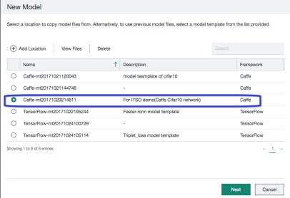
Figure 6-77 Creating a Cifar-10 model
2. Select this model template, and click Next. The Add Caffe model window opens. Table 6-8 shows the parameters to be entered in this window.
Table 6-8 List of parameters and values for the template model
|
Parameter
|
Value
|
|
Create an inference model
|
unmark
|
|
Model name
|
Cifar10-ITSO-Demo-1
|
|
Model description
|
For ITSO demonstration (Caffe Cifar-10 network)
|
|
Training engine
|
Native
|
|
Training data set
|
Cifar10-testdata
|
|
Base learning rate
|
0.01 (Default)
|
|
Momentum
|
0.9 (Default)
|
|
Weight decay
|
0.0004 (Default)
|
|
Max Iterations
|
40000 (Default)
|
|
Optimizer type
|
Stochastic gradient descent (SGD) (Default)
|
|
Learning rate policy
|
Fix (Default)
|
|
Batch size
|
96
|
|
Note: For the first parameter, because you are creating a model for training, unmask it. If you want to create a model for inference, select it.
For the training engine type choices, there are Single, Native, Fabric, and Elastic.
For the hyperparameters, you can change them based on your experiences.
|
3. Click Add to complete model creation. A new item is added to the Models list. Select it and click Edit. Then, you can modify the configuration and prototxt files, as shown in Figure 6-78.

Figure 6-78 Editing the Cifar-10 network files
6.8.4 Model training
After the model is created, you can start a training task by completing the following steps:
1. Select the model and click Train. The Train Cifar10-ITSO-demo window opens. Table 6-9 shows the parameters that are used for the training task.
Table 6-9 Parameters for a training job
|
Parameter
|
Value
|
|
Name of the trained model
|
Cifar10-ITSO-demo1-20171030112822 (Default, can change)
|
|
Data set
|
cifar10-testdata-1
|
|
Number of workers
|
1
|
|
GPUs per worker
|
1
|
|
Framework
|
Caffe on Spark
|
|
Weight files on the remote server
|
See note below.
|
|
Note: In this environment, we have only one node, which has one GPU, so the Number of workers and GPUs per worker should be 1.
For the last parameter, there is one weight file that we want to use to continue training for this scenario. You can fill in the path for the weight file that you want to use.
|
2. Click Start training, and the training task starts. To monitor the process of this training job, open the MAO window. Click the current training model Cifar10-ITSO-demo, click Training, select one training task, and click Insights. The MAO window is shown in Figure 6-79.

Figure 6-79 Monitoring and Optimization window for this training model
3. Figure 6-79 shows a suggestion for this training job. Click Optimize at the upper right of the loss graph. Figure 6-80 shows the optimization suggestion for this training job.

Figure 6-80 Optimization suggestion for this training job
4. Use this new learning rate value (Figure 6-80 on page 219) to start another training job, and get the result, as shown in Figure 6-81.

Figure 6-81 Monitoring and Optimization window for this training model
You can compare the accuracy of these two models by using the model validation function, which is described in 6.8.5, “Model validation” on page 220.
6.8.5 Model validation
To do model validation, complete the validation data set when you import the data set by completing the following steps:

Figure 6-82 Starting a validation job
2. Because this is an image classification scenario, select Top K and set the number to 1, as shown in Figure 6-83 on page 221.

Figure 6-83 Selecting the validation method
When the two validation jobs are complete, click Validation Results to get the result, as shown in Figure 6-84.

Figure 6-84 Checking the validation result
From the output that is shown in Figure 6-84, the accuracy of the original trained model is 69.28%. After you tune the learning rate from 0.01 to 0.005, the accuracy of the new trained model is 73.1%.
6.8.6 Model tuning
This section describes the DLI’s hyperparameter tuning function to tune the model. Complete the following steps:

Figure 6-85 Starting a hyperparameter tuning task
The Hyperparameter Tuning window opens. In this use case, we tune only the Weight decay to explain how DLI works. Table 6-10 shows the parameter configuration for this tuning task.
Table 6-10 Parameters for this model tuning task
|
Parameter
|
Value
|
|
Name of tuning attempt
|
Cifar10-ITSO-demo1-20171030120407
|
|
Hyperparameter search type
|
Random Search
|
|
Framework
|
CaffeOnSpark
|
|
Optimizer type
|
SGD
|
|
Learning rate range
|
0.005
|
|
Weight decay range
|
0.0004-0.004 (it was 0.0004 in previous models)
|
|
Momentum range
|
0.9
|
|
Max batch size
|
96
|
|
Number of workers
|
1
|
|
GPUs per worker
|
1
|
|
Max iterations
|
40000
|
|
Total tuning jobs number
|
10 (default)
|
|
Max tuning jobs in parallel
|
2 (default)
|
|
Max running time (minutes)
|
60 (default)
|
2. Click Start Tuning and wait for several minutes for this tuning task to complete. Select the tuning task and click the name. The window shows the tuning result, as shown in Figure 6-86.
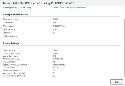
Figure 6-86 Viewing a tuning result
During this tuning task, DLI identifies the best Weight decay value as 0.0019329544. DLI created a training model with the tuned hyperparameters. Figure 6-87 shows the new item in the training model list.

Figure 6-87 Starting a train job base on the tuned model
3. Start a new training job with this model, as shown in the MAO dashboard in Figure 6-88.

Figure 6-88 Monitoring and Optimization window for this training model
4. Select this trained job (Figure 6-88) and click Validation Trained Model to trigger a validation job. The result is shown in Figure 6-89.

Figure 6-89 Viewing a validation result for the tuned model
The output shows that the accuracy is 75.21%, which means that with the DLI’s hyperparameter tuning’s help, the accuracy changed from 73.1% to 75.21%. Table 6-11 on page 225 shows the summary of accuracy for the different scenarios.
Table 6-11 Summary of accuracy result for different trained jobs
|
Scenario
|
Operation
|
Accuracy
|
|
Baseline
|
Not applicable
|
69.28%
|
|
DLI suggestion during training
|
Learning rate:
0.01 - 0.005
|
73.1%
|
|
DLI suggestion during hyperparameter search
|
Weight decay:
0.0004 - 0.0019329544
|
75.21%
|
|
Note: This is a straightforward example to demonstrate how to use DLI to tune a neural network model. In production cases, DLI can help you to keep to the correct tuning direction and get better accuracy.
|
6.8.7 Model prediction
When you are satisfied with the accuracy of one trained model, create an inference model for prediction by completing the following steps:

Figure 6-90 Generating an inference model
2. DLI creates a new inference model, and you can find it in the model list, as shown in Figure 6-91. Select this model and click Inference.

Figure 6-91 Starting an inference job
3. Complete the threshold and select the files on which you want to do prediction. Click Start Inference, as shown in Figure 6-92.
|
Note: If you set the threshold to 0.1, this means DLI displays all the classes with similar possibilities to >= 10%.
|

Figure 6-92 Setting the parameters for an inference job
4. When this inference job completes, DLI creates an inference result item in a reference list. Click the name and you can see the result, as shown in Figure 6-93 on page 227.

Figure 6-93 Selecting an inference job
Figure 6-94 shows the prediction result of the inference job.

Figure 6-94 Viewing the result of the inference job
Prediction through the RESTful API
You can also use the RESTful API to call the inference service. Example 6-17 shows how to implement it with a Python script and integrate the application to call the DL prediction service.
Example 6-17 Using a RESTful API to call the DLI inference service
import requests
from requests.packages.urllib3.exceptions import InsecureRequestWarning
requests.packages.urllib3.disable_warnings(InsecureRequestWarning)
import base64
import json
import time
import os
###Set variables, changed by real requirement###
lv_host='cwsdli01.dli.com'
lv_inference_model='Cifar10-ITSO-demo1-tuning-20171030120407-20171030142006-20171030143328-Inference'
lv_threshold=0.1
lv_img_dir='/demodata/userdata/cifar10_test/'
lv_user='Admin'
lv_passwd='Admin'
###Logon###
logonUrl='https://'+lv_host+':8643/platform/rest/conductor/v1/auth/logon'
base64string = base64.encodestring('%s:%s' % (lv_user, lv_passwd)).replace('
', '')
auth='Basic ' + base64string
headers = {'Authorization': auth}
req = requests.Session()
r = req.get(logonUrl, headers=headers, verify=False)
if 200 != r.status_code:
print('logon failed')
print('logon to rest server succeed')
###Get file list from directory###
files = {}
for idirpath, dirnames, filenames in os.walk(lv_img_dir, followlinks=True):
count = 0
for filep in filenames:
count += 1
tmp_file = os.path.join(lv_img_dir,filep)
files['file'+str(count)] = open(tmp_file,'rb')
print files
###Start a new inference task###
startInferenceUrl='https://' + lv_host + ':9243/platform/rest/deeplearning/v1/inferences/startpredict'
inf_name='Inference' + str(int(time.time()))
data={'predictname':inf_name, 'modelname':lv_inference_model,'threshold':lv_threshold}
r = req.post(startInferenceUrl,data=data, files=files,verify=False)
print('Start inference task: %s'%inf_name)
print('Waiting for Inference spark application lanuched...')
###Check inference task status###
getInferenceStatusUrl='https://' + lv_host + ':9243/platform/rest/deeplearning/v1/inferences/' + inf_name
getInferenceResUrl='https://' + lv_host + ':9243/platform/rest/deeplearning/v1/inferences/' + inf_name + '/predicts'
commonHeaders={'accept': 'application/json'}
r = req.get(getInferenceStatusUrl,headers=commonHeaders, verify=False)
json_out=r.json()
if json_out.has_key('status'):
while json_out['status'] != 'FINISHED':
print('Inference task current status: %s'%json_out['status'])
r = req.get(getInferenceStatusUrl,headers=commonHeaders, verify=False)
json_out=r.json()
###This task is finished and print output###
print('Inference task is FINISHED')
r = req.get(getInferenceResUrl,headers=commonHeaders, verify=False)
print('Here is the inference output:')
print(json.dumps(r.json(), sort_keys=True, indent=4))
else:
print('Failed to get Inference task status, exit')
Example 6-18 shows the output after running this script. The output can be used by your application directly.
Example 6-18 Output of the prediction script
#python cifar10_inference.py
logon to rest server succeed
{'file1': <open file '/demodata/userdata/cifar10_test/car_s.png', mode 'rb' at 0x3fffae6abf60>}
Start inference task: Inference1509378367
Waiting for Inference spark application lanuched...
...
Inference task is FINISHED
Here is the inference output:
{
"classificationResults": [
{
"image": true,
"inputPath": "/scratch/dli_userdata/models/Caffe/Cifar10-ITSO-demo1-tuning-20171030120407-20171030142006-20171030143328-Inference/Inference1509378367/inputs",
"results": [
{
"label": "automobile",
"prob": 0.757
}
],
"sampleId": "car_s.png"
}
],
"type": "classification"
}
6.8.8 Training model weight file management
When one training model job is complete, download its weight file. This weight file is used to deploy the inference model in any other server or use it for continuous training. Then, complete the following steps:

Figure 6-95 Downloading the weight file
2. A window opens and shows all the weight files. Click any of them to download, as shown in Figure 6-96.

Figure 6-96 Downloading a weight file
3. Transfer this file to another server, for example, upload it to /demodata/userdata/cifar10_weightfile, as shown in Figure 6-97.

Figure 6-97 Generating an inference model with one existing weight file

Figure 6-98 Viewing an inference model list and starting an inference job
This inference model can be used for prediction by using the GUI or the RESTful API.
..................Content has been hidden....................
You can't read the all page of ebook, please click here login for view all page.