

Testing the environment
In this chapter we provide information on how to establish test plans, test the different components of your environment at the operating system level, how to interpret information reported by the analysis tools, how to spot bottlenecks, and how to manage your workload. This information can be used by those who are either building a system from scratch, applying all the concepts from the previous chapters, or those who are looking for an improvement of a production environment.
We help you establish and implement tests of the environment, and give you some guidance to understand the results of the changes implemented.
The following topics are discussed in this chapter:
5.1 Understand your environment
Submitting an environment for performance analysis is often a complex task. It usually requires a good knowledge of the workloads running, system capacity, technologies available, and it involves a lot of tuning and tests.
To understand the limits of the different components of the environment is crucial to establish baselines and targets and set expectations.
5.1.1 Operating system consistency
While keeping AIX levels up to date is an obvious concern, keeping things consistent is often overlooked. One LPAR might have been updated with a given APAR or fix, but how to be sure it was also applied to other LPARs of the same levels? Not maintaining consistency is a way of introducing performance problems, as some LPARs can remain backlevel or unpatched. There are many ways to track levels of installed AIX across LPARs. One often overlooked option is provided by NIM.
The niminv command allows administrators to gather, conglomerate, compare and download fixes based on installation inventory of NIM objects. It provides an easy method to ensure systems are at an expected level.
niminv can use any NIM object that contains installation information. Examples include standalone client, SPOT, lpp_source and mksysb objects.
Using niminv has the following benefits:
•Hardware installation inventory is gathered alongside the software installation inventory.
•Data files are saved with a naming convention that is easily recognizable.
Example 5-1 illustrates using niminv to compare one NIM client (aix13) with another (aix19). For each NIM client there will be a column. The value will either be listed “same” if the level for the file set is the same for the target as the base, and “-” if missing and the actual level if existing but different (higher or lower).
Example 5-1 Using niminv with invcom to compare installed software levels on NIM clients
root@nim1: /usr/sbin/niminv -o invcmp -a targets=‘aix13,aix19' -a base=‘aix13' -a location='/tmp/123‘
Comparison of aix13 to aix13:aix19 saved to /tmp/123/comparison.aix13.aix13:aix19.120426230401.
Return Status = SUCCESS
root@nim1: cat /tmp/123/comparison.aix13.aix13:aix19.120426230401
# name base 1 2
----------------------------------------- ---------- ---------- ----------
AIX-rpm-7.1.0.1-1 7.1.0.1-1 same same
...lines omitted...
bos.64bit 7.1.0.1 same same
bos.acct 7.1.0.0 same same
bos.adt.base 7.1.0.0 same same
bos.adt.include 7.1.0.1 same same
bos.adt.lib 7.1.0.0 same same
...lines omitted...
bos.rte 7.1.0.1 same same
...lines omitted...
base = comparison base = aix13
1 = aix13
2 = aix19
'-' = name not in system or resource
same = name at same level in system or resource
5.1.2 Operating system tunable consistency
In environments where tunables beyond the defaults are required, it is important to maintain an overview of what is applied across an environment, and to ensure that tunables are consistent and not removed. Also, to keep track of what is applied as a reminder in case some only need to be temporarily enabled.
System tunable consistency check can be done using the AIX Runtime Expert (ARTEX). The existing samples in the /etc/security/artex/samples directory can be used to create a new profile with the artexget command, which can be customized. The corresponding catalog in /etc/security/artex/catalogs is referred to for retrieving and setting values for that parameter.
|
Note: The artexget and artexset commands execute the <GET> and <SET> sections, respectively, in the cfgMethod of the Catalog which is defined for a particular parameter.
|
Example 5-2 shows a simple profile, which can be used with ARTEX tools.
Example 5-2 AIX Runtime Expert sample profile
root@nim1: cat /etc/security/artex/samples/aixpertProfile.xml
<?xml version="1.0" encoding="UTF-8"?>
<Profile origin="reference" readOnly="true" version="2.0.0">
<Catalog id="aixpertParam" version="2.0">
<Parameter name="securitysetting"/>
</Catalog>
</Profile>
Example 5-3 shows a simple catalog that can be used with the ARTEX tools with a corresponding profile. Note the Get and Set stanzas and Command and Filter attributes, which can be modified and used to create customized catalogues to extend the capabilities of ARTEX.
Example 5-3 AIX Runtime Expert sample catalog
root@nim1: cat /etc/security/artex/catalogs/aixpertParam.xml
<?xml version="1.0" encoding="UTF-8"?>
<Catalog id="aixpertParam" version="2.0" priority="-1000">
<ShortDescription><NLSCatalog catalog="artexcat.cat" setNum="2" msgNum="1">System security level configuration.</NLSCatalog></ShortDescription>
<Description><NLSCatalog catalog="artexcat.cat" setNum="2" msgNum="2">The aixpert command sets a variety of system configuration settings to enable the desired security level.</NLSCatalog></Description>
<ParameterDef name="securitysetting" type="string">
<Get type="current">
<Command>/etc/security/aixpert/bin/chk_report</Command>
<Filter>tr -d '
'</Filter>
</Get>
<Get type="nextboot">
<Command>/etc/security/aixpert/bin/chk_report</Command>
<Filter>tr -d '
'</Filter>
</Get>
<Set type="permanent">
<Command>/usr/sbin/aixpert -l %a</Command>
<Argument>`case %v1 in 'HLS') echo 'h';; 'MLS') echo 'm';; 'LLS') echo 'l';; 'DLS') echo 'd';; 'SCBPS') echo 's';; *) echo 'd';; esac`</Argument>
</Set>
</ParameterDef>
</Catalog>
One method to employ these capabilities is to use NIM to perform an ARTEX operation on a group of systems (Example 5-4); this would provide a centralized solution to GET, SET and compare (DIFF) the attribute values across the group.
Example 5-4 Using NIM script to run AIX Runtime Expert commands on NIM clients
root@nim1: cat /export/scripts/artex_diff
root@nim1: artexget -r -f txt /etc/security/artex/samples/viosdevattrProfile.xml
root@nim1: nim -o define -t script -a server=master -a location=/export/scripts/artex_diff artex_diff
root@nim1: nim -o allocate -a script=artex_diff nimclient123
root@nim1: nim -o cust nimclient123
Component name Parameter name Parameter value Additional Action
----------------- ------------------- ----------------- -----------------------
viosdevattrParam reserve_policy no_reserve NEXTBOOT
viosdevattrParam queue_depth 3 NEXTBOOT
...lines omitted...
5.1.3 Size that matters
The world is dynamic. Everything changes all the time and businesses react in the same way. When you do performance analysis on the environment, you will eventually find that the problem is not how your systems are configured, but instead how they are sized. The initial sizing for a specific workload may not fit your business needs after a while. You may find out that some of your infrastructure is undersized or even oversized for different workloads and you have to be prepared to change.
5.1.4 Application requirements
Different applications are built for different workloads. An application server built for a demand of ten thousand users per month may not be ready to serve one hundred thousand users. This is a typical scenario where no matter how you change your infrastructure environment, you do not see real benefits of the changes you have made unless your application is also submitted to analysis.
5.1.5 Different workloads require different analysis
One of the most important factors when you analyze your systems is that you have a good understanding of the different types of workloads that you are running. Having that knowledge will lead you to more objective work and concise results.
5.1.6 Tests are valuable
Each individual infrastructure component has its own limitations, and understanding these different limits is never easy. For example, similar network adapters show different throughputs depending on other infrastructure components like the number of switches, routers, firewalls, and their different configurations. Storage components are not different, they behave differently depending on different factors.
•Individual tests
A good way to understand the infrastructure limits is by testing the components individually so that you know what to expect from each of them.
•Integration tests
Integration tests are good to get an idea about how the infrastructures interact and how that affects the overall throughput.
|
Note: Testing your network by transmitting packets between two ends separated by a complex infrastructure, for example, can tell you some data about your environment throughput but may not tell you much about your individual network components.
|
5.2 Testing the environment
This section offers some suggestions on how to proceed with testing your environment. By doing so systematically you should be able to determine whether the changes made based on the concepts presented throughout this book have beneficial results on your environment.
A good thing to keep in mind is that not every system or workload will benefit from the same tuning.
5.2.1 Planning the tests
When the environment is going to be tested, it is good practice to establish goals and build a test plan.
The following topics are important things to be considered when building a test plan:
•Infrastructure
Knowledge about the type of machines, their capacity, how they are configured, partition sizing, resource allocation, and about other infrastructure components (network, storage) is important. Without this information it is just hard to establish baselines and goals, and to set expectations.
•Component tests
Test one component at a time. Even though during the tests some results may suggest that other components should be tuned, testing multiple components may not be a good idea since it involves a lot of variables and may lead to confusing results.
•Correct workload
The type of workload matters. Different workloads will have different impact on the tests, and thus it is good to tie the proper workload to the component being tested as much as possible.
•Impact and risk analysis
Tests may stress several components at different levels. The impact analysis of the test plan should consider as many levels as possible to mitigate any major problems with the environment.
In the past years, with all the advance of virtualized environments, shared resources have become a new concern when testing. Stressing a system during a processor test may result in undesired resource allocations. Stressing the disk subsystem might create bottlenecks for other production servers.
•Baselines and goals
Establishing a baseline is not always easy. The current environment configuration has to be evaluated and monitored before going through tests and tuning. Without a baseline, you have nothing to compare with your results.
Defining the goals you want to achieve depends on understanding of the environment. Before establishing a performance gain on network throughput of 20%, for instance, you must first know how the entire environment is configured.
Once you have a good understanding of how your environment behaves and its limitations, try establishing goals and defining what is a good gain, or what is a satisfactory improvement.
•Setting the expectations
Do not assume that a big boost in performance can always be obtained. Eventually you may realize that you are already getting the most out of your environment and further improvements can only be obtained with new hardware or with better-written applications.
Be reasonable and set expectations of what is a good result for the tests.
Expectations can be met, exceeded, or not met. In any case, tests should be considered an investment. They can give you a good picture of how the environment is sized, its ability to accommodate additional workload, estimation of future hardware needs, and the limits of the systems.
5.2.2 The testing cycle
A good approach to test the environment is to establish cycles of tests, broken into the following steps:
•Establish a plan
Set the scope of your tests, which components will be tested, which workloads will be applied, whether they are real or simulation, when tests will be made, how often the system will be monitored, and so on.
•Make the changes
Change the environment according to the plan, trying to stay as much as possible inside the scope of the defined plan.
•Monitor the components
Establish a period to monitor the system and collect performance data for analysis. There is no best period of time for this, but usually a good idea is to monitor the behavior of the system for a few days at least and try to identify patterns.
•Compare the results
Compare the performance data collected with the previous results. Analysis of the results can be used as an input to a new cycle of tests with a new baseline.
You can establish different plans, test each one in different cycles, measure and compare the results, always aiming for additional improvement. The cycle can be repeated as many times as necessary.
5.2.3 Start and end of tests
This section provides information on when to start and end the tests.
When to start testing the environment
A good time to start profiling the environment is now. Unless you have a completely static environment, well sized and stable, tests should be a constant exercise.
Workload demands tend to vary either by increasing or decreasing with time, and analyzing the environment is a good way to find the right moment to review the resource distribution.
Imagine a legacy system being migrated to a new environment. The natural behavior is for a new system to demand more resources with time, and the legacy system demanding less.
When to stop testing the environment
Testing the environment takes time, requires resources, and has costs. At some point, tests will be interrupted by such restrictions.
Despite these restrictions, assuming that a plan has been established at the beginning, the best moment to stop the tests is when the results achieve at least some of the established goals.
The reasons why an environment is submitted to tests can vary and no matter what the goals of the tests are, their results should be meaningful and in accordance with the goals defined, even if you cannot complete all the tests initially planned.
Systems have limits
Every environment has its limits but only tests will tell what your environment’s are. Eventually you may find that even though everything has been done on the system side, the performance of the applications is still not good. You may then want to take a look at the application architecture.
5.3 Testing components
In this section we try to focus on simple tests of the components, and which tools you can use to monitor system behavior, to later demonstrate how to read and interpret the measured values.
Testing the system components is usually a simple task and can be accomplished by using native tools available on the operating system by writing a few scripts. For instance, you may not be able to simulate a multithread workload with the native tools, but you can spawn a few processor-intensive processes and have an idea of how your system behaves.
Basic network and storage tests are also easy to perform.
|
Note: It is not our intention to demonstrate or compare the behavior of processes and threads. The intention of this section is to put a load on the processor of our environment and use the tools to analyze the system behavior.
|
How can I know, for example, that the 100 MB file retrieval response time is reasonable? Its response time is composed of network transmission + disk reading + application overhead. I should be able to calculate that, in theory.
5.3.1 Testing the processor
Before testing the processing power of the system, it is important to understand the concepts explained in this book because there are a lot of factors that affect the processor utilization of the system.
To test the processor effectively, the ideal is to run a processor-intensive workload. Running complex systems that depend on components such as disk storage or networks might not result in an accurate test of the environment and can result in misleading data.
The process queue
The process queue is a combination of two different queues: the run queue and wait queue. Threads on the run queue represent either threads ready to run (awaiting for a processor time slice) or threads already running. The wait queue holds threads waiting for resources or I/O requests to complete.
Running workloads with a high number of processes is good for understanding the response of the system and to try to establish the point at which the system starts to become unresponsive.
In this section, the nstress suite has been used to put some load on the system. The tests are made running the ncpu command starting with 16 processes. On another window we monitored the process queue with the vmstat command, and a one-line script to add time information at the front of each line to check the output. Table 5-1 illustrates the results.
Table 5-1 Tests run on the system
|
Processes
|
System response
|
|
16
|
Normal
|
|
32
|
Normal
|
|
64
|
Minimal timing delays
|
|
96
|
Low response. Terminals not responding to input.
|
|
128
|
Loss of output from vmstat.
|
The system performed well until we put almost a hundred processes on the queue. Then the system started to show slow response and loss of output from vmstat, indicating that the system was stressed.
A different behavior is shown in Example 5-5. In this test, we started a couple of commands to create one big file and several smaller files. The system has only a few processes on the run queue, but this time it also has some on the wait queue, which means that the system is waiting for I/O requests to complete. Notice that the processor is not overloaded, but there are processes that will keep waiting on the queue until their I/O operations are completed.
Example 5-5 vmstat output illustrating processor wait time
vmstat 5
System configuration: lcpu=16 mem=8192MB ent=1.00
kthr memory page faults cpu
----- ----------- ------------------------ ------------ -----------------------
r b avm fre re pi po fr sr cy in sy cs us sy id wa pc ec
2 1 409300 5650 0 0 0 23800 23800 0 348 515 1071 0 21 75 4 0.33 33.1
1 3 409300 5761 0 0 0 23152 75580 0 340 288 1030 0 24 67 9 0.37 36.9
3 4 409300 5634 0 0 0 24076 24076 0 351 517 1054 0 21 66 12 0.34 33.8
2 3 409300 5680 0 0 0 24866 27357 0 353 236 1050 0 22 67 11 0.35 34.8
0 4 409300 5628 0 0 0 22613 22613 0 336 500 1036 0 21 67 12 0.33 33.3
0 4 409300 5622 0 0 0 23091 23092 0 338 223 1030 0 21 67 12 0.33 33.3
5.3.2 Testing the memory
This topic addresses some tests that can be made at the operating system level to measure how much workload your current configuration can take before the system becomes unresponsive or kills processes.
The system we were using for the tests was a partition with 8 GB of RAM and 512 Mb of paging-space running AIX 7.1. To simulate the workload, we used the stress tool, publicly available under GPLv2 license at:
http://weather.ou.edu/~apw/projects/stress/
Packages ready for the AIX can be found at:
http://www.perzl.org/aix
The following tests were intended to test how much memory load our system could take before starting to swap, become unresponsive, and kill processes.
The first set of tests tried to establish how many processes we could dispatch using different memory sizes. Before starting the tests, it is important to have a good understanding of virtual memory concepts and how the AIX Virtual Memory Manager works.
There are a few tunables that will affect the behavior of our system during the tests.
The npswarn, npskill, and nokilluid tunables
When AIX detects that memory resource is running out, it might kill processes to release a number of paging space pages to continue running. AIX controls this behavior through the npswarn, npskill and nokilluid tunables.
•npswarn
The npswarn tunable is a value that defines the minimum number of free paging space pages that must be available. When this threshold is exceeded, AIX will start sending the SIGDANGER signal to all processes except kernel processes.
The default action for SIGDANGER is to ignore this signal. Most processes will ignore this signal. However, the init process does register a signal handler for the SIGDANGER signal, which will write the warning message Paging space low to the defined system console.
The kernel processes can be shown using ps -k. Refer to the following website for more information about kernel processes (kprocs):
•npskill
If consumption continues, this tunable is the next threshold to trigger; it defines the minimum number of free paging-space pages to be available before the system starts killing processes.
At this point, AIX will send SIGKILL to eligible processes depending on the following factors:
– Whether or not the process has a SIGDANGER handler
By default, SIGKILL will only be sent to processes that do not have a handler for SIGDANGER. This default behavior is controlled by the vmo option low_ps_handling.
– The value of the nokilluid setting, and the UID of the process, which is discussed in the following section.
– The age of the process
AIX will first send SIGKILL to the youngest eligible process. This helps to prevent long running processes against a low paging space condition caused by recently created processes. Now you understand why you cannot establish telnet or ssh connections to the system, but still ping it at this point?
However, note that the long running processes could also be killed if the low paging space condition (below npskill) persists.
When a process is killed, the system logs a message with the label PGSP_KILL, as shown in Example 5-6.
Example 5-6 errpt output - Process killed by AIX due to lack of paging space
LABEL: PGSP_KILL
IDENTIFIER: C5C09FFA
Date/Time: Thu Oct 25 12:49:32 2012
Sequence Number: 373
Machine Id: 00F660114C00
Node Id: p750s1aix5
Class: S
Type: PERM
WPAR: Global
Resource Name: SYSVMM
Description
SOFTWARE PROGRAM ABNORMALLY TERMINATED
Probable Causes
SYSTEM RUNNING OUT OF PAGING SPACE
Failure Causes
INSUFFICIENT PAGING SPACE DEFINED FOR THE SYSTEM
PROGRAM USING EXCESSIVE AMOUNT OF PAGING SPACE
Recommended Actions
DEFINE ADDITIONAL PAGING SPACE
REDUCE PAGING SPACE REQUIREMENTS OF PROGRAM(S)
Detail Data
PROGRAM
stress
USER'S PROCESS ID:
5112028
PROGRAM'S PAGING SPACE USE IN 1KB BLOCKS
8
The error message gives the usual information with timestamp, causes, recommended actions and details of the process.
In the example, the process stress has been killed. For the sake of our tests, it is indeed the guilty process for inducing shortages on the system. However, in a production environment the process killed is not always the one that is causing the problems. Whenever this type of situation is detected on the system, a careful analysis of all processes running on the system must be done during a longer period. The nmon tool is a good resource to assist with collecting data to identify the root causes.
In our tests, when the system was overloaded and short on resources, AIX would sometimes kill our SSH sessions and even the SSH daemon.
|
Tip: The default value for this tunable is calculated with the formula:
npskill = maximum(64, number_of_paging_space_pages/128)
|
•nokilluid
This tunable accepts a UID as a value. All processes owned by UIDs below the defined value will be out of the killing list. Its default value is zero (0), which means that even processes owned by the root ID can be killed.
Now that we have some information about these tunables, it is time to proceed with the tests.
One major mistake that people make is to think that a system with certain amounts of memory can take a load matching that same size. This viewpoint is incorrect; if your system has 16 GB of memory, it does not mean that all the memory can be made available to your applications. There are several other processes and kernel structures that also need memory to work.
In Example 5-7, we illustrate the wrong assumption by adding a load of 64 processes, with 128 MB of size each to push the system to its limits (64 x 128 = 8192). The expected result is an overload of the virtual memory and a reaction from the operating system.
Example 5-7 stress - 64x 128MB
# date ; stress -m 64 --vm-bytes 128M -t 120 ; date
Thu Oct 25 15:22:15 EDT 2012
stress: info: [15466538] dispatching hogs: 0 cpu, 0 io, 64 vm, 0 hdd
stress: FAIL: [15466538] (415) <-- worker 4259916 got signal 9
stress: WARN: [15466538] (417) now reaping child worker processes
stress: FAIL: [15466538] (451) failed run completed in 46s
Thu Oct 25 15:23:01 EDT 2012
As seen in bold, the process receives a SIGKILL less than a minute after being started. The reason is that the resource consumption levels reached the limits defined by the npswarn and npskill parameters. This is illustrated in Example 5-8. At 15:22:52 (time is in the last column), the system is exhausted of free memory pages and showing some paging space activity. At the last line, the system had a sudden increase on the paging out and replacement, indicating that the operating system had to make some space by freeing some pages to accommodate the new allocation.
Example 5-8 vmstat output - 64 x 128 MB
# vmstat -t 1
System configuration: lcpu=16 mem=8192MB ent=1.00
kthr memory page faults cpu time
----- ----------- ------------------------- ------------ ----------------------- --------
r b avm fre re pi po fr sr cy in sy cs us sy id wa pc ec hr mi se
67 0 1128383 1012994 0 1 0 0 0 0 9 308 972 99 1 0 0 3.82 381.7 15:22:19
65 0 1215628 925753 0 0 0 0 0 0 2 50 1104 99 1 0 0 4.01 400.7 15:22:20
65 0 1300578 840779 0 0 0 0 0 0 10 254 1193 99 1 0 0 3.98 398.2 15:22:21
65 0 1370827 770545 0 0 0 0 0 0 11 54 1252 99 1 0 0 4.00 400.2 15:22:22
64 0 1437708 703670 0 0 0 0 0 0 20 253 1304 99 1 0 0 4.00 400.0 15:22:23
66 0 1484382 656996 0 0 0 0 0 0 11 50 1400 99 1 0 0 4.00 399.6 15:22:24
64 0 1554880 586495 0 0 0 0 0 0 12 279 1481 99 1 0 0 3.99 398.9 15:22:25
64 0 1617443 523931 0 0 0 0 0 0 4 47 1531 99 1 0 0 3.99 398.7 15:22:26
...
38 36 2209482 4526 0 383 770 0 54608 0 467 138 1995 85 15 0 0 3.99 398.7 15:22:52
37 36 2209482 4160 0 364 0 0 62175 0 317 322 1821 87 13 0 0 3.99 399.5 15:22:53
33 40 2209482 4160 0 0 0 0 64164 0 7 107 1409 88 12 0 0 4.00 399.7 15:22:54
34 42 2209544 4173 0 49 127 997 50978 0 91 328 1676 87 13 0 0 4.01 400.8 15:22:55
31 48 2211740 4508 0 52 2563 3403 27556 0 684 147 2332 87 13 0 0 3.98 398.5 15:22:56
Killed
This is normal behavior and indicates that the system is very low on resources (based on VMM tunable values). In sequence, the system would just kill the vmstat process along with other application processes in an attempt to free more resources.
Example 5-9 has the svmon output for a similar example (the header has been added manually to make it easier to identify the columns). This system has 512 MB of paging space, divided into 131072 x 4096 KB pages. The npswarn and npskill values are 4096 and 1024, respectively.
Example 5-9 svmon - system running out of paging space
# svmon -G -i 5 | egrep "^(s)"
PageSize PoolSize inuse pgsp pin virtual
s 4 KB - 188996 48955 179714 229005
s 4 KB - 189057 48955 179725 229066
s 4 KB - 442293 50306 181663 482303
s 4 KB - 942678 51280 182637 982682
s 4 KB - 1222664 51825 183184 1262663
s 4 KB - 1445145 52253 183612 1485143
s 4 KB - 1660541 52665 184032 1700504
s 4 KB - 1789863 52916 184283 1829823
s 4 KB - 1846800 53196 184395 1887575
s 4 KB - 1846793 78330 184442 1912289
s 4 KB - 1846766 85789 184462 1921204
s 4 KB - 1846800 94455 184477 1929270
s 4 KB - 1846800 110796 184513 1948082
s 4 KB - 1846800 128755 184543 1963861
s 4 KB - 185921 49540 179756 229097
s 4 KB - 185938 49536 179756 229097
Subtracting the number of paging-space pages allocated from the total number of paging spaces, the number of free paging-space frames will be:
131072 - 128755 = 2317 (free paging-space frames)
The resulting value is between npswarn and npskill. Thus, at that specific moment, the system was about to start killing processes and the last two lines of Example 5-9 on page 218 show a sudden drop of the paging-space utilization indicating that some processes have terminated (in this case they were killed by AIX).
The last example illustrated the behavior of the system when we submitted a load of processes matching the size of the system memory. Now, let us see what happens when we use bigger processes (1024 MB each), but with a fewer number of processes (7).
The first thing to notice in Example 5-10 is that the main process got killed by AIX.
Example 5-10 stress output - 7x1024 MB processes
# stress -m 7 --vm-bytes 1024M -t 300
stress: info: [6553712] dispatching hogs: 0 cpu, 0 io, 7 vm, 0 hdd
Killed
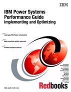
Although our main process got killed, we still had six processes running, each 1024 MB in size, as shown in Example 5-11, which also illustrates the memory and paging space consumption.
Example 5-11 topas output - 7x1024 MB processes
Topas Monitor for host:p750s1aix5 EVENTS/QUEUES FILE/TTY
Tue Oct 30 15:38:17 2012 Interval:2 Cswitch 226 Readch 1617
Syscall 184 Writech 1825
CPU User% Kern% Wait% Idle% Physc Entc% Reads 9 Rawin 0
Total 76.7 1.4 0.0 21.9 4.00 399.72 Writes 18 Ttyout 739
Forks 0 Igets 0
Network BPS I-Pkts O-Pkts B-In B-Out Execs 0 Namei 0
Total 2.07K 11.49 8.50 566.7 1.52K Runqueue 7.00 Dirblk 0
Waitqueue 0.0
Disk Busy% BPS TPS B-Read B-Writ MEMORY
Total 0.5 56.0K 13.99 56.0K 0 PAGING Real,MB 8192
Faults 5636 % Comp 94
FileSystem BPS TPS B-Read B-Writ Steals 0 % Noncomp 0
Total 1.58K 9.00 1.58K 0 PgspIn 13 % Client 0
PgspOut 0
Name PID CPU% PgSp Owner PageIn 13 PAGING SPACE
stress 11927714 15.0 1.00G root PageOut 0 Size,MB 512
stress 13893870 14.9 1.00G root Sios 13 % Used 99
stress 5898362 12.5 1.00G root % Free 1
stress 9109570 12.2 1.00G root NFS (calls/sec)
stress 11206792 11.1 1.00G root SerV2 0 WPAR Activ 0
stress 12976324 10.9 1.00G root CliV2 0 WPAR Total 2
svmon 13959288 0.4 1.13M root SerV3 0 Press: "h"-help
sshd 4325548 0.2 1.05M root CliV3 0 "q"-quit
In Example 5-12, the svmon output illustrates the virtual memory. Even though the system still shows some free pages, it is almost out of paging space. During this situation, dispatching a new command could result in a fork() error.
Example 5-12 svmon - 7x 1024MB processes
size inuse free pin virtual mmode
memory 2097152 1988288 108864 372047 2040133 Ded
pg space 131072 130056
work pers clnt other
pin 236543 0 0 135504
in use 1987398 0 890
PageSize PoolSize inuse pgsp pin virtual
s 4 KB - 1760688 130056 183295 1812533
m 64 KB - 14225 0 11797 14225
Figure 5-1 illustrates a slow increase in memory pages consumption during the execution of six processes with 1024 MB each. We had almost a linear increase for a few seconds until the resources were exhausted and the operating system killed some processes.
The same tests running with memory sizes lower than 1024 MB would keep the system stable.

Figure 5-1 Memory pages slow increase
This very same test, running with 1048 MB processes for example, resulted in a stable system, with very low variation in memory page consumption.
These tests are all intended to understand how much load the server could take. Once the limits were understood, the application could be configured according to its requirements, behavior, and system limits.
5.3.3 Testing disk storage
When testing the attachment of an IBM Power System to an external disk storage system, and the actual disk subsystem itself, there are some important considerations before performing any meaningful testing.
Understanding your workload is a common theme throughout this book, and this is true when performing meaningful testing. The first thing is to understand the type of workload you want to simulate and how you are going to simulate it.
There are types of I/O workload characteristics that apply to different applications (Table 5-2).
Table 5-2 I/O workload types
|
I/O type
|
Description
|
|
Sequential
|
Sequential access to disk storage is where typically large I/O requests are sent from the server, where data is read in order, one block at a time one after the other. An example of this type of workload is performing a backup.
|
|
Random
|
Random access to disk storage is where data is read in random order from disk storage, typically in smaller blocks, and it is sensitive to latency.
|
An OLTP transaction processing-based workload typically will have a smaller random I/O request size between 4 k and 8 k. A data warehouse or batch type workload will typically have a larger sequential I/O request size of 16 k and larger. Again, a workload such as a backup server may have a sequential I/O block size of 64 k or greater.
Having a repeatable workload is key to be able to perform a test, make an analysis of the results, perform any attribute changes, and repeat the test. Ideally if you can perform an application-driven load test simulating the actual workload, this is going to be the most accurate method.
There are going to be instances where performing some kind of stress test without any application-driven load is going to be required. This can be performed with the ndisk64 utility, which requires minimal setup time and is available on IBM developerworks at:
|
Important: When running the ndisk64 utility against a raw device (such as an hdisk) or an existing file, the data on the device or file will be destroyed.
|
It is imperative to have an understanding of what the I/O requirement of the workload will be, and the performance capability of attached SAN and storage systems. Using SAP as an example, the requirement could be 35,000 SAPS, which equates to a maximum of 14,500 16 K random IOPS on a storage system with a 70:30 read/write ratio (these values are taken from the IBM Storage Sizing Recommendation for SAP V9).
Before running the ndisk64 tool, you need to understand the following:
•What type of workload are you trying to simulate? Random type I/O or sequential type I/O?
•What is the I/O request size you are trying to simulate?
•What is the read/write ratio of the workload?
•How long will you run the test? Will any production systems be affected during the running of the test?
•What is the capability of your SAN and storage system? Is it capable of handling the workload you are trying to simulate? We found that the ndisk64 tool was cache intensive on our storage system.
Example 5-13 demonstrates running the ndisk64 tool for a period of 5 minutes with our SAP workload characteristics on a test logical volume called ndisk_lv.
Example 5-13 Running the ndisk64 tool
root@aix1:/tmp # ./ndisk64 -R -t 300 -f /dev/ndisk_lv -M 20 -b 16KB -s 100G -r 70%
Command: ./ndisk64 -R -t 300 -f /dev/ndisk_lv -M 20 -b 16KB -s 100G -r 70%
Synchronous Disk test (regular read/write)
No. of processes = 20
I/O type = Random
Block size = 16384
Read-WriteRatio: 70:30 = read mostly
Sync type: none = just close the file
Number of files = 1
File size = 107374182400 bytes = 104857600 KB = 102400 MB
Run time = 300 seconds
Snooze % = 0 percent
----> Running test with block Size=16384 (16KB) ....................
Proc - <-----Disk IO----> | <-----Throughput------> RunTime
Num - TOTAL IO/sec | MB/sec KB/sec Seconds
1 - 136965 456.6 | 7.13 7304.84 300.00
2 - 136380 454.6 | 7.10 7273.65 300.00
3 - 136951 456.5 | 7.13 7304.08 300.00
4 - 136753 455.8 | 7.12 7293.52 300.00
5 - 136350 454.5 | 7.10 7272.05 300.00
6 - 135849 452.8 | 7.08 7245.31 300.00
7 - 135895 453.0 | 7.08 7247.49 300.01
8 - 136671 455.6 | 7.12 7289.19 300.00
9 - 135542 451.8 | 7.06 7228.26 300.03
10 - 136863 456.2 | 7.13 7299.38 300.00
11 - 137152 457.2 | 7.14 7314.78 300.00
12 - 135873 452.9 | 7.08 7246.57 300.00
13 - 135843 452.8 | 7.08 7244.94 300.00
14 - 136860 456.2 | 7.13 7299.19 300.00
15 - 136223 454.1 | 7.10 7265.29 300.00
16 - 135869 452.9 | 7.08 7246.39 300.00
17 - 136451 454.8 | 7.11 7277.23 300.01
18 - 136747 455.8 | 7.12 7293.08 300.00
19 - 136616 455.4 | 7.12 7286.20 300.00
20 - 136844 456.2 | 7.13 7298.40 300.00
TOTALS 2728697 9095.6 | 142.12 Rand procs= 20 read= 70% bs= 16KB
root@aix1:/tmp #
Once the ndisk testing has been completed, if it is possible to check the storage system to compare the results, and knowing the workload you generated was similar to the workload on the storage, it is useful to validate the test results.
Figure 5-2 shows the statistics displayed on our storage system, which in this case is an IBM Storwize V7000 storage system.
Figure 5-2 V7000 volume statistics
|
Note: 5.6, “Disk storage bottleneck identification” on page 251 describes how to interpret the performance data collected during testing activities.
|
It is also important to recognize that disk storage technology is evolving. With the introduction of solid state drives (SSD), new technologies have been adopted by most storage vendors, such as automated tiering. An example of this is the Easy Tier® technology used in IBM storage products such as IBM SAN Volume Controller, IBM DS8000 and IBM Storwize V7000.
Automated tiering monitors a workload over a period of time, and moves blocks of data in and out of SSD based on how frequently accessed they are. For example, if you run a test for 48 hours, and during that time the automated tiering starts moving blocks into SSD, the test results may vary. So it is important to consult your storage administrator on the storage system’s capabilities as part of the testing process.
5.3.4 Testing the network
Performing network tests on the environment is simpler than the other tests. From the operating system point of view, there is not much to be tested. Although some tuning can be performed on both AIX and Virtual I/O Server layers, for example, the information to be analyzed is more simple. However, when talking about networks, you should always consider all the infrastructure that may affect the final performance of the environment. Eventually you may find that the systems themselves are OK but some other network component, such as a switch, firewall, or router, is affecting the performance of the network.
Latency
Latency can be defined as the time taken to transmit a packet between two points. For the sake of tests, you can also define latency as the time taken for a packet to be transmitted and received between two points (round trip).
Testing the latency is quite simple. In the next examples, we used tools such as tcpdump and ping to test the latency of our infrastructure, and a shell script to filter data and calculate the mean latency (Example 5-14).
Example 5-14 latency.sh - script to calculate the mean network latency
#!/usr/bin/ksh
IFACE=en0
ADDR=10.52.78.9
FILE=/tmp/tcpdump.icmp.${IFACE}.tmp
# number of ICMP echo-request packets to send
PING_COUNT=10
# interval between each echo-request
PING_INTERVAL=10
# ICMP echo-request packet size
PING_SIZE=1
# do not change this. number of packets to be monitored by tcpdump before
# exitting. always PING_COUNT x 2
TCPDUMP_COUNT=$(expr "${PING_COUNT}*2")
tcpdump -l -i ${IFACE} -c ${TCPDUMP_COUNT} "host ${ADDR} and (icmp[icmptype] == icmp-echo or icmp[icmptype] == icmp-echoreply)" > ${FILE} 2>&1 &
ping -c ${PING_COUNT} -i ${PING_INTERVAL} -s ${PING_SIZE} ${ADDR} 2>&1
MEANTIME=$(cat ${FILE} | awk -F "[. ]" 'BEGIN { printf("scale=2;("); } { if(/ICMP echo request/) { REQ=$2; getline; REP=$2; printf("(%d-%d)+", REP, REQ); } } END { printf("0)/1000/10
"); }' | bc)
echo "Latency is ${MEANTIME}ms"
The script in Example 5-14 has a few parameters that can be changed to test the latency. This script can be changed to accept some command line arguments instead of having to change it every time.
Basically the script monitors the ICMP echo-request and echo-reply traffic while performing some ping with small packet sizes, and calculate the mean round-trip time from a set of samples.
Example 5-15 latency.sh - script output
# ksh latency.sh
PING 10.52.78.9 (10.52.78.9): 4 data bytes
12 bytes from 10.52.78.9: icmp_seq=0 ttl=255
12 bytes from 10.52.78.9: icmp_seq=1 ttl=255
12 bytes from 10.52.78.9: icmp_seq=2 ttl=255
12 bytes from 10.52.78.9: icmp_seq=3 ttl=255
12 bytes from 10.52.78.9: icmp_seq=4 ttl=255
12 bytes from 10.52.78.9: icmp_seq=5 ttl=255
12 bytes from 10.52.78.9: icmp_seq=6 ttl=255
12 bytes from 10.52.78.9: icmp_seq=7 ttl=255
12 bytes from 10.52.78.9: icmp_seq=8 ttl=255
12 bytes from 10.52.78.9: icmp_seq=9 ttl=255
--- 10.52.78.9 ping statistics ---
10 packets transmitted, 10 packets received, 0% packet loss
Latency is .13ms
Example 5-15 on page 224 shows the output of the latency.sh script containing the mean latency time of 0.13 ms. This test has been run between two servers connected on the same subnet sharing the same Virtual I/O server.
In Example 5-16, we used the tcpdump output to calculate the latency. The script filters each pair of requests and reply packets, extracts the timing portion required to calculate each packet latency, and finally sums all latencies and divides by the number of packets transmitted to get the mean latency.
Example 5-16 latency.sh - tcpdump information
# cat tcpdump.icmp.en0.tmp
tcpdump: verbose output suppressed, use -v or -vv for full protocol decode
listening on en0, link-type 1, capture size 96 bytes
15:18:13.994500 IP p750s1aix5 > nimres1: ICMP echo request, id 46, seq 1, length 12
15:18:13.994749 IP nimres1 > p750s1aix5: ICMP echo reply, id 46, seq 1, length 12
15:18:23.994590 IP p750s1aix5 > nimres1: ICMP echo request, id 46, seq 2, length 12
15:18:23.994896 IP nimres1 > p750s1aix5: ICMP echo reply, id 46, seq 2, length 12
15:18:33.994672 IP p750s1aix5 > nimres1: ICMP echo request, id 46, seq 3, length 12
15:18:33.994918 IP nimres1 > p750s1aix5: ICMP echo reply, id 46, seq 3, length 12
15:18:43.994763 IP p750s1aix5 > nimres1: ICMP echo request, id 46, seq 4, length 12
15:18:43.995063 IP nimres1 > p750s1aix5: ICMP echo reply, id 46, seq 4, length 12
15:18:53.994853 IP p750s1aix5 > nimres1: ICMP echo request, id 46, seq 5, length 12
15:18:53.995092 IP nimres1 > p750s1aix5: ICMP echo reply, id 46, seq 5, length 12
7508 packets received by filter
0 packets dropped by kernel
Latency times depend mostly on the network infrastructure complexity. This information can be useful if you are preparing the environment for applications that transmit a lot of small packets and demand low network latency.
Transmission tests - TCP_RR
Request and Response tests measure the number of transactions (basic connect and disconnect) that your servers and network infrastructure are able to handle. These tests were performed with the netperf tool (Example 5-17).
Example 5-17 netperf - TCP_RR test
# ./netperf -t TCP_RR -H 10.52.78.47
Netperf version 5.3.7.5 Jul 23 2009 16:57:35
TCP REQUEST/RESPONSE TEST: 10.52.78.47
(+/-5.0% with 99% confidence) - Version: 5.3.7.5 Jul 23 2009 16:57:41
Local /Remote ----------------
Socket Size Request Resp. Elapsed Response Time
Send Recv Size Size Time (iter) ------- --------
bytes Bytes bytes bytes secs. TRs/sec millisec*host
262088 262088 100 200 4.00(03) 3646.77 0.27
262088 262088
Transmission tests - TCP_STREAM
These tests attempt to send the most data possible from one side to another in a certain period and give the total throughput of the network. These tests were performed with the netperf tool (Example 5-18).
Example 5-18 netperf - TCP_STREAM test
# ./netperf -t TCP_STREAM -H 10.52.78.47
Netperf version 5.3.7.5 Jul 23 2009 16:57:35
TCP STREAM TEST: 10.52.78.47
(+/-5.0% with 99% confidence) - Version: 5.3.7.5 Jul 23 2009 16:57:41
Recv Send Send ---------------------
Socket Socket Message Elapsed Throughput
Size Size Size Time (iter) ---------------------
bytes bytes bytes secs. 10^6bits/s KBytes/s
262088 262088 100 4.20(03) 286.76 35005.39
Several tests other than TCP_STREAM and TCP_RR are available with the netperf tool that can be used to test the network. Remember that network traffic also consumes memory and processor time. The netperf tool can provide some processor utilization statistics as well, but we suggest that the native operating system tools be used instead.
|
Tip: The netperf tool can be obtained at:
http://www.netperf.org
|
5.4 Understanding processor utilization
This section provides details regarding processor utilization.
5.4.1 Processor utilization
In past readings, the processor utilization on old single-threaded systems used to be straight forward. Tools such as topas, sar and vmstat provided simple values that would let you know exactly how much processor utilization you had.
With the introduction of multiple technologies in the past years, especially the simultaneous multithreading on POWER5 systems, understanding processor utilization on systems became a much more complex task—first because of different new concepts such as Micro-Partitioning®, Virtual Processors and Entitled Capacity, and second because the inherent complexity of parallel processing on SMT.
Current technologies, for instance, allow a logical partition to go in a few seconds from a single idle logical processor to sixteen fully allocated processes to fulfill a workload demand, triggering several components on hypervisor and hardware levels and in less than a minute, go back to its stationary state.
The POWER7 technology brought important improvements of how processor utilization values are reported, offering more accurate data to systems administrators.
This section focuses on explaining some of the concepts involved in reading the processor utilization values on POWER7 environments and will go through a few well-known commands, explaining some important parameters and how to read them.
5.4.2 POWER7 processor utilization reporting
POWER7 introduces an improved algorithm to report processor utilization. This algorithm is based on calibrated Processor Utilization Resource Register (PURR) compared to PURR that is used for POWER5 and POWER6. The aim of this new algorithm is to provide a better view of how much capacity is used, and how much capacity is still available. Thus you can achieve linear PURR utilization and throughput (TPS) relationships. Clients would benefit from the new algorithm, which emphasizes more on PURR utilization metrics than other targets such as throughput and response time.
Figure 5-3 explains the difference between the POWER5, POWER6, and POWER7 PURR utilization algorithms. On POWER5 and POWER6 systems, when only one of the two SMT hardware threads is busy, the utilization of the processor core is reported 100%. While on POWER7, the utilization of the SMT2 processor core is around 80% in the same situation. Furthermore, when one of the SMT4 hardware thread is busy, the utilization of the SMT4 processor core is around 63%. Also note that the POWER7 utilization algorithm persists even if running in POWER6 mode.

Figure 5-3 POWER7 processor utilization reporting
|
Note: The utilization reporting variance (87~94%) when two threads are busy in SMT4 is due to occasional load balancing to tertiary threads (T2/T3), which is controlled by a number of schedo options including tertiary_barrier_load.
The concept of the new improved PURR algorithm is not related to Scaled Process Utilization of Resource Register (SPURR). The latter is a conceptually different technology and is covered in 5.4.5, “Processor utilization reporting in power saving modes” on page 234.
|
POWER7 processor utilization example - dedicated LPAR
Example 5-19 demonstrates processor utilization when one hardware thread is busy in SMT4 mode. As in the example, the single thread application consumed an entire logical processor (CPU0), but not the entire capacity of the physical core, because there were still three idle hardware threads in the physical core. The physical consumed processor is about 0.62. Because there are two physical processors in the system, the overall processor utilization is 31%.
Example 5-19 Processor utilization in SMT4 mode on a dedicated LPAR
#sar -P ALL 1 100
AIX p750s1aix2 1 7 00F660114C00 10/02/12
System configuration: lcpu=8 mode=Capped
18:46:06 0 100 0 0 0 0.62
1 0 0 0 100 0.13
2 0 0 0 100 0.13
3 0 0 0 100 0.13
4 1 1 0 98 0.25
5 0 0 0 100 0.25
6 0 0 0 100 0.25
7 0 0 0 100 0.25
- 31 0 0 69 1.99
Example 5-20 demonstrates processor utilization when one thread is busy in SMT2 mode. In this case, the single thread application consumed more capacity of the physical core (0.80), because there was only one idle hardware thread in the physical core, compared to three idle hardware threads in SMT4 mode in Example 5-19. The overall processor utilization is 40% because there are two physical processors.
Example 5-20 Processor utilization in SMT2 mode on a dedicated LPAR
#sar -P ALL 1 100
AIX p750s1aix2 1 7 00F660114C00 10/02/12
System configuration: lcpu=4 mode=Capped
18:47:00 cpu %usr %sys %wio %idle physc
18:47:01 0 100 0 0 0 0.80
1 0 0 0 100 0.20
4 0 1 0 99 0.50
5 0 0 0 100 0.49
- 40 0 0 60 1.99
Example 5-21 demonstrates processor utilization when one thread is busy in SMT1 mode. Now the single thread application consumed the whole capacity of the physical core, because there is no other idle hardware thread in ST mode. The overall processor utilization is 50% because there are two physical processors.
Example 5-21 Processor utilization in SMT1 mode on a dedicated LPAR
sar -P ALL 1 100
AIX p750s1aix2 1 7 00F660114C00 10/02/12
System configuration: lcpu=2 mode=Capped
18:47:43 cpu %usr %sys %wio %idle
18:47:44 0 100 0 0 0
4 0 0 0 100
- 50 0 0 50
POWER7 processor utilization example - shared LPAR
Example 5-22 demonstrates processor utilization when one thread is busy in SMT4 mode on a shared LPAR. As in the example, logical processor 4/5/6/7 consumed one physical processor core. Although logical processor 4 is 100% busy, the physical consumed processor (physc) is only 0.63. Which means the LPAR received a whole physical core, but is not fully driven by the single thread application. The overall system processor utilization is about 63%. For details aout system processor utilization reporting in a shared LPAR environment, refer to 5.4.6, “A common pitfall of shared LPAR processor utilization” on page 236.
Example 5-22 Processor utilization in SMT4 mode on a shared LPAR
#sar -P ALL 1 100
AIX p750s1aix2 1 7 00F660114C00 10/02/12
System configuration: lcpu=16 ent=1.00 mode=Uncapped
18:32:58 cpu %usr %sys %wio %idle physc %entc
18:32:59 0 24 61 0 15 0.01 0.8
1 0 3 0 97 0.00 0.2
2 0 2 0 98 0.00 0.2
3 0 2 0 98 0.00 0.3
4 100 0 0 0 0.63 62.6
5 0 0 0 100 0.12 12.4
6 0 0 0 100 0.12 12.4
7 0 0 0 100 0.12 12.4
8 0 52 0 48 0.00 0.0
12 0 57 0 43 0.00 0.0
- 62 1 0 38 1.01 101.5
Example 5-23 demonstrates processor utilization when one thread is busy in SMT2 mode on a shared LPAR. Logical processor 4/5 consumed one physical processor core. Although logical processor 4 is 100% busy, the physical consumed processor is only 0.80, which means the physical core is still not fully driven by the single thread application.
Example 5-23 Processor utilization in SMT2 mode on a shared LPAR
#sar -P ALL 1 100
AIX p750s1aix2 1 7 00F660114C00 10/02/12
System configuration: lcpu=8 ent=1.00 mode=Uncapped
18:35:13 cpu %usr %sys %wio %idle physc %entc
18:35:14 0 20 62 0 18 0.01 1.2
1 0 2 0 98 0.00 0.5
4 100 0 0 0 0.80 80.0
5 0 0 0 100 0.20 19.9
8 0 29 0 71 0.00 0.0
9 0 7 0 93 0.00 0.0
12 0 52 0 48 0.00 0.0
13 0 0 0 100 0.00 0.0
- 79 1 0 20 1.02 101.6
Example 5-24 on page 230 demonstrates processor utilization when one thread is busy in SMT1 mode on a shared LPAR. Logical processor 4 is 100% busy, and fully consumed one physical processor core. That is because there is only one hardware thread for each core, and thus there is no idle hardware thread available.
Example 5-24 Processor utilization in SMT1 mode on a shared LPAR
#sar -P ALL 1 100
AIX p750s1aix2 1 7 00F660114C00 10/02/12
System configuration: lcpu=4 ent=1.00 mode=Uncapped
18:36:10 cpu %usr %sys %wio %idle physc %entc
18:36:11 0 12 73 0 15 0.02 1.6
4 100 0 0 0 1.00 99.9
8 26 53 0 20 0.00 0.2
12 0 50 0 50 0.00 0.1
- 98 1 0 0 1.02 101.7
|
Note: The ratio is acquired using the ncpu tool. The result might vary slightly under different workloads.
|
5.4.3 Small workload example
To illustrate some of the various types of information, we created a simplistic example by putting a tiny workload on a free partition. The system is running a process called cputest that puts a very small workload, as shown in Figure 5-4.

Figure 5-4 single process - Topas simplified processor statistics
In the processor statistics, the graphic shows a total of 3.2% of utilization at the User% column. In the process table you can see that the cputest is consuming 3.2% of the processor on the machine as well, which seems accurate according to our previous read.
|
Note: The information displayed in the processor statistics is not intended to match any specific processes. The fact that it matches the utilization of cputest is just because the system does not have any other workload.
|
There are a few important details shown in Figure 5-4 on page 230:
•Columns User%, Kern%, and Wait%
The column User% refers to the percentage of processor time spent running user-space processes. The Kern% refers to the time spent by the processor in kernel mode, and Wait% is the time spent by the processor waiting for some blocking event, like an I/O operation. This indicator is mostly used to identify storage subsystem problems.
These three values together form your system utilization. Which one is larger or smaller will depend on the type of workload running on the system.
•Column Idle%
Idle is the percent of time that the processor spends doing nothing. In production environments, having long periods of Idle% may indicate that the system is oversized and that it is not using all its resources. On the other hand, a system near to 0% idle all the time can be an alert that your system is undersized.
There are no rules of thumb when defining what is a desired idle state. While some prefer to use as much of the system resources as possible, others prefer to have a lower resource utilization. It all depends on the users’ requirements.
For sizing purposes, the idle time is only meaningful when measured for long periods.
|
Note: Predictable workload increases are easier to manage than unpredictable situations. For the first, a well-sized environment is usually fine while for the latter, some spare resources are usually the best idea.
|
•Column Physc
This is the quantity of physical processors currently consumed. Figure 5-4 on page 230 shows Physc at 0.06 or 6% of physical processor utilization.
•Column Entc%
This is the percentage of the entitled capacity consumed. This field should always be analyzed when dealing with processor utilization because it gives a good idea about the sizing of the partition.
A partition that shows the Entc% always too low or always too high (beyond the 100%) is an indication that its sizing must be reviewed. This topic is discussed in 3.1, “Optimal logical partition (LPAR) sizing” on page 42.
Figure 5-5 on page 232 shows detailed statistics for the processor. Notice that the reported values this time are a bit different.
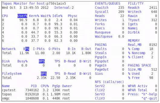
Figure 5-5 Single process - Topas detailed processor statistics
Notice that topas reports CPU0 running at 90.9% in the User% column and only 2.4% in the Idle% column. Also, the Physc values are now spread across CPU0 (0.04), CPU2 (0.01), and CPU3 (0.01), but the sum of the three logical processors still matches the values of the simplified view.
In these examples, it is safe to say that cputest is consuming only 3.2% of the total entitled capacity of the machine.
In an SMT-enabled partition, the SMT distribution over the available cores can also be checked with the mpstat -s command, as shown in Figure 5-6.
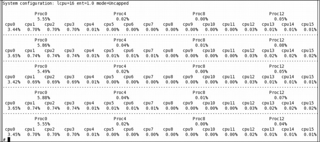
Figure 5-6 mpstat -s reporting a small load on cpu0 and using 5.55% of our entitled capacity
The mpstat -s command gives information about the physical processors (Proc0, Proc4, Proc8, and Proc12) and each of the logical processors (cpu0 through cpu15). Figure 5-6 on page 232 shows five different readings of our system processor while cputest was running.
|
Notes:
•The default behavior of mpstat is to present the results in 80 columns, thus wrapping the lines if you have a lot of processors. The flag -w can be used to display wide lines.
•The additional sections provide some information about SMT systems, focusing on the recent POWER7 SMT4 improvements.
|
5.4.4 Heavy workload example
With the basic processor utilization concepts illustrated, we now take a look at a heavier workload and see how the processor reports changed.
The next examples provide reports of an eight-processes workload with intensive processors.
In Figure 5-7 User% is now reporting almost 90% of processor utilization, but that information itself does not tell much. Physc and Entc% are now reporting much higher values, indicating that the partition is using more of its entitled capacity.
Figure 5-7 Topas simplified processor statistics - Eight simultaneous processes running
Looking at the detailed processor statistics (Figure 5-8), you can see that the physical processor utilization is still spread across the logical processors of the system, and the sum would approximately match the value seen in the simplified view in Figure 5-7.

Figure 5-8 Topas detailed processor statistics - Eight simultaneous processes running
The thread distribution can be seen in Figure 5-9. This partition is an SMT4 partition, and therefore the system tries to distribute the processes as best as possible over the logical processors.

Figure 5-9 mpstat threads view - Eight simultaneous processes running
For the sake of curiosity, Figure 5-10 shows a load of nine processes distributed across only three virtual processors. The interesting detail in this figure is that it illustrates the efforts of the system to make the best use of the SMT4 design by allocating all logical processors of Proc0, Proc4 and Proc2 while Proc6 is almost entirely free.

Figure 5-10 mpstat threads view - Nine simultaneous processes running
5.4.5 Processor utilization reporting in power saving modes
This section shows processor utilization reporting in power saving mode.
Concepts
Before POWER5, AIX calculated processor utilization based on decrementer sampling which is active every tick (10ms). The tick is charged to user/sys/idle/wait buckets, depending on the execution mode when the clock interrupt happens. It is a pure software approach based on the operating system, and not suitable when shared LPAR and SMT are introduced since the physical core is no longer dedicated to one hardware thread.
Since POWER5, IBM introduced Processor Utilization Resource Registers (PURR) for processor utilization accounting. Each processor has one PURR for each hardware thread, and the PURR is counted by hypervisor in fine-grained time slices at nanosecond magnitude. Thus it is more accurate than decrementer sampling, and successfully addresses the utilization reporting issue in SMT and shared LPAR environments.
Since POWER6, IBM introduced power saving features, that is, the processor frequency might vary according to different power saving policies. For example, in static power saving mode, the processor frequency will be at a fixed value lower than nominal; in dynamic power saving mode, the processor frequency can vary dynamically according to the workload, and can reach a value larger than nominal (over-clocking).
Because PURR increments independent of processor frequency, each PURR tick does not necessarily represent the same capacity if you set a specific power saving policy other than the default. To address this problem, POWER6 and later chips introduced the Scaled PURR, which is always proportional to process frequency. When running at lower frequency, the SPURR ticks less than PURR, and when running at higher frequency, the SPURR ticks more than PURR. We can also use SPURR together with PURR to calculate the real operating frequency, as in the equation:
operating frequency = (SPURR/PURR) * nominal frequency
There are several monitoring tools based on SPURR, which can be used to get an accurate utilization of LPARs when in power saving mode. We introduce these tools in the following sections.
Monitor tools
Example 5-25 shows an approach to observe the current power saving policy. You can see that LPAR A is in static power saving mode while LPAR B is in dynamic power saving (favoring performance) mode.
Example 5-25 lparstat -i to observe the power saving policy of an LPAR
LPAR A:
#lparstat -i
…
Power Saving Mode : Static Power Saving
LPAR B:
#lparstat –i
…
Power Saving Mode : Dynamic Power Savings (Favor Performance)
Example 5-26 shows how the processor operating frequency is shown in the lparstat output. There is an extra %nsp column indicating the current ratio compared to nominal processor speed, if the processor is not running at the nominal frequency.
Example 5-26 %nsp in lparstat
#lparstat 1
System configuration: type=Dedicated mode=Capped smt=4 lcpu=32 mem=32768MB
%user %sys %wait %idle %nsp
----- ----- ------ ------ -----
76.7 14.5 5.6 3.1 69
80.0 13.5 4.4 2.1 69
76.7 14.3 5.8 3.2 69
65.2 14.5 13.2 7.1 69
62.6 15.1 14.1 8.1 69
64.0 14.1 13.9 8.0 69
65.0 15.2 12.6 7.2 69
|
Note: If %nsp takes a fixed value lower than 100%, it usually means you have enabled static power saving mode. This might not be what you want, because static power saving mode cannot fully utilize the processor resources despite the workload.
%nsp can also be larger than 100 if the processor is over-clocking in dynamic power saving modes.
|
Example 5-27 shows another lparstat option, -E, for observing the real processor utilization ratio in various power saving modes. As in the output, the actual metrics are based on PURR, while the normalized metrics are based on SPURR. The normalized metrics represent what the real capacity would be if all processors were running at nominal frequency. The sum of user/sys/wait/idle in normalized metrics can exceed the real capacity in case of over-clocking.
Example 5-27 lparstat -E
#lparstat -E 1 100
System configuration: type=Dedicated mode=Capped smt=4 lcpu=64 mem=65536MB Power=Dynamic-Performance
Physical Processor Utilisation:
--------Actual-------- ------Normalised------
user sys wait idle freq user sys wait idle
---- ---- ---- ---- --------- ---- ---- ---- ----
15.99 0.013 0.000 0.000 3.9GHz[102%] 16.24 0.014 0.000 0.000
15.99 0.013 0.000 0.000 3.9GHz[102%] 16.24 0.013 0.000 0.000
15.99 0.009 0.000 0.000 3.9GHz[102%] 16.24 0.009 0.000 0.000 
|
Note: AIX introduces lparstat options -E and -Ew since AIX 5.3 TL9, AIX 6.1 TL2, and AIX 7.1
|
Refer to IBM EnergyScale for POWER7 Processor-Based Systems at:
http://public.dhe.ibm.com/common/ssi/ecm/en/pow03039usen/POW03039USEN.PDF
5.4.6 A common pitfall of shared LPAR processor utilization
For dedicated LPAR, the processor utilization reporting uses the same approach as in no virtualization environment. However, the situation is more complicated in shared LPAR situations. For shared LPAR, if the consumed processor is less than entitlement, the system processor utilization ratio uses the processor entitlement as the base.
As in Example 5-28, %user, %sys, %wait, and %idle are calculated based on the entitled processor, which is 1.00. Thus, 54% user percentage actually means that 0.54 physical processor is consumed in user mode, not 0.54 * 0.86 (physc).
Example 5-28 Processor utilization reporting when consumed processors is less than entitlement
#lparstat 5 3
System configuration: type=Shared mode=Uncapped smt=4 lcpu=16 mem=8192MB psize=16 ent=1.00
%user %sys %wait %idle physc %entc lbusy vcsw phint
----- ----- ------ ------ ----- ----- ------ ----- -----
54.1 0.4 0.0 45.5 0.86 86.0 7.3 338 0
54.0 0.3 0.0 45.7 0.86 85.7 6.8 311 0
54.0 0.3 0.0 45.7 0.86 85.6 7.2 295 0
If the consumed processor is larger than entitlement, the system processor utilization ratio uses the consumed processor as the base. Refer to Example 5-29 on page 237. In this case, %usr, %sys, %wait, and %idle are calculated based on the consumed processor. Thus 62.2% user percentage actually means that 2.01*0.622 processor is consumed in user mode.
Example 5-29 Processor utilization reporting when consumed processors exceeds entitlement
#lparstat 5 3
System configuration: type=Shared mode=Uncapped smt=4 lcpu=16 mem=8192MB psize=16 ent=1.00
%user %sys %wait %idle physc %entc lbusy vcsw phint
----- ----- ------ ------ ----- ----- ------ ----- -----
62.3 0.2 0.0 37.6 2.00 200.3 13.5 430 0
62.2 0.2 0.0 37.6 2.01 200.8 12.7 569 0
62.2 0.2 0.0 37.7 2.01 200.7 13.4 550 0
|
Note: The rule above applies to overall system processor utilization reporting. The specific logical processor utilization ratios in sar -P ALL and mpstat -a are always based on their physical consumed processors. However, the overall processor utilization reporting in these tools still complies with the rule.
|
5.5 Memory utilization
This section covers a suggested approach of looking at memory usage, how to read the metrics correctly and how to understand paging space utilization. It shows how to monitor memory in partitions with dedicated memory, active memory sharing, and active memory expansion. It also presents some information about memory leaks and memory size simulation.
5.5.1 How much memory is free (dedicated memory partitions)
In AIX, memory requests are managed by the Virtual Memory Manager (VMM). Virtual memory includes real physical memory (RAM) and memory stored on disk (paging space).
Virtual memory segments are partitioned into fixed-size units called pages. AIX supports four page sizes: 4 KB, 64 KB, 16 MB and 16 GB. The default page size is 4 KB. When free memory becomes low, VMM uses the Last Recently Used (LRU) algorithm to replace less frequently referenced memory pages to paging space. To optimize which pages are candidates for replacement, AIX classifies them into two types:
•Computational memory
•Non-computational memory
Computational memory, also known as computational pages, consists of the pages that belong to working-storage segments or program text (executable files) segments. Non-computational memory or file memory is usually pages from permanent data files in persistent storage.
AIX tends to use all of the physical memory available. Depending on how you look at your memory utilization, you may think you need more memory.
In Example 5-30, the fre column shows 8049 pages of 4 KB of free memory = 31 MB and the LPAR has 8192 MB. Apparently, the system has almost no free memory.
Example 5-30 vmstat shows there is almost no free memory
# vmstat
System configuration: lcpu=16 mem=8192MB ent=1.00
kthr memory page faults cpu
----- ----------- ------------------------ ------------ -----------------------
r b avm fre re pi po fr sr cy in sy cs us sy id wa pc ec
1 1 399550 8049 0 0 0 434 468 0 68 3487 412 0 0 99 0 0.00 0.0
Using the command dd if=/dev/zero of=/tmp/bigfile bs=1M count=8192, we generated a file of the size of our RAM memory (8192 MB). The output of vmstat in Example 5-31 presents 6867 frames of 4 k free memory = 26 MB.
Example 5-31 vmstat still shows almost no free memory
kthr memory page faults cpu
----- ----------- ------------------------ ------------ -----------------------
r b avm fre re pi po fr sr cy in sy cs us sy id wa pc ec
1 1 399538 6867 0 0 0 475 503 0 60 2484 386 0 0 99 0 0.000 0.0
Looking at the memory report of topas, Example 5-32, you see that the non-computational memory, represented by Noncomp, is 80%.
Example 5-32 Topas shows non-computational memory at 80%
Topas Monitor for host:p750s2aix4 EVENTS/QUEUES FILE/TTY
Thu Oct 11 18:46:27 2012 Interval:2 Cswitch 271 Readch 3288
Syscall 229 Writech 380
CPU User% Kern% Wait% Idle% Physc Entc% Reads 38 Rawin 0
Total 0.1 0.3 0.0 99.6 0.01 0.88 Writes 0 Ttyout 178
Forks 0 Igets 0
Network BPS I-Pkts O-Pkts B-In B-Out Execs 0 Namei 23
Total 1.01K 9.00 2.00 705.0 330.0 Runqueue 0.50 Dirblk 0
Waitqueue 0.0
Disk Busy% BPS TPS B-Read B-Writ MEMORY
Total 0.0 0 0 0 0 PAGING Real,MB 8192
Faults 0 % Comp 19
FileSystem BPS TPS B-Read B-Writ Steals 0 % Noncomp 80
Total 3.21K 38.50 3.21K 0 PgspIn 0 % Client 80
PgspOut 0
Name PID CPU% PgSp Owner PageIn 0 PAGING SPACE
topas 5701752 0.1 2.48M root PageOut 0 Size,MB 2560
java 4456586 0.1 20.7M root Sios 0 % Used 0
getty 5308512 0.0 640K root % Free 100
gil 2162754 0.0 960K root NFS (calls/sec)
slp_srvr 4915352 0.0 472K root SerV2 0 WPAR Activ 0
java 7536870 0.0 55.7M pconsole CliV2 0 WPAR Total 1
pcmsrv 8323232 0.0 1.16M root SerV3 0 Press: "h"-help
java 6095020 0.0 64.8M root CliV3 0 "q"-quit
After using the command rm /tmp/bigfile, we saw that the vmstat output, shown in Example 5-33, shows 1690510 frames of 4 k free memory = 6603 MB.
Example 5-33 vmstat shows a lot of free memory
kthr memory page faults cpu
----- ----------- ------------------------ ------------ -----------------------
r b avm fre re pi po fr sr cy in sy cs us sy id wa pc ec
1 1 401118 1690510 0 0 0 263 279 0 35 1606 329 0 0 99 0 0.000 0.0
What happened with the memory after we issued the rm command? Remember non-computational memory? It is basically file system cache. Our dd filled the non-computational memory and rm wipes that cache from noncomp memory.
AIX VMM keeps a free list—real memory pages that are available to be allocated. When process requests memory and there are not sufficient pages in the free list, AIX first removes pages from non-computational memory.
Many monitoring tools present the utilized memory without discounting non-computational memory. This leads to potential misunderstanding of statistics and incorrect assumptions about how much of memory is actually free. In most cases it should be possible to make adjustments to give the right value.
In order to know the utilized memory, the correct column to look at, when using vmstat, is active virtual memory (avm). This value is also presented in 4 KB pages. In Example 5-30 on page 237, while the fre column of vmstat shows 8049 frames (31 MB), the avm is 399,550 pages (1560 MB). For 1560 MB used out of 8192 MB of the total memory of the LPAR, there are 6632 MB free. The avm value can be greater than the physical memory, because some pages might be in RAM and others in paging space. If that happens, it is an indication that your workload requires more than the physical memory available.
Let us play more with dd and this time analyze memory with topas. In Example 5-34, topas output shows 1% utilization of Noncomp (non-computational) memory.
Using the dd command again:
dd if=/dev/zero of=/tmp/bigfile bs=1M count=8192
The topas output in Example 5-34 shows that the sum of computational and non-computational memory is 99%, so almost no memory is free. What will happen if you start a program that requests memory? To illustrate this, in Example 5-35, we used the stress tool from:
Example 5-34 Topas shows Comp + Noncomp = 99% (parts stripped for better reading)
Disk Busy% BPS TPS B-Read B-Writ MEMORY
Total 0.0 0 0 0 0 PAGING Real,MB 8192
Faults 78 % Comp 23
FileSystem BPS TPS B-Read B-Writ Steals 0 % Noncomp 76
Total 2.43K 28.50 2.43K 0 PgspIn 0 % Client 76
Example 5-35 Starting a program that requires 1024 MB of memory
# stress --vm 1 --vm-bytes 1024M --vm-hang 0
stress: info: [11600010] dispatching hogs: 0 cpu, 0 io, 1 vm, 0 hdd
In Example 5-36, non-computational memory dropped from 76% (Example 5-34) to 63% and the computational memory increased from 23% to 35%.
Example 5-36 Topas output while running a stress program
Disk Busy% BPS TPS B-Read B-Writ MEMORY
Total 0.0 0 0 0 0 PAGING Real,MB 8192
Faults 473 % Comp 35
FileSystem BPS TPS B-Read B-Writ Steals 0 % Noncomp 63
After cancelling the stress program, Example 5-37 shows that non-computational memory remains at the same value and the computational returned to the previous mark. This shows that when a program requests computational memory, VMM allocates this memory as computational and releases pages from non-computational.
Example 5-37 Topas after cancelling the program
Disk Busy% BPS TPS B-Read B-Writ MEMORY
Total 0.0 0 0 0 0 PAGING Real,MB 8192
Faults 476 % Comp 23
FileSystem BPS TPS B-Read B-Writ Steals 0 % Noncomp 63
Using nmon, in Example 5-38, the sum of the values Process and System is approximately the value of Comp. Process is memory utilized by the application process and System is memory utilized by the AIX kernel.
Example 5-38 Using nmon to analyze memory
??topas_nmon??b=Black&White??????Host=p750s2aix4?????Refresh=2 secs???18:49.27??
? Memory ???????????????????????????????????????????????????????????????????????
? Physical PageSpace | pages/sec In Out | FileSystemCache?
?% Used 89.4% 2.4% | to Paging Space 0.0 0.0 | (numperm) 64.5%?
?% Free 10.6% 97.6% | to File System 0.0 0.0 | Process 15.7%?
?MB Used 7325.5MB 12.1MB | Page Scans 0.0 | System 9.2%?
?MB Free 866.5MB 499.9MB | Page Cycles 0.0 | Free 10.6%?
?Total(MB) 8192.0MB 512.0MB | Page Steals 0.0 | -----?
? | Page Faults 0.0 | Total 100.0%?
?------------------------------------------------------------ | numclient 64.5%?
?Min/Maxperm 229MB( 3%) 6858MB( 90%) <--% of RAM | maxclient 90.0%?
?Min/Maxfree 960 1088 Total Virtual 8.5GB | User 73.7%?
?Min/Maxpgahead 2 8 Accessed Virtual 2.0GB 23.2%| Pinned 16.2%?
? | lruable pages ?
????????????????????????????????????????????????????????????????????????????????
svmon
Another useful tool to see how much memory is free is svmon. Since AIX 5.3 TL9 and AIX 6.1 TL2, svmon has a new metric called available memory, representing the free memory. Example 5-39 shows svmon output. The available memory is 5.77 GB.
Example 5-39 svmon output shows available memory
# svmon -O summary=basic,unit=auto
Unit: auto
--------------------------------------------------------------------------------------
size inuse free pin virtual available mmode
memory 8.00G 7.15G 873.36M 1.29G 1.97G 5.77G Ded
pg space 512.00M 12.0M
work pers clnt other
pin 796.61M 0K 0K 529.31M
in use 1.96G 0K 5.18G
One svmon usage is to show the top 10 processes in memory utilization, shown in Example 5-40 on page 241.
Example 5-40 svmon - top 10 memory consuming processes
# svmon -Pt10 -O unit=KB
Unit: KB
-------------------------------------------------------------------------------
Pid Command Inuse Pin Pgsp Virtual
5898490 java 222856 40080 0 194168
7536820 java 214432 40180 0 179176
6947038 cimserver 130012 39964 0 129940
8126526 cimprovagt 112808 39836 0 112704
8519700 cimlistener 109496 39836 0 109424
6488292 rmcd 107540 39852 0 106876
4063360 tier1slp 106912 39824 0 106876
5636278 rpc.statd 102948 39836 0 102872
6815958 topasrec 102696 39824 0 100856
6357198 IBM.DRMd 102152 39912 0 102004
Example 5-41 svmon showing only Java processes
# svmon -C java -O unit=KB,process=on
Unit: KB
===============================================================================
Command Inuse Pin Pgsp Virtual
java 236568 39376 106200 312868
-------------------------------------------------------------------------------
Pid Command Inuse Pin Pgsp Virtual
7274720 java 191728 38864 9124 200836
6553820 java 38712 372 74956 88852
4915426 java 6128 140 22120 23180
For additional information, refer to:
aix4admins.blogspot.com/2011/09/vmm-concepts-virtual-memory-segments.html
or
www.ibm.com/developerworks/aix/library/au-vmm/
Example 5-42 Output of the vmstat - v command
# vmstat -v
2097152 memory pages
1950736 lruable pages
223445 free pages
2 memory pools
339861 pinned pages
90.0 maxpin percentage
3.0 minperm percentage
90.0 maxperm percentage
69.3 numperm percentage
1352456 file pages
0.0 compressed percentage
0 compressed pages
69.3 numclient percentage
90.0 maxclient percentage
1352456 client pages
0 remote pageouts scheduled
0 pending disk I/Os blocked with no pbuf
191413 paging space I/Os blocked with no psbuf
2228 filesystem I/Os blocked with no fsbuf
0 client filesystem I/Os blocked with no fsbuf
2208 external pager filesystem I/Os blocked with no fsbuf
24.9 percentage of memory used for computational pages
The vmstat command in Example 5-42 on page 241 shows: 1352456 client pages - non-computational, 1359411 - 1352456 = 6955.
Example 5-43 Output of the svmon command
# svmon -O summary=basic
Unit: page
--------------------------------------------------------------------------------------
size inuse free pin virtual available mmode
memory 2097152 1873794 223358 339861 515260 1513453 Ded
pg space 131072 3067
work pers clnt other
pin 204357 0 0 135504
in use 514383 0 1359411
The output of the svmon command in Example 5-43 shows: 1359411 client pages. Some of them are computational and the rest are non-computational.
5.5.2 Active memory sharing partition monitoring
This section shows how to monitor the memory in shared memory partitions. It can be done with the vmstat, lparstat, topas commands, and so on, and these commands with the -h option show hypervisor paging information.
The operating system sees a logical entity that is not always backed up with physical memory.
When using the vmstat command with the -h option, the hypervisor paging information will be displayed as shown in Example 5-44.
Example 5-44 vmstat with hypervisor
# vmstat -h 5 3
System configuration: lcpu=16 mem=8192MB ent=1.00 mmode=shared mpsz=8.00GB
kthr memory page faults cpu hypv-page
----- ----------- ------------------------ ------------ ----------------------- -------------------------
r b avm fre re pi po fr sr cy in sy cs us sy id wa pc ec hpi hpit pmem loan
0 0 399386 1666515 0 0 0 0 0 0 3 124 120 0 0 99 0 0.00 0.4 0 0 8.00 0.00
In this case, It also shows the number of 4 KB pages in avm, fri and page columns
It shows 6G or more of free space (ie. 1666515 * 4k pages)
mmode Shows shared if the partition is running in shared memory mode. This field was not displayed on dedicated memory partitions.
mpsz Shows the size of the shared memory pool.
hpi Shows the number of hypervisor page-ins for the partition. A hypervisor page-in occurs if a page is being referenced that is not available in real memory because it has been paged out by the hypervisor previously. If no interval is specified when issuing the vmstat command, the value shown is counted from boot time.
hpit Shows the average time spent in milliseconds per hypervisor page-in. If no interval is specified when issuing the vmstat command, the value shown is counted from boot time.
pmem Shows the amount of physical memory backing the logical memory, in gigabytes.
loan Shows the amount of the logical memory in gigabytes that is loaned to the hypervisor. The amount of loaned memory can be influenced through the vmo ams_loan_policy tunable.
If the consumed memory is larger than the desired memory, the system utilization avm ratio is over desired memory capacity, as shown in Example 5-45.
Example 5-45 In case of larger than desired memory consumption (vmstat with hypervisor)
# vmstat -h 5 3
System configuration: lcpu=16 mem=8192MB ent=1.00 mmode=shared mpsz=8.00GB
kthr memory page faults cpu hypv-page
----- ----------- ------------------------ ------------ ----------------------------- -------------------------
r b avm fre re pi po fr sr cy in sy cs us sy id wa pc ec hpi hpit pmem loan
7 3 1657065 3840 0 0 0 115709 115712 0 3 16 622057 45 24 15 17 3.75 374.9 0 0 8.00 0.00
7 3 2192911 4226 0 7 16747 102883 153553 0 1665 10 482975 41 26 18 15 3.19 318.6 0 0 8.00 0.00
5 6 2501329 5954 0 48 54002 53855 99595 0 6166 11 36778 25 43 25 6 1.12 112.2 0 0 8.00 0.00
If loaning is enabled (ams_loan_policy is set to 1 or 2 in vmo), AIX loans pages when the hypervisor initiates a request. AIX removes free pages that are loaned to the hypervisor from the free list.
Example 5-44 on page 242 shows a partition that has a logical memory size of 8 GB. It has also assigned 8 GB of physical memory. Of this assigned 8 GB of physical memory, 6.3 GB (1666515 4 k pages) are free because there is no activity in the partition.
Example 5-46 shows the same partition a few minutes later. In the meantime, the hypervisor requested memory and the partition loaned 3.2 GB to the hypervisor. AIX has removed the free pages that it loaned from the free list.
Example 5-46 vmstat command
# vmstat -h 5 3
System configuration: lcpu=16 mem=8192MB ent=1.00 mmode=shared mpsz=8.00GB
kthr memory page faults cpu hypv-page
----- ----------- ------------------------ ------------ ----------------------- -------------------------
r b avm fre re pi po fr sr cy in sy cs us sy id wa pc ec hpi hpit pmem loan
0 0 399386 833215 0 0 0 0 0 0 3 124 120 0 0 99 0 0.00 0.4 0 0 4.76 3.24
AIX paging and hypervisor paging
When using active memory sharing, paging can occur on the AIX level or on the hypervisor level. When you see non-zero values in the pi or po column of the vmstat command, it means that AIX is performing paging activities.
In a shared memory partition, AIX paging occurs not only when the working set exceeds the size of the logical memory, as in a dedicated partition. This can happen even if the LPAR has less physical memory than logical memory. AIX is dependent on the amount of logical memory available.
Another reason is that AIX is freeing memory pages to loan them to the hypervisor. If the loaned pages are used pages, AIX has to save the content to its paging space before loaning them to the hypervisor.
This behavior will especially occur if you have selected an aggressive loaning policy (ams_loan_policy=2).
5.5.3 Active memory expansion partition monitoring
In 3.2, “Active Memory Expansion” on page 48, the concepts of active memory expansion (AME) were introduced. Now, a few examples of how to monitor AME behavior are shown.
Monitoring of AME can be done with the special tools amepat, topas -L.
The amepat command
The amepat command provides a summary of the active memory expansion configuration, and can be used for monitoring and fine-tuning the configuration.
The amepat command shows the current configuration and statistics of the system resource utilization over the monitoring period. It can be run for periods of time to collect metrics while a workload is running, as shown in Example 5-47.
Example 5-47 amepat with little memory consumption
# amepat 1 5
Command Invoked : amepat 1 5
Date/Time of invocation : Wed Oct 10 10:33:13 CDT 2012
Total Monitored time : 5 mins 6 secs
Total Samples Collected : 5
System Configuration:
---------------------
Partition Name : p750s1aix4
Processor Implementation Mode : POWER7 Mode
Number Of Logical CPUs : 16
Processor Entitled Capacity : 1.00
Processor Max. Capacity : 4.00
True Memory : 8.00 GB
SMT Threads : 4
Shared Processor Mode : Enabled-Uncapped
Active Memory Sharing : Disabled
Active Memory Expansion : Disabled
System Resource Statistics: Average Min Max
--------------------------- ----------- ----------- -----------
CPU Util (Phys. Processors) 0.00 [ 0%] 0.00 [ 0%] 0.00 [ 0%]
Virtual Memory Size (MB) 1564 [ 19%] 1564 [ 19%] 1564 [ 19%]
True Memory In-Use (MB) 1513 [ 18%] 1513 [ 18%] 1514 [ 18%]
Pinned Memory (MB) 1443 [ 18%] 1443 [ 18%] 1443 [ 18%]
File Cache Size (MB) 19 [ 0%] 19 [ 0%] 19 [ 0%]
Available Memory (MB) 6662 [ 81%] 6662 [ 81%] 6663 [ 81%]
Active Memory Expansion Modeled Statistics :
-------------------------------------------
Modeled Expanded Memory Size : 8.00 GB
Achievable Compression ratio :1.90
Expansion Modeled True Modeled CPU Usage
Factor Memory Size Memory Gain Estimate
--------- ------------- ------------------ -----------
1.00 8.00 GB 0.00 KB [ 0%] 0.00 [ 0%]
1.11 7.25 GB 768.00 MB [ 10%] 0.00 [ 0%]
1.19 6.75 GB 1.25 GB [ 19%] 0.00 [ 0%]
1.28 6.25 GB 1.75 GB [ 28%] 0.00 [ 0%]
1.34 6.00 GB 2.00 GB [ 33%] 0.00 [ 0%]
1.46 5.50 GB 2.50 GB [ 45%] 0.00 [ 0%]
1.53 5.25 GB 2.75 GB [ 52%] 0.00 [ 0%]
Active Memory Expansion Recommendation:
---------------------------------------
The recommended AME configuration for this workload is to configure the LPAR
with a memory size of 5.25 GB and to configure a memory expansion factor
of 1.53. This will result in a memory gain of 52%. With this
configuration, the estimated CPU usage due to AME is approximately 0.00
physical processors, and the estimated overall peak CPU resource required for
the LPAR is 0.00 physical processors.
NOTE: amepat's recommendations are based on the workload's utilization level
during the monitored period. If there is a change in the workload's utilization
level or a change in workload itself, amepat should be run again.
The modeled Active Memory Expansion CPU usage reported by amepat is just an
estimate. The actual CPU usage used for Active Memory Expansion may be lower
or higher depending on the workload.
Example 5-48 shows amepat with heavy memory consumption. It shows a high memory compression ratio because the test program consumes garbage memory.
Example 5-48 The amepat command
# amepat 1 5
Command Invoked : amepat 1 5
Date/Time of invocation : Wed Oct 10 11:36:07 CDT 2012
Total Monitored time : 6 mins 2 secs
Total Samples Collected : 5
System Configuration:
---------------------
Partition Name : p750s1aix4
Processor Implementation Mode : POWER7 Mode
Number Of Logical CPUs : 16
Processor Entitled Capacity : 1.00
Processor Max. Capacity : 4.00
True Memory : 8.00 GB
SMT Threads : 4
Shared Processor Mode : Enabled-Uncapped
Active Memory Sharing : Disabled
Active Memory Expansion : Disabled
System Resource Statistics: Average Min Max
--------------------------- ----------- ----------- -----------
CPU Util (Phys. Processors) 0.13 [ 3%] 0.00 [ 0%] 0.31 [ 8%]
Virtual Memory Size (MB) 6317 [ 77%] 2592 [ 32%] 9773 [119%]
True Memory In-Use (MB) 5922 [ 72%] 2546 [ 31%] 8178 [100%]
Pinned Memory (MB) 1454 [ 18%] 1447 [ 18%] 1460 [ 18%]
File Cache Size (MB) 296 [ 4%] 23 [ 0%] 1389 [ 17%]
Available Memory (MB) 2487 [ 30%] 6 [ 0%] 5630 [ 69%]
Active Memory Expansion Modeled Statistics :
-------------------------------------------
Modeled Expanded Memory Size : 8.00 GB
Achievable Compression ratio :6.63
Expansion Modeled True Modeled CPU Usage
Factor Memory Size Memory Gain Estimate
--------- ------------- ------------------ -----------
1.04 7.75 GB 256.00 MB [ 3%] 0.00 [ 0%]
1.34 6.00 GB 2.00 GB [ 33%] 0.00 [ 0%]
1.69 4.75 GB 3.25 GB [ 68%] 0.00 [ 0%]
2.00 4.00 GB 4.00 GB [100%] 0.00 [ 0%]
2.29 3.50 GB 4.50 GB [129%] 0.00 [ 0%]
2.67 3.00 GB 5.00 GB [167%] 0.00 [ 0%]
2.91 2.75 GB 5.25 GB [191%] 0.00 [ 0%]
Active Memory Expansion Recommendation:
---------------------------------------
The recommended AME configuration for this workload is to configure the LPAR
with a memory size of 2.75 GB and to configure a memory expansion factor
of 2.91. This will result in a memory gain of 191%. With this
configuration, the estimated CPU usage due to AME is approximately 0.00
physical processors, and the estimated overall peak CPU resource required for
the LPAR is 0.31 physical processors.
NOTE: amepat's recommendations are based on the workload's utilization level
during the monitored period. If there is a change in the workload's utilization
level or a change in workload itself, amepat should be run again.
The modeled Active Memory Expansion CPU usage reported by amepat is just an
estimate. The actual CPU usage used for Active Memory Expansion may be lower
or higher depending on the workload.
The topas command
The topas command shows the following active memory expansion metrics on the default panel when started with no options:
•TMEM, MB - True memory size in megabytes.
•CMEM, MB - Compressed pool size in megabytes.
•EF[T/A] - Expansion factors: Target and Actual.
•CI - Compressed pool page-ins.
•CO - Compressed pool page-outs.
Example 5-49 Monitoring active memory expansion with the topas command
Topas Monitor for host:p750s1aix4 EVENTS/QUEUES FILE/TTY
Wed Oct 10 13:31:19 2012 Interval:FROZEN Cswitch 4806.0M Readch 3353.8G
Syscall 1578.4M Writech 3248.8G
CPU User% Kern% Wait% Idle% Physc Entc% Reads 49.8M Rawin 642.2K
Total 38.1 61.9 0.0 0.0 2.62 262.41 Writes 101.6M Ttyout 25.5M
Forks 1404.8K Igets 4730
Network BPS I-Pkts O-Pkts B-In B-Out Execs 1463.8K Namei 110.2M
Total 0 0 0 0 0 Runqueue 3.00M Dirblk 95749
Waitqueue 65384.6
Disk Busy% BPS TPS B-Read B-Writ MEMORY
Total 0.0 0 0 0 0 PAGING Real,MB 8192
Faults 2052.0M % Comp 18
FileSystem BPS TPS B-Read B-Writ Steals 802.8M % Noncomp 0
Total 2.52M 2.52K 2.52M 0 PgspIn 547.4K % Client 0
PgspOut 126.3M
Name PID CPU% PgSp Owner PageIn 4204.6K PAGING SPACE
inetd 4718746 0.0 536K root PageOut 936.4M Size,MB 8192
lrud 262152 0.0 640K root Sios 908.0M % Used 1
hostmibd 4784176 0.0 1.12M root % Free 99
psmd 393228 0.0 640K root AME
aixmibd 4849826 0.0 1.30M root TMEM,MB 2815.2M WPAR Activ 0
hrd 4915356 0.0 924K root CMEM,MB 1315.7M WPAR Total 0
reaffin 589842 0.0 640K root EF[T/A] 2.91 Press: "h"-help
sendmail 4980888 0.0 1.05M root CI:0.0KCO:0.1K "q"-quit
lvmbb 720920 0.0 448K root
vtiol 786456 0.0 1.06M root
ksh 6226074 0.0 556K root
pilegc 917532 0.0 640K root
xmgc 983070 0.0 448K root
5.5.4 Paging space utilization
When a program requests some memory and that amount cannot be satisfied in RAM, the Virtual Memory Manager (VMM), through the last recently used (lru) algorithm, selects some pages to be moved to paging space, also called swap space. This is called a page-out. This allows the memory request to be fulfilled. When these pages in swap are needed again, they are read from hard disk and moved back into RAM. This is called page-in.
Excess of paging is bad for performance because access to paging devices (disks) is many times slower than access to RAM. Therefore, it is important to have a good paging setup, as shown in 4.2.2, “Paging space” on page 128, and to monitor the paging activity.
Beginners in AIX think that if they look at the paging space utilization and see a high number, that is bad. Looking at the output of lsps -a and having a paging space utilization greater than zero, does not mean that AIX is memory constraint at the moment.
|
Tip: It is safer to use the lsps -s command rather than the lsps -a.
|
Example 5-50 shows paging space utilization at 71%. However, this does not mean that AIX is paging or that the system has low free memory available. In Example 5-51, the output of svmon shows 6168.44 MB of available memory and 1810.98 MB of paging space used.
Example 5-50 Looking at paging space utilization
# lsps -a
Page Space Physical Volume Volume Group Size %Used Active Auto Type Chksum
hd6 hdisk0 rootvg 2560MB 71 yes yes lv 0
Example 5-51 Available memory and paging utilization
# svmon -O summary=basic,unit=MB
Unit: MB
--------------------------------------------------------------------------------------
size inuse free pin virtual available mmode
memory 8192.00 2008.56 6183.44 1208.25 3627.14 6168.44 Ded
pg space 2560.00 1810.98
work pers clnt other
pin 678.94 0 0 529.31
in use 1835.16 0 173.40
The percent paging space utilization means that at some moment AIX VMM required that amount of paging. After this peak of memory requirements, some process that had pages paged out did not require a page-in of such pages, or if the page-in was required, it was for read access and not for modifying. Paging space garbage collection, by default, only operates when a page-in happens. If the page is brought back into memory to read-only operations, it is not freed up from paging space. This provides better performance because if the page remains unmodified and is stolen from RAM by the LRU daemon, it is not necessary to perform the repage-out function.
One important metric regarding paging is paging in and paging out. In Example 5-52 using topas we see AIX during a low paging activity. PgspIn is the number of 4 K pages read from paging space per second over the monitoring interval. PgspOut is the number of 4 K pages written to paging space per second over the monitoring interval.
Example 5-52 topas showing small paging activity
Topas Monitor for host:p750s2aix4 EVENTS/QUEUES FILE/TTY
Mon Oct 8 18:52:33 2012 Interval:2 Cswitch 400 Readch 2541
Syscall 227 Writech 512
CPU User% Kern% Wait% Idle% Physc Entc% Reads 28 Rawin 0
Total 0.2 0.5 0.0 99.3 0.01 1.36 Writes 1 Ttyout 246
Forks 0 Igets 0
Network BPS I-Pkts O-Pkts B-In B-Out Execs 0 Namei 24
Total 677.0 4.00 2.00 246.0 431.0 Runqueue 1.00 Dirblk 0
Waitqueue 0.0
Disk Busy% BPS TPS B-Read B-Writ MEMORY
Total 0.0 458K 81.50 298K 160K PAGING Real,MB 8192
Faults 88 % Comp 98
FileSystem BPS TPS B-Read B-Writ Steals 40 % Noncomp 1
Total 2.48K 28.50 2.48K 0 PgspIn 74 % Client 1
PgspOut 40
Name PID CPU% PgSp Owner PageIn 74 PAGING SPACE
java 8388796 0.5 65.2M root PageOut 40 Size,MB 2560
syncd 786530 0.2 596K root Sios 87 % Used 89
java 6553710 0.1 21.0M root % Free 11
topas 7995432 0.1 2.04M root NFS (calls/sec)
lrud 262152 0.0 640K root SerV2 0 WPAR Activ 0
getty 6815754 0.0 640K root CliV2 0 WPAR Total 1
vtiol 851994 0.0 1.06M root SerV3 0 Press: "h"-help
gil 2162754 0.0 960K root CliV3 0 "q"-quit
Example 5-53 vmstat showing considerable paging activity
# vmstat 5
System configuration: lcpu=16 mem=8192MB ent=1.00
kthr memory page faults cpu
----- ----------- ------------------------ ------------ -----------------------
r b avm fre re pi po fr sr cy in sy cs us sy id wa pc ec
2 0 2241947 5555 0 3468 3448 3448 3448 0 3673 216 7489 9 4 84 3 0.26 26.0
2 0 2241948 5501 0 5230 5219 5219 5222 0 5521 373 11150 14 6 71 9 0.39 38.6
2 1 2241948 5444 0 5156 5145 5145 5145 0 5439 83 10972 14 6 76 4 0.40 40.1
1 0 2241959 5441 0 5270 5272 5272 5272 0 5564 435 11206 14 6 70 9 0.39 38.9
1 1 2241959 5589 0 5248 5278 5278 5278 0 5546 82 11218 14 6 76 4 0.41 40.9
If your system is consistently presenting high page-in or page-out rates, your performance is probably being affected due to memory constraints.
5.5.5 Memory size simulation with rmss
It is possible to simulate reduced sizes of memory without performing a dlpar operation and without stopping the partition. The rmss command—reduced memory system simulator—can be used to test application and system behavior with different memory scenarios.
The main use for the rmss command is as a capacity planning tool to determine how much memory a workload needs.
To determine whether the rmss command is installed and available, run the following command:
# lslpp -lI bos.perf.tools
You can use the rmss command in two modes:
•To change the system memory size.
•To execute a specified application multiple times over a range of memory sizes and display important statistics that describe the application's performance at each memory size.
Example 5-54 Using rmss to simulate a system with 4 GB memory
# rmss -c 4096
Simulated memory size changed to 4096 Mb.
Warning: This operation might impact the system environment.
Please refer vmo documentation to resize the appropriate parameters.
The simulated memory can be verified with the -p flag; to reset to physical real memory, use the -r flag.
5.5.6 Memory leaks
Memory leak is a software error in which the program allocates memory and never releases it after use. In a long-running program, memory leak is a serious problem because it can exhaust the system real memory and paging space, leading to a program or system crash.
Memory leaks are not to be confused with caching or any other application behavior. Processes showing an increase in memory consumption may not be leaking memory. Instead, that can actually be the expected behavior, depending on what the program is intended to do.
Before continuing, it must be clear that memory leaks can only be confirmed with source code analysis. However, some system analysis may help in identifying possible programs with problems.
A memory leak can be detected with the ps command, using the v flag. This flag displays a SIZE column, which shows the virtual size of the data section of the process.
|
Note: The SIZE column does not represent the same as the SZ column produced by the -l flag. Although sometimes they show the same value, they can be different if some pages of the process are paged out.
|
Using ps, the information of a process with pid 6291686 is collected at 30-second intervals, as seen in Example 5-55.
Example 5-55 Using ps to collect memory information
# while true ; do ps v 6291686 >> /tmp/ps.out ; sleep 30 ; done
Example 5-56 Increase in memory utilization
# grep PID /tmp/ps.out | head -n 1 ; grep 6291686 /tmp/ps.out
PID TTY STAT TIME PGIN SIZE RSS LIM TSIZ TRS %CPU %MEM COMMAND
6291686 pts/2 A 0:00 0 156 164 xx 1 8 0.0 0.0 ./test_
6291686 pts/2 A 0:00 0 156 164 xx 1 8 0.0 0.0 ./test_
6291686 pts/2 A 0:00 0 160 168 xx 1 8 0.0 0.0 ./test_
6291686 pts/2 A 0:00 0 164 172 xx 1 8 0.0 0.0 ./test_
6291686 pts/2 A 0:00 0 164 172 xx 1 8 0.0 0.0 ./test_
6291686 pts/2 A 0:00 0 168 176 xx 1 8 0.0 0.0 ./test_
6291686 pts/2 A 0:00 0 172 180 xx 1 8 0.0 0.0 ./test_
Another command that can be used is svmon, which looks for processes whose working segment continually grows. To determine whether a segment is growing, use svmon with the -i <interval> option to look at a process or a group of processes and see whether any segment continues to grow.
Example 5-57 shows how to start collecting data with svmon. Example 5-58 shows the increase in size for segment 2 (Esid 2 - process private).
Example 5-57 Using svmon to collect memory information
# svmon -P 6291686 -i 30 > /tmp/svmon.out
Example 5-58 Output of svmon showing increase in memory utilization
# grep Esid /tmp/svmon.out | head -n 1 ; grep " 2 work" /tmp/svmon.out
Vsid Esid Type Description PSize Inuse Pin Pgsp Virtual
9a0dba 2 work process private sm 20 4 0 20
9a0dba 2 work process private sm 20 4 0 20
9a0dba 2 work process private sm 21 4 0 21
9a0dba 2 work process private sm 22 4 0 22
9a0dba 2 work process private sm 22 4 0 22
9a0dba 2 work process private sm 23 4 0 23
9a0dba 2 work process private sm 24 4 0 24
9a0dba 2 work process private sm 24 4 0 24
|
Important: Never assume that a program is leaking memory only by monitoring the operating system. Source code analysis must always be conducted to confirm the problem.
|
5.6 Disk storage bottleneck identification
When finding that there is a performance bottleneck related to external disk storage, it can be challenging to find the source of the problem. It can be in any component of the server, SAN or storage infrastructures. This section explains some of the performance metrics to look at when diagnosing a performance problem, and where to look in the event that you have an I/O performance problem.
5.6.1 Performance metrics
There are different metrics to consider when looking at the disk utilization of an AIX system. To identify a bottleneck, you first need to understand the metrics involved to be able to identify a problem.
Table 5-3 gives a summary of key performance metrics to understand when investigating an I/O performance problem on an AIX system.
Table 5-3 Key performance metrics
|
Metric
|
Description
|
|
IOPS
|
IOPS represents the amount of read or write I/O operations performed in a 1-second time interval.
|
|
Throughput
|
Throughput is the amount of data that can be transferred between the server and the storage measured in megabytes per second.
|
|
Transfer size
|
The transfer size typically measured in kilobytes is the size of an I/O request.
|
|
Wait time
|
Wait time is the amount of time measured in milliseconds that the server’s processor has to wait for a pending I/O to complete. The pending I/O could be in the queue for the I/O device, increasing the wait time for an I/O request.
|
|
Service time
|
Service time is the time taken for the storage system to service an I/O transfer request in milliseconds.
|
Depending on the type of I/O that is being performed, the service times may differ. An I/O operation with a small transfer size would be expected to have a significantly smaller service time than an I/O with a large transfer size because the larger I/O operation is bigger and more data has to be processed to service it. Larger I/O operations are also typically limited to throughput. For instance, the service time of a 32 k I/O will be significantly larger than an 8 k I/O because the 32 k I/O is four times the size of the 8 k I/O.
When trying to identify a performance bottleneck it is necessary to understand whether the part of your workload that may not be performing adequately (for example, a batch job) is using small block random I/O or large block sequential I/O.
5.6.2 Additional workload and performance implications
A storage system, dependant on its configuration, will be able to sustain a certain amount of workload until at some point one or more components become saturated and the service time, also known as response time, increases exponentially.
It is important to understand the capability of the storage system that the AIX system is using, and what its upper boundary is in terms of performance.
In Figure 5-11 a storage system shows to have the capability to service I/O requests up to 50,000 IOPS of a certain transfer size under 10 milliseconds, which is considered to be acceptable in most cases. You can see that once the storage system is performing beyond 50,000 I/O operations, it reaches a breaking point where response time rises significantly.

Figure 5-11 Effect of I/O rate on response time
When a workload increases, or new workloads are added to an existing storage system, we suggest that you talk to your storage vendor to understand what the capability of the current storage system is before it is saturated. Either adding more disks (spindles) to the storage or looking at intelligent automated tiering technologies with solid state drives might be necessary to boost the performance of the storage system.
5.6.3 Operating system - AIX
When looking at the AIX operating system to find the source of an I/O performance bottleneck, it needs to be established whether there is a configuration problem causing the bottleneck, or whether the I/O bottleneck exists outside of the AIX operating system.
The initial place to look in AIX is the error report to check whether there are any problems that have been detected by AIX, because an event may have occurred for the problem to arise. Example 5-59 demonstrates how to check the AIX error report.
Example 5-59 Checking errpt in AIX
root@aix1:/ # errpt
DE3B8540 1001105612 P H hdisk0 PATH HAS FAILED
DE3B8540 1001105612 P H hdisk2 PATH HAS FAILED
DE3B8540 1001105612 P H hdisk3 PATH HAS FAILED
DE3B8540 1001105612 P H hdisk1 PATH HAS FAILED
4B436A3D 1001105612 T H fscsi0 LINK ERROR
root@aix1:/ #
If any errors are present on the system, such as failed paths, they need to be corrected. In the event that there are no physical problems, another place to look is at the disk service time by using the iostat and sar commands. Using iostat is covered in 4.3.2, “Disk device tuning” on page 143. The sar command is shown in Example 5-60.
Example 5-60 Disk analysis with sar with a single 10-second interval
root@aix1:/ # sar -d 10 1
AIX aix1 1 7 00F6600E4C00 10/08/12
System configuration: lcpu=32 drives=4 ent=3.00 mode=Uncapped
06:41:48 device %busy avque r+w/s Kbs/s avwait avserv
06:41:58 hdisk3 100 4.3 1465 1500979 96.5 5.5
hdisk1 0 0.0 0 0 0.0 0.0
hdisk0 0 0.0 0 0 0.0 0.0
hdisk2 100 18.0 915 234316 652.7 8.8
root@aix1:/ #
•Disks hdisk2 and hdisk3 are busy, while hdisk0 and hdisk 1 are idle. This is shown by % busy, which is the percentage of time that the disks have been servicing I/O requests.
•There are a number of requests outstanding in the queue for hdisk2 and hdisk3. This is shown in avque and is an indicator that there is a performance problem.
•The average number of transactions waiting for service on hdisk2 and hdisk3 is also indicating a performance issue, shown by avwait.
•The average service time from the physical disk storage is less than 10 milliseconds on both hdisk2 and hdisk3, which is acceptable in most cases. This is shown in avserv.
The output of sar shows us that we have a queuing issue on hdisk2 and hdisk3, so it is necessary to follow the steps covered in 4.3.2, “Disk device tuning” on page 143 to resolve this problem.
|
Note: If you are using Virtual SCSI disks, be sure that any tuning attributes on the hdisk in AIX match the associated hdisk on the VIO servers. If you make a change, the attributes must be changed on the AIX device and on the VIO server backing device.
|
When looking at fiber channel adapter statistics, it is important to look at the output of the fcstat command in both AIX and the VIO servers. The output demonstrates whether there are issues with the fiber channel adapters. Example 5-61 shows the items of interest from the output of fcstat. 4.3.5, “Adapter tuning” on page 150 describes how to interpret and resolve issues with queuing on fiber channel adapters.
Example 5-61 Items of interest in the fcstat output
FC SCSI Adapter Driver Information
No DMA Resource Count: 0
No Adapter Elements Count: 0
No Command Resource Count: 0
A large amount of information is presented by commands such as iostat, sar, and fcstat, which typically provide real time monitoring. To look at historical statistics, nmon is included with AIX 6.1 and later, and can be configured to record performance data. With the correct options applied, nmon recording can store all the information.
It is suggested to use nmon to collect statistics that can be opened with the nmon analyzer and converted into Microsoft Excel graphs.
The nmon analyzer can be obtained from:
This link contains some further information about the nmon analyzer tool:
Example 5-62 demonstrates how to create a 5 GB file system to store the nmon recordings. Depending on how long you want to store the nmon recordings and how many devices are attached to your system, you may need a larger file system.
Example 5-62 Creating a jfs2 file system for NMON recordings
root@aix1:/ # mklv -y nmon_lv -t jfs2 rootvg 1 hdisk0
nmon_lv
root@aix1:/ # crfs -v jfs2 -d nmon_lv -m /nmon -a logname=INLINE -A yes
File system created successfully.
64304 kilobytes total disk space.
New File System size is 131072
root@aix1:/ # chfs -a size=5G /nmon
Filesystem size changed to 10485760
Inlinelog size changed to 20 MB.
root@aix1:/ # mount /nmon
root@aix1:/ # df -g /nmon
Filesystem GB blocks Free %Used Iused %Iused Mounted on
/dev/nmon_lv 5.00 4.98 1% 4 1% /nmon
root@aix1:/ # 
Once the file system is created, the next step is to edit the root crontab. Example 5-63 demonstrates how to do this.
Example 5-63 How to edit the root crontab
root@aix1:/# crontab -e
Example 5-64 shows two sample crontab entries. One entry is to record daily nmon statistics, while the other entry is to remove the nmon recordings after 60 days. Depending on how long you require nmon recordings to be stored for, you may need to have a crontab entry to remove them after a different period of time. You manually need to insert entries into your root crontab.
Example 5-64 Sample crontab to capture nmon recordings and remove them after 60 days
# Start NMON Recording
00 00 * * * /usr/bin/nmon -dfPt -^ -m /nmon
# Remove NMON Recordings older than 60 Days
01 00 * * * /usr/bin/find /nmon -name "*.nmon" -type f -mtime +60 ! -name "*hardened*" |xargs -n1 /bin/rm -f
5.6.4 Virtual I/O Server
When looking at one or more VIOSs to find the source of an I/O performance bottleneck, it needs to be established whether there is a configuration problem causing the bottleneck, or whether the I/O bottleneck exists outside of the VIOS.
The initial place to look in VIOS is the error log to check whether there are any problems that have been detected by VIOS, because there may be an event that has occurred for the problem to arise. Example 5-65 demonstrates how to check the VIOS error log.
Example 5-65 Checking the VIOS error log
$ errlog
DF63A4FE 0928084612 T S vhost8 Virtual SCSI Host Adapter detected an er
DF63A4FE 0928084512 T S vhost8 Virtual SCSI Host Adapter detected an er
$
If any errors are present, they need to be resolved to ensure that there are no configuration issues causing a problem. It is also important to check the fiber channel adapters assigned to the VIOS to ensure that they are not experiencing a problem.
4.3.5, “Adapter tuning” on page 150 describes how to interpret and resolve issues with queuing on fiber channel adapters. You can check fcstat in exactly the same way you would in AIX, and the items of interest are the same. This is shown in Example 5-66.
Example 5-66 Items of interest in the fcstat output
FC SCSI Adapter Driver Information
No DMA Resource Count: 0
No Adapter Elements Count: 0
No Command Resource Count: 0
Another consideration when using NPIV is to make an analysis of how many virtual fiber channel adapters are mapped to the physical fiber channel ports on the VIOS.
If there is a case where there are some fiber channel ports on the VIOS that have more virtual fiber channel adapters mapped to them than others, this could cause some ports to be exposed to a performance degradation and others to be underutilized.
Example 5-67 shows the lsnports command, which can be used to display how many mappings are present on each physical fiber channel port.
Example 5-67 The lsnports command
$ lsnports
name physloc fabric tports aports swwpns awwpns
fcs0 U78A0.001.DNWK4AS-P1-C2-T1 1 64 51 2048 2015
fcs1 U78A0.001.DNWK4AS-P1-C2-T2 1 64 50 2048 2016
fcs2 U78A0.001.DNWK4AS-P1-C4-T1 1 64 51 2048 2015
fcs3 U78A0.001.DNWK4AS-P1-C4-T2 1 64 50 2048 2016
$
Table 5-4 lsnports
|
Field
|
Description
|
|
name
|
Physical port name
|
|
physloc
|
Physical location code
|
|
fabric
|
Fabric support
|
|
tports
|
Total number of NPIV ports
|
|
aports
|
Number of available NPIV ports
|
|
swwpns
|
Total number of worldwide port names supported by the adapter
|
|
awwpns
|
Number of world-wide port names available for use
|
•Our Virtual I/O Server has two dual-port fiber channel adapters.
•Each port is capable of having 64 virtual fiber channel adapters mapped to it.
•The ports fcs0 and fcs2 have 13 client virtual fiber channel adapters mapped to them and fcs1 and fcs3 have14 virtual fiber channel adapters mapped to them. This demonstrates a balanced configuration were load is evenly distributed across multiple virtual fiber channel adapters.
|
Note: When looking at a VIOS, some statistics are also shown in the VIOS Performance Advisor, which is covered in 5.9, “VIOS performance advisor tool and the part command” on page 271, which can provide some insight into the health of the VIOS.
|
5.6.5 SAN switch
In the event that the AIX system and VIOS have the optimal configuration, and an I/O performance issue still exists, the next thing to be checked in the I/O chain is the SAN fabric. If you are using an 8 G fiber channel card, we suggest that you use a matching 8 G small form-factor pluggable (SFP) transceiver in the fabric switch.
It is worthwhile to check the status of the ports that the POWER system is using to ensure that there are no errors on the port. Example 5-68 demonstrates how to check the status of port 0 on an IBM B type fabric switch.
Example 5-68 Use of the portshow command
pw_2002_SANSW1:admin> portshow 0
portIndex: 0
portName:
portHealth: HEALTHY
Authentication: None
portDisableReason: None
portCFlags: 0x1
portFlags: 0x1024b03 PRESENT ACTIVE F_PORT G_PORT U_PORT NPIV LOGICAL_ONLINE LOGIN NOELP LED ACCEPT FLOGI
LocalSwcFlags: 0x0
portType: 17.0
POD Port: Port is licensed
portState: 1 Online
Protocol: FC
portPhys: 6 In_Sync portScn: 32 F_Port
port generation number: 320
state transition count: 47
portId: 010000
portIfId: 4302000f
portWwn: 20:00:00:05:33:68:84:ae
portWwn of device(s) connected:
c0:50:76:03:85:0e:00:00
c0:50:76:03:85:0c:00:1d
c0:50:76:03:85:0e:00:08
c0:50:76:03:85:0e:00:04
c0:50:76:03:85:0c:00:14
c0:50:76:03:85:0c:00:08
c0:50:76:03:85:0c:00:10
c0:50:76:03:85:0e:00:0c
10:00:00:00:c9:a8:c4:a6
Distance: normal
portSpeed: N8Gbps
LE domain: 0
FC Fastwrite: OFF
Interrupts: 0 Link_failure: 0 Frjt: 0
Unknown: 38 Loss_of_sync: 19 Fbsy: 0
Lli: 152 Loss_of_sig: 20
Proc_rqrd: 7427 Protocol_err: 0
Timed_out: 0 Invalid_word: 0
Rx_flushed: 0 Invalid_crc: 0
Tx_unavail: 0 Delim_err: 0
Free_buffer: 0 Address_err: 0
Overrun: 0 Lr_in: 19
Suspended: 0 Lr_out: 0
Parity_err: 0 Ols_in: 0
2_parity_err: 0 Ols_out: 19
CMI_bus_err: 0
Port part of other ADs: No
When looking at the output of Example 5-68 on page 257, it is important to determine the WWNs of the connected clients. In this example, there are eight NPIV clients attached to the port. It is also important to check the overrun counter to see whether the switch port has had its buffer exhausted.
The switch port configuration can be modified. However, this may affect other ports and devices attached to the fabric switch. In the case that a SAN switch port is becoming saturated, it is suggested that you balance your NPIV workload over more ports. This can be analyzed by using the lsnports command on the VIOS as described in 5.6.4, “Virtual I/O Server” on page 255.
5.6.6 External storage
The final link in the I/O chain is the physical storage attached to the POWER system. When AIX, the VIOS, and the SAN fabric have been checked and are operating correctly, the final item to check is the physical storage system.
Depending on the storage system you are using, the storage vendor typically has a number of tools available to view the storage system utilization. It is suggested to consult your storage administrator to look at the performance of the volumes presented to the POWER system. An example tool that can be used is IBM Tivoli Storage Productivity Center to perform an analysis of IBM disk storage products.
The items of interest determine whether there is a configuration problem on the storage side, including but not limited to some of the items in Table 5-5.
Table 5-5 External storage items of interest
|
Item
|
Description
|
|
Read Response Time
|
When a read I/O request is issued by an attached host, this is the amount of time taken by the storage to service the request. The response time is dependant on the size of the I/O request, and the utilization of the storage. Typically, the read response time for small block I/O should be 10 milliseconds or less, while for large block I/O the response time should be 20 milliseconds or less.
|
|
Write Response Time
|
When a host performs a write to the storage system, the write response time is the amount of time in milliseconds it takes for the storage system to accept the write and send an acknowledgment back to the host. The response time for writes should ideally be less than 5 milliseconds because the write will be cached in the storage controller’s write cache. In the event that the response time for writes is large, then this suggests that the writes are missing the storage controller’s cache.
|
|
Read Cache Hit %
|
When a host issues a read request, this is the percentage of the I/O requests that the read is able to read from the storage controller’s cache, rather than having to read the data from disk. When a workload is considered cache friendly, this describes a workload that will have its read predominantly serviced from cache.
|
|
Write Cache Hit %
|
When a host performs a write, the percentage of the writes that are able to be cached in the storage controller’s write cache. In the event that the write cache hit % is low, this may indicate a problem with the storage controller’s write cache being saturated.
|
|
Volume Placement
|
Volume placement within a storage system is important when considering AIX LVM spreading or striping. When a logical volume is spread over multiple hdisk devices, there are some considerations for the storage system volumes that are what AIX sees as hdisks. It is important that all storage system volumes associated with an AIX logical volume exist on the same disk performance class.
|
|
Port Saturation
|
It is important to check that the storage ports that are zoned to the AIX systems are not saturated or overloaded. It is important for the storage administrator to consider the utilization of the storage ports.
|
|
RAID Array Utilization
|
The utilization of a single RAID array is becoming less of an issue on many storage systems that have a wide striping capability. This is where multiple RAID arrays are pooled together and when a volume is created it is striped across all of the RAID arrays in the pool. This ensures that the volume is able to take advantage of all of the aggregate performance of all of the disks in the pool. In the event that a single RAID array is performing poorly, examine the workload on that array, and that any pooling of RAID arrays has the volumes evenly striped.
|
|
Automated Tiering
|
It is becoming more common that storage systems have an automated tiering feature. This provides the capability to have different classes of disks inside the storage system (SATA, SAS, and SSD), and the storage system will examine how frequently the blocks of data inside host volumes are accessed and place them inside the appropriate storage class. In the event that the amount of fast disk in the storage is full, and some workloads are not having their busy blocks promoted to a faster disk class, it may be necessary to review the amount of fast vs. slow disk inside the storage system.
|
5.7 Network utilization
Usually, network utilization is quite easy to understand because it does not have as many factors changing the way it behaves as the processors have. However, network topology is built of several layers that can individually affect the network performance on the environment.
Think of a complex environment with WPARs running on top of one or more LPARs using virtual network adapters provided by VIOS with a Shared Ethernet Adapter configured over Etherchannel interfaces, which in turn connect to network switches, routers, and firewalls. In such scenarios, there would be many components and configurations that could simply slow down the network throughput.
Measuring network statistics in that environment would be quite a complex task. However, from an operating system point of view, there are some things that we can do to monitor a smaller set of network components.
5.7.1 Network statistics
Network statistics tell how the network is behaving. Several counters and other information is available to alert about the system running out of resources, possible hardware faults, some workload behavior, and other problems on the network infrastructure itself.
On AIX, network statistics can be gathered with the commands entstat, netstat, and netpmon.
The entstat command
Example 5-69 illustrates the output of the entstat command used to gather statistics from the Ethernet adapters of the system. Some of these are as follows:
•Transmit errors and receive errors
These two counters indicate whether any communication errors have occurred due to problems on the hardware or the network. Ideally these fields should report a value of zero, but specific events on the network may cause these fields to report some positive value. However, if any of these fields present a non-zero value, it is suggested that the system be monitored for some time because this may also indicate a local hardware fault.
•Packets dropped
Packets dropped appear on both transmit and receive sides and are an indication of problems. They are not tied to specific events, but if packets are dropped for any reason this counter will increase.
•Bad packets
Bad packets can be caused by several different problems on the network. The importance of this counter is that bad packets cause retransmission and overhead.
•Max packets on S/W transmit queue
This value indicates the maximum size of the transmit queue supported by the hardware when it does not support software queues. If this limit is reached, the system reports that information on the S/W transmit queue overflow counter.
•No mbuf errors
These errors should appear if the system runs out of mbuf structures to allocate data for transmit or receive operations. In this case, the packets dropped counter will also increase.
Example 5-69 entstat - output from interface ent0
# entstat ent0
-------------------------------------------------------------
ETHERNET STATISTICS (en0) :
Device Type: Virtual I/O Ethernet Adapter (l-lan)
Hardware Address: 52:e8:76:4f:6a:0a
Elapsed Time: 1 days 22 hours 16 minutes 21 seconds
Transmit Statistics: Receive Statistics:
-------------------- -------------------
Packets: 12726002 Packets: 48554705
Bytes: 7846157805 Bytes: 69529055717
Interrupts: 0 Interrupts: 10164766
Transmit Errors: 0 Receive Errors: 0
Packets Dropped: 0 Packets Dropped: 0
Bad Packets: 0
Max Packets on S/W Transmit Queue: 0
S/W Transmit Queue Overflow: 0
Current S/W+H/W Transmit Queue Length: 0
Broadcast Packets: 755 Broadcast Packets: 288561
Multicast Packets: 755 Multicast Packets: 23006
No Carrier Sense: 0 CRC Errors: 0
DMA Underrun: 0 DMA Overrun: 0
Lost CTS Errors: 0 Alignment Errors: 0
Max Collision Errors: 0 No Resource Errors: 0
Late Collision Errors: 0 Receive Collision Errors: 0
Deferred: 0 Packet Too Short Errors: 0
SQE Test: 0 Packet Too Long Errors: 0
Timeout Errors: 0 Packets Discarded by Adapter: 0
Single Collision Count: 0 Receiver Start Count: 0
Multiple Collision Count: 0
Current HW Transmit Queue Length: 0
General Statistics:
-------------------
No mbuf Errors: 0
Adapter Reset Count: 0
Adapter Data Rate: 20000
Driver Flags: Up Broadcast Running
Simplex 64BitSupport ChecksumOffload
DataRateSet
|
Note: entstat does not report information on loopback adapters or other encapsulated adapters. For example, if you create an Etherchannel ent3 on a VIOS with two interfaces, ent0 and ent1, encapsulate it in a Shared Ethernet Adapter ent5 using a control-channel adapter ent4. entstat will only report statistics if ent5 is specified as the argument, but it will include full statistics for all the underlying adapters. Trying to run entstat on the other interfaces will result in errors.
|
netstat
The netstat command is another tool that gathers useful information about the network. It does not provide detailed statistics about the adapters themselves but offers a lot of information about protocols and buffers. Example 5-72 on page 264 illustrates the use of netstat to check the network buffers.
netpmon
This tool traces the network subsystem and reports statistics collected. This tool is used to provide some information about processes using the network. Example 5-70 shows a sample taken from an scp session copying a thousand files with four megabytes. The TCP Socket Call Statistics reports sshd as the top process using the network. This is because the command was writing a lot of output to the terminal as the files were transferred.
Example 5-70 netpmon - sample output with Internet Socket Call i/O options (netpmon -O so)
# cat netpmon_multi.out
Wed Oct 10 15:31:01 2012
System: AIX 7.1 Node: p750s1aix5 Machine: 00F660114C00
========================================================================
TCP Socket Call Statistics (by Process):
----------------------------------------
------ Read ----- ----- Write -----
Process (top 20) PID Calls/s Bytes/s Calls/s Bytes/s
------------------------------------------------------------------------
ssh 7012600 119.66 960032 117.07 6653
sshd: 7405786 0.37 6057 93.16 14559
------------------------------------------------------------------------
Total (all processes) 120.03 966089 210.23 21212
========================================================================
Detailed TCP Socket Call Statistics (by Process):
-------------------------------------------------
PROCESS: /usr//bin/ssh PID: 7012600
reads: 971
read sizes (bytes): avg 8023.3 min 1 max 8192 sdev 1163.4
read times (msec): avg 0.013 min 0.002 max 7.802 sdev 0.250
writes: 950
write sizes (bytes): avg 56.8 min 16 max 792 sdev 25.4
write times (msec): avg 0.016 min 0.004 max 0.081 sdev 0.005
PROCESS: sshd: PID: 7405786
reads: 3
read sizes (bytes): avg 16384.0 min 16384 max 16384 sdev 0.0
read times (msec): avg 0.010 min 0.006 max 0.012 sdev 0.003
writes: 756
write sizes (bytes): avg 156.3 min 48 max 224 sdev 85.6
write times (msec): avg 0.008 min 0.003 max 0.051 sdev 0.007
PROTOCOL: TCP (All Processes)
reads: 974
read sizes (bytes): avg 8049.0 min 1 max 16384 sdev 1250.6
read times (msec): avg 0.013 min 0.002 max 7.802 sdev 0.250
writes: 1706
write sizes (bytes): avg 100.9 min 16 max 792 sdev 77.8
write times (msec): avg 0.013 min 0.003 max 0.081 sdev 0.007
When scp is started with the -q flag to suppress the output, the reports are different. As shown in Example 5-71, the sshd daemon this time reports zero read calls and only a few write calls. As a result ssh experienced a gain from almost 30% on the read and write calls per second. This is an example of how the application behavior may change depending on how it is used.
Example 5-71 netpmon - sample output with Internet Socket Call i/O options (netpmon -O so)
# cat netpmon_multi.out
Wed Oct 10 15:38:08 2012
System: AIX 7.1 Node: p750s1aix5 Machine: 00F660114C00
========================================================================
TCP Socket Call Statistics (by Process):
----------------------------------------
------ Read ----- ----- Write -----
Process (top 20) PID Calls/s Bytes/s Calls/s Bytes/s
------------------------------------------------------------------------
ssh 7078142 155.33 1246306 152.14 8640
sshd: 7405786 0.00 0 0.16 10
------------------------------------------------------------------------
Total (all processes) 155.33 1246306 152.30 8650
========================================================================
Detailed TCP Socket Call Statistics (by Process):
-------------------------------------------------
PROCESS: /usr//bin/ssh PID: 7078142
reads: 974
read sizes (bytes): avg 8023.8 min 1 max 8192 sdev 1161.6
read times (msec): avg 0.010 min 0.002 max 6.449 sdev 0.206
writes: 954
write sizes (bytes): avg 56.8 min 16 max 792 sdev 25.4
write times (msec): avg 0.014 min 0.004 max 0.047 sdev 0.002
PROCESS: sshd: PID: 7405786
writes: 1
write sizes (bytes): avg 64.0 min 64 max 64 sdev 0.0
write times (msec): avg 0.041 min 0.041 max 0.041 sdev 0.000
PROTOCOL: TCP (All Processes)
reads: 974
read sizes (bytes): avg 8023.8 min 1 max 8192 sdev 1161.6
read times (msec): avg 0.010 min 0.002 max 6.449 sdev 0.206
writes: 955
write sizes (bytes): avg 56.8 min 16 max 792 sdev 25.3
write times (msec): avg 0.014 min 0.004 max 0.047 sdev 0.003
|
Tip: Additional information on tracing and netpmon can be found in Appendix A, “Performance monitoring tools and what they are telling us” on page 315.
|
5.7.2 Network buffers
Network memory in AIX is controlled by the mbuf management facility, which manages buckets of different buffer sizes ranging from 32 bytes to 16 kilobytes. The buckets are constrained on each processor forming a small subset of the entire mbuf pool.
The Virtual Memory Manager (VMM) allocates real memory to the pools. Therefore, the network buffers are pinned into the real memory and cannot be paged out. This behavior is good for network performance but also means that network-intensive workloads will consume more physical memory.
AIX automatically controls the mbuf allocation. The maximum pool size is represented by the thewall parameter, which in turn represents half the physical memory of the machine limited to a maximum of 65 GB. This parameter can be overridden by setting the maxmbuf tunable to a non-zero value (0 = disabled).
|
Important: We suggest to let the operating system manage the network buffers as much possible. Attempting to limit the maximum size of memory available for the network buffers can cause performance issues.
|
Example 5-72 illustrates the distribution of the mbuf pool along the processors CPU0, CPU3 and CPU15. Notice that CPU 0 has the highest number of buckets with different sizes (first column) and with some use. CPU 3 has a lower number with very low utilization and CPU 15 has only four, none of them used.
Example 5-72 netstat output - network memory buffers
# netstat -m | egrep -p "CPU (0|3|15)"
******* CPU 0 *******
By size inuse calls failed delayed free hiwat freed
64 663 86677 0 13 297 5240 0
128 497 77045 0 14 271 2620 0
256 1482 228148 0 99 742 5240 0
512 2080 14032002 0 311 1232 6550 0
1024 279 11081 0 121 269 2620 0
2048 549 9103 0 284 53 3930 0
4096 38 829 0 17 2 1310 0
8192 6 119 0 12 1 327 0
16384 128 272 0 25 19 163 0
32768 29 347 0 23 22 81 0
65536 59 162 0 40 9 81 0
131072 3 41 0 0 43 80 0
******* CPU 3 *******
By size inuse calls failed delayed free hiwat freed
64 0 4402 0 0 64 5240 0
128 1 9 0 0 31 2620 0
256 2 20 0 0 14 5240 0
512 2 519181 0 0 102 6550 0
2048 2 21 0 0 10 3930 0
4096 0 66 0 0 10 1310 0
131072 0 0 0 0 16 32 0
******* CPU 15 *******
By size inuse calls failed delayed free hiwat freed
64 0 23 0 0 64 5240 0
512 0 31573 0 0 88 6550 0
4096 0 0 0 0 20 1310 0
131072 0 0 0 0 16 32 0
5.7.3 Virtual I/O Server networking monitoring
In order to configure a network connection in a virtual environment using the VIO Server, first the link aggregation device should be created in terms of service continuity. The link aggregation device (ent6) is created using the following command (alternatively, you can use smitty Etherchannel from the root shell):
$ mkvdev -lnagg ent0,ent2 -attr mode=8023ad hash_mode=src_dsc_port
ent6 Available
After the link aggregation device has been created, the Shared Ethernet Adapter (SEA) can be configured. To create a SEA, use the following command:
$ mkvdev -sea ent6 -vadapter ent4 -default ent4 -defaultid 1
ent8 Available
Next, configure the IP address on the SEA with the following command:
$ mktcpip -hostname 'VIO_Server1' -inetaddr '10.10.10.15' –netmask '255.0.0.0'
interface 'en8
Before starting the transfer tests, however, reset all the statistics for all adapters on the Virtual I/O Server:
$ entstat -reset ent8 [ent0, ent2, ent6, ent4]
The entstat -all command can be used to provide all the information related to ent8 and all the adapters integrated to it, as shown in Example 5-73. All the values should be low because they have just been reset.
Example 5-73 entstat -all command after reset of Ethernet adapters
$ entstat -all ent8 |grep -E "Packets:|ETHERNET"
ETHERNET STATISTICS (ent8) :
Packets: 121 Packets: 111
Bad Packets: 0
Broadcast Packets: 10 Broadcast Packets: 10
Multicast Packets: 113 Multicast Packets: 108
ETHERNET STATISTICS (ent6) :
Packets: 15 Packets: 97
Bad Packets: 0
Broadcast Packets: 7 Broadcast Packets: 0
Multicast Packets: 9 Multicast Packets: 109
ETHERNET STATISTICS (ent0) :
Packets: 5 Packets: 87
Bad Packets: 0
Broadcast Packets: 0 Broadcast Packets: 0
Multicast Packets: 5 Multicast Packets: 87
ETHERNET STATISTICS (ent2) :
Packets: 13 Packets: 6
Bad Packets: 0
Broadcast Packets: 8 Broadcast Packets: 0
Multicast Packets: 5 Multicast Packets: 6
ETHERNET STATISTICS (ent4) :
Packets: 92 Packets: 9
Bad Packets: 0
Broadcast Packets: 0 Broadcast Packets: 8
Multicast Packets: 93 Multicast Packets: 0
Invalid VLAN ID Packets: 0
Switch ID: ETHERNET0
You can see the statistics of the Shared Ethernet Adapter (ent8), the link aggregation device (ent6), the physical devices (ent0 and ent2), and the virtual Ethernet adapter (ent4) by executing the following commands:
ftp> put "| dd if=/dev/zero bs=1M count=100" /dev/zero
local: | dd if=/dev/zero bs=1M count=100 remote: /dev/zero
229 Entering Extended Passive Mode (|||32851|)
150 Opening data connection for /dev/zero.
100+0 records in
100+0 records out
104857600 bytes (105 MB) copied, 8.85929 seconds, 11.8 MB/s
226 Transfer complete.
104857600 bytes sent in 00:08 (11.28 MB/s)
You can check which adapter was used to transfer the file. Execute the entstat command and note the number of packets, as shown in Example 5-74.
Example 5-74 entstat - all command after opening one ftp session
$ entstat -all ent8 |grep -E "Packets:|ETHERNET"
ETHERNET STATISTICS (ent8) :
Packets: 41336 Packets: 87376
Bad Packets: 0
Broadcast Packets: 11 Broadcast Packets: 11
Multicast Packets: 38 Multicast Packets: 34
ETHERNET STATISTICS (ent6) :
Packets: 41241 Packets: 87521
Bad Packets: 0
Broadcast Packets: 11 Broadcast Packets: 0
Multicast Packets: 4 Multicast Packets: 34
ETHERNET STATISTICS (ent0) :
Packets: 41235 Packets: 87561
Bad Packets: 0
Broadcast Packets: 0 Broadcast Packets: 0
Multicast Packets: 2 Multicast Packets: 32
ETHERNET STATISTICS (ent2) :
Packets: 21 Packets: 2
Bad Packets: 0
Broadcast Packets: 11 Broadcast Packets: 0
Multicast Packets: 2 Multicast Packets: 2
ETHERNET STATISTICS (ent4) :
Packets: 34 Packets: 11
Bad Packets: 0
Broadcast Packets: 0 Broadcast Packets: 11
Multicast Packets: 34 Multicast Packets: 0
Invalid VLAN ID Packets: 0
Switch ID: ETHERNET0
Compared to the number of packets shown in Example 5-74, see that the number increased after the first file transfer.
To verify network stability, you can also use entstat (Example 5-75). Confirm all errors, for example, transmit errors, receive errors, CRC errors, and so on.
Example 5-75 entstat shows various items to verify errors
$ entstat ent8
-------------------------------------------------------------
ETHERNET STATISTICS (ent8) :
Device Type: Shared Ethernet Adapter
Hardware Address: 00:21:5e:aa:af:60
Elapsed Time: 12 days 4 hours 25 minutes 27 seconds
Transmit Statistics: Receive Statistics:
-------------------- -------------------
Packets: 64673155 Packets: 63386479
Bytes: 65390421293 Bytes: 56873233319
Interrupts: 0 Interrupts: 12030801
Transmit Errors: 0 Receive Errors: 0
Packets Dropped: 0 Packets Dropped: 0
Bad Packets: 0
Max Packets on S/W Transmit Queue: 56
S/W Transmit Queue Overflow: 0
Current S/W+H/W Transmit Queue Length: 23
Broadcast Packets: 5398 Broadcast Packets: 1204907
Multicast Packets: 3591626 Multicast Packets: 11338764
No Carrier Sense: 0 CRC Errors: 0
DMA Underrun: 0 DMA Overrun: 0
Lost CTS Errors: 0 Alignment Errors: 0
Max Collision Errors: 0 No Resource Errors: 0
Late Collision Errors: 0 Receive Collision Errors: 0
Deferred: 0 Packet Too Short Errors: 0
SQE Test: 0 Packet Too Long Errors: 0
Timeout Errors: 0 Packets Discarded by Adapter: 0
Single Collision Count: 0 Receiver Start Count: 0
Multiple Collision Count: 0
Current HW Transmit Queue Length: 23
General Statistics:
-------------------
No mbuf Errors: 0
Adapter Reset Count: 0
Adapter Data Rate: 2000
Driver Flags: Up Broadcast Running
Simplex 64BitSupport ChecksumOffload
LargeSend DataRateSet
Advanced SEA monitoring
To use the SEA monitoring tool (seastat), first enable the tool as follows:
$ chdev -dev ent8 -attr accounting=enabled
ent8 changed
Example 5-76 shows SEA statistics without any search criterion. Therefore, it displays statistics for all clients that this Virtual I/O Server is serving.
Example 5-76 Sample seastat statistics
$ seastat -d ent8
========================================================================
Advanced Statistics for SEA
Device Name: ent8
========================================================================
MAC: 6A:88:82:AA:9B:02
----------------------
VLAN: None
VLAN Priority: None
Transmit Statistics: Receive Statistics:
-------------------- -------------------
Packets: 7 Packets: 2752
Bytes: 420 Bytes: 185869
========================================================================
MAC: 6A:88:82:AA:9B:02
----------------------
VLAN: None
VLAN Priority: None
IP: 9.3.5.115
Transmit Statistics: Receive Statistics:
-------------------- -------------------
Packets: 125 Packets: 3260
Bytes: 117242 Bytes: 228575
========================================================================
This command will show an entry for each pair of VLAN, VLAN priority, IP-address, and MAC address. So, you will notice in Example there are two entries for several MAC addresses. One entry is for MAC address and the other one is for the IP address configured over that MAC
5.7.4 AIX client network monitoring
On the AIX virtual I/O client, you can use the entstat command to monitor a virtual Ethernet adapter, as shown in the preceding examples. It can also be used to monitor a physical Ethernet adapter.
5.8 Performance analysis at the CEC
This section gives an overview of monitoring a Power system at the Central Electronics Complex (CEC) level. The Hardware Management Console (HMC) helps to connect with multiple Power servers and to perform administrative tasks both locally and remotely. Using the LPAR2RRD tool you can monitor all Power servers connected to the HMC and their respective LPARs. Install LPAR2RRD on an LPAR and configure it in such a way that it communicates with the HMC using password-less authentication.
|
Tip: LPAR2RRD and the detailed installation and configuration of the tool are available at:
http://lpar2rrd.com/
|
Figure 5-12 lpar2rrd - monitoring features
Figure 5-13 shows the processor pool graph of one of the servers connected with the HMC that is being monitored by the LPAR2RRD tool.
Figure 5-13 lpar2rrd - Processor pool graph
Figure 5-14 on page 270 shows the LPAR’s aggregated graph for the server. Figure 5-15 on page 270 shows an LPAR-specific processor usage graph, which shows only the last day graphs, but the tool provides the last week, the last four weeks and the last year graphs as well. The historical reports option provides a historical graph of certain time periods. Figure 5-16 on page 270 shows the historical reports for the memory usage of the last two days.
Figure 5-14 lpar2rrd - multiple partitions graph

Figure 5-15 lpar2rrd - single partition graph
Figure 5-16 lpar2rrd - memory statistics of the past two days
The lpar2rrd tool uses the native HMC tool lslparutil to capture data for analysis. As an alternate, the command can also be used from the HMC to list the utilization data. But to visualize the utilization results in graphic form, LPAR2RRD would be a preferred method.
5.9 VIOS performance advisor tool and the part command
In VIOS 2.2.2.0 and later, the VIOS performance advisor tool has been imbedded into the VIOS code. The VIOS performance advisor tool summarizes the health of a given VIOS; even where a pair exists, they are handled individually. The advisor can identify bottlenecks and provide recommendations by polling key performance metrics and providing a report in an XML format.
The performance analysis and reporting tool (part) is included in the VIOS restricted shell, and can be executed in two different modes:
•Monitoring mode - The part tool is executed for a period of time between 10 and 60 minutes. This collects the data for the period of time it is run for, at the point of time that you run it.
•Post processing mode - The part tool is executed against a previously run nmon recording.
The final report, inclusive of all required files to view the report, is combined into a .tar file that can be downloaded and extracted into your PC.
The processor overhead of running the tool on a VIOS is the same as that of collecting nmon data, and the memory footprint is kept to a minimum.
5.9.1 Running the VIOS performance advisor in monitoring mode
Example 5-77 demonstrates running the VIOS performance advisor in monitoring mode for a period of 10 minutes.
Example 5-77 Running the VIOS performance advisor in monitoring mode
$ part -i 10
part: Reports are successfully generated in p24n27_120928_13_34_38.tar
$ pwd
$ pwd
/home/padmin
$ ls /home/padmin/p24n27_120928_13_34_38.tar
/home/padmin/p24n27_120928_13_34_38.tar
$
The tar file p24n27_120928_13_34_38.tar is now ready to be copied to your PC, extracted, and viewed.
5.9.2 Running the VIOS performance advisor in post processing mode
Running the VIOS performance advisor in post processing mode requires that the VIOS is already collecting nmon recordings. To configure the VIOS to capture nmon recordings, first create a logical volume and file system, as shown in Example 5-78 on page 272.
Depending on how long you want to store the nmon recordings and how many devices are attached to your VIOS, you may need a larger file system (Example 5-78 on page 272).
Example 5-78 Create a jfs2 file system for nmon recordings
$ oem_setup_env
# mklv -y nmon_lv -t jfs2 rootvg 1 hdisk0
nmon_lv
# crfs -v jfs2 -d nmon_lv -m /home/padmin/nmon -a logname=INLINE -A yes
File system created successfully.
64304 kilobytes total disk space.
New File System size is 131072
# chfs -a size=5G /home/padmin/nmon
Filesystem size changed to 10485760
Inlinelog size changed to 20 MB.
# mount /home/padmin/nmon
# df -g /home/padmin/nmon
Filesystem GB blocks Free %Used Iused %Iused Mounted on
/dev/nmon_lv 5.00 4.98 1% 4 1% /home/padmin/nmon
# exit
$
Once the file system is created, the next step is to edit the root crontab. Example 5-79 demonstrates how to do this.
Example 5-79 How to edit the root crontab on a Virtual I/O server
$ oem_setup_env
# crontab -e
Example 5-80 shows two sample crontab entries. One entry is to record daily nmon statistics, while the other entry is to remove the nmon recordings after 60 days. Depending on how long you require nmon recordings to be stored, you may need to have a crontab entry to remove them after a different period of time. You need to manually insert entries into your root crontab.
Example 5-80 Sample crontab to capture nmon recordings and remove them after 60 days
# Start NMON Recording
00 00 * * * /usr/bin/nmon -dfOPt -^ -m /home/padmin/nmon
# Remove NMON Recordings older than 60 Days
01 00 * * * /usr/bin/find /home/padmin/nmon -name "*.nmon" -type f -mtime +60 ! -name "*hardened*" |xargs -n1 /bin/rm -f
Example 5-81 demonstrates how to process an existing nmon recording using the part tool. This consists of locating an nmon recording in /home/padmin/nmon, where you are storing them, and running the part tool against it. The resulting tar file can be copied to your PC, extracted, and opened with a web browser.
Example 5-81 Processing an existing nmon recording
$ part -f /home/padmin/nmon/p24n27_120930_0000.nmon
part: Reports are successfully generated in p24n27_120930_0000.tar
$
The tar file is now ready to be copied to your PC, extracted and viewed.
5.9.3 Viewing the report
Once you have the tar file copied to your PC, extract the contents and open the file vios_advisor_report.xml to view the report.
Once it is open, you see a number of sections, including a summary of the system configuration, processor configuration and usage, memory configuration and usage, as well as I/O device configuration and usage.
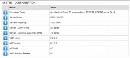
Figure 5-17 System configuration summary
Figure 5-18 shows the processor summary from the report. You can click any of the sections to retrieve an explanation of what the VIOS advisor is telling you, why it is important, and how to modify if there are problems detected.

Figure 5-18 Processor summary from the VIOS performance advisor
Figure 5-19 on page 274 shows the memory component of the VIOS Advisor report. If the VIOS performance advisor detects that more memory is to be added to the VIOS partition, it suggests the optimal amount of memory.
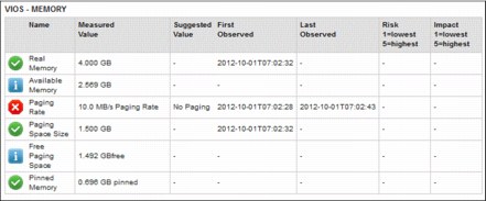
Figure 5-19 Memory summary
Figure 5-20 shows the disk and I/O summary. This shows the average amount of I/O and the block size being processed by the VIOS. It shows the amount of FC Adapters and their utilization.
|
Note: If the FC port speed is not optimal, it is possible that the FC adapter is attached to a SAN fabric switch that is either not capable of the speed of the FC adapter, or the switch ports are not configured correctly.
|
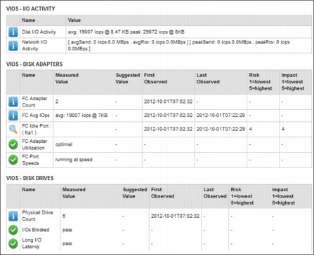
Figure 5-20 I/O and disk summary
If you click on the icon to the right of any item observed by the VIOS performance advisor, it provides a window, as shown in Figure 5-21 on page 275. This gives a more detailed description of what observation the VIOS performance advisor has made. The example shown in the figure shows an FC adapter that is unused, and the suggestion is to ensure that I/O is balanced across the available adapters. In an NPIV scenario, it could be that there are no LPARs mapped yet to this particular port.

Figure 5-21 Example of VIOS performance advisor recommendation
5.10 Workload management
One of the reasons why many systems have performance problems is because of poor workload distribution.
All planned activities can be better managed by following certain workload management techniques. This also helps to avoid bottleneck situations. There is work that can wait for a while. For instance, a report that needs to be generated for the next morning can be started at 5 p.m. or at 5 a.m. The difference is that during night the processor is probably idle. The critical data backup can also be initiated during the night to better manage the resources.
This type of workload management is provided by many different third-party software vendors, but the operating system itself has tools that may help before investing in such tools.
The cron daemon can be used to organize all planned workloads by running at different times. Use the at command to take advantage of the capability or set up a crontab file.
Using job queue is another way of workload management where the programs or procedures can be executed sequentially.
Submitting an environment for performance analysis is most of the time a complex task. It usually requires a good knowledge of the workloads running, system capacity, technologies available, and involves a lot of tuning and testing.
To understand the limits of the components of the environment is crucial for establishing targets and setting expectations.
Example 5-82 - qdaemon - configuration example
* BATCH queue for running shell scripts
bsh:
device = bshdev
discipline = fcfs
bshdev:
backend = /usr/bin/bsh
In Example 5-82 on page 275, we define a bsh queue that uses /usr/bin/bsh as backend. The backend is the program that is called by qdaemon.
The queue can be reduced by putting the jobs in the queue during the day and starting the queue up during the night using the commands shown in Example 5-83.
Example 5-83 - qdaemon - usage example
To bring the Queue down
# qadm -D bsh
To put the jobs in queue
# qprt -P bsh script1
# qprt -P bsh script2
# qprt -P bsh script3
To start the queue during night
# qadm -U bsh
When starting the queue during the night, the jobs will be executed sequentially.
Example 5-84 illustrates the use of queues to run a simple script with different behavior depending on the status of its control file. At first, ensure that the queue is down and some jobs are added to the queue. Next, the qchk output shows that our queue is down and has four jobs queued. When the queue is brought up, the jobs will run, all in sequence, sending output data to a log file. At last, with the queue still up, the job is submitted two more times. Check the timestamps of the log output.
Example 5-84 qdaemon - using the queue daemon to manage jobs
# qadm -D bsh
# qprt -P bsh /tests/job.sh
# qprt -P bsh /tests/job.sh
# qprt -P bsh /tests/job.sh
# qprt -P bsh /tests/job.sh
# qchk -P bsh
Queue Dev Status Job Files User PP % Blks Cp Rnk
------- ----- --------- --- ------------------ ---------- ---- -- ----- --- ---
bsh bshde DOWN
QUEUED 20 /tests/job.sh root 1 1 1
QUEUED 21 /tests/job.sh root 1 1 2
QUEUED 22 /tests/job.sh root 1 1 3
QUEUED 23 /tests/job.sh root 1 1 4
# qadm -U bsh
# qchk -P bsh
Queue Dev Status Job Files User PP % Blks Cp Rnk
------- ----- --------- --- ------------------ ---------- ---- -- ----- --- ---
bsh bshde READY
# cat /tmp/jobctl.log
[23/Oct/2012] - Phase: [prepare]
[23/Oct/2012] - Phase: [start]
[23/Oct/2012-18:24:49] - Phase: [finish]
Error
[23/Oct/2012-18:24:49] - Phase: []
[23/Oct/2012-18:24:49] - Phase: [prepare]
[23/Oct/2012-18:24:49] - Phase: [start]
[23/Oct/2012-18:27:38] - Creating reports.
[23/Oct/2012-18:27:38] - Error
[23/Oct/2012-18:27:38] - Preparing data.
[23/Oct/2012-18:27:38] - Processing data.
# qchk -P bsh
Queue Dev Status Job Files User PP % Blks Cp Rnk
------- ----- --------- --- ------------------ ---------- ---- -- ----- --- ---
bsh bshde READY
# qprt -P bsh /tests/job.sh
# qprt -P bsh /tests/job.sh
# tail -3 /tmp/jobctl.log
# tail -3 /tmp/jobctl.log
[23/Oct/2012-18:27:38] - Processing data.
[23/Oct/2012-18:28:03] - Creating reports.
[23/Oct/2012-18:33:38] - Error
Using this queueing technique to manage the workload can be useful to prevent some tasks running in parallel. For instance, it may be desired that the backups start only after all nightly reports are created. So instead of scheduling the reports and backup jobs with the cron daemon, you can use the queue approach and schedule only the queue startup within the crontab.
..................Content has been hidden....................
You can't read the all page of ebook, please click here login for view all page.