Depth- and Breadth-First Search

Before we look at higher-order analytical techniques we need to reacquaint ourselves with the fundamental breadth-first search algorithm, which is the basis for iterating over an entire graph. Most of the queries we’ve seen throughout this book have been depth-first rather than breadth-first in nature. That is, they traverse outward from a starting node to some end node before repeating a similar search down a different path from the same start node. Depth-first is a good strategy when we’re trying to follow a path to discover discrete pieces of information.

Though we’ve used depth-first search as our underlying strategy for general graph traversals, many interesting algorithms traverse the entire graph in a breadth-first manner. That is, they explore the graph one layer at a time, first visiting each node at depth 1 from the start node, then each of those at depth 2, then depth 3, and so on, until the entire graph has been visited. This progression is easily visualized starting at the node labeled O (for origin) and progressing outward a layer at a time, as shown in Figure 7-1.

Figure 7-1. The progression of a breadth-first search

Termination of the search depends on the algorithm being executed—most useful algorithms aren’t pure breadth-first search but are informed to some extent. Breadth-first search is often used in path-finding algorithms or when the entire graph needs to be systematically searched (for the likes of graph global algorithms we discussed in Chapter 3).

Path-Finding with Dijkstra’s Algorithm

Breadth-first search underpins numerous classical graph algorithms, including Dijkstra’s algorithm. Dijkstra (as it is often abbreviated) is used to find the shortest path between two nodes in a graph. Dijkstra’s algorithm is mature, having been published in 1956, and thereafter widely studied and optimized by computer scientists. It behaves as follows:

1. Pick the start and end nodes, and add the start node to the set of solved nodes (that is, the set of nodes with known shortest path from the start node) with value 0 (the start node is by definition 0 path length away from itself).

2. From the starting node, traverse breadth-first to the nearest neighbors and record the path length against each neighbor node.

3. Take the shortest path to one of these neighbors (picking arbitrarily in the case of ties) and mark that node as solved, because we now know the shortest path from the start node to this neighbor.

4. From the set of solved nodes, visit the nearest neighbors (notice the breath-first progression) and record the path lengths from the start node against these new neighbors. Don’t visit any neighboring nodes that have already been solved, because we know the shortest paths to them already.

5. Repeat steps 3 and 4 until the destination node has been marked solved.

Dijkstra is often used to find real-world shortest paths (e.g., for navigation). Here’s an example. In Figure 7-2 we see a logical map of Australia. Our challenge is to discover the shortest driving route between Sydney on the east coast (marked SYD) and Perth, marked PER, which is a continent away, on the west coast. The other major towns and cities are marked with their respective airport codes; we’ll discover many of them along the way.

Figure 7-2. A logical representation of Australia and its arterial road network

Starting at the node representing Sydney in Figure 7-3, we know the shortest path to Sydney is 0 hours, because we’re already there. In terms of Dijkstra’s algorithm, Sydney is now solved insofar as we know the shortest path from Sydney to Sydney. Accordingly, we’ve grayed out the node representing Sydney, added the path length (0), and thickened the node’s border—a convention that we’ll maintain throughout the remainder of this example.

Moving one level out from Sydney, our candidate cities are Brisbane, which lies to the north by 9 hours; Canberra, Australia’s capital city, which lies 4 hours to the west; and Melbourne, which is 12 hours to the south.

The shortest path we can find is Sydney to Canberra, at 4 hours, and so we consider Canberra to be solved, as shown in Figure 7-4.

Figure 7-3. The shortest path from Sydney to Sydney is unsurprisingly 0 hours

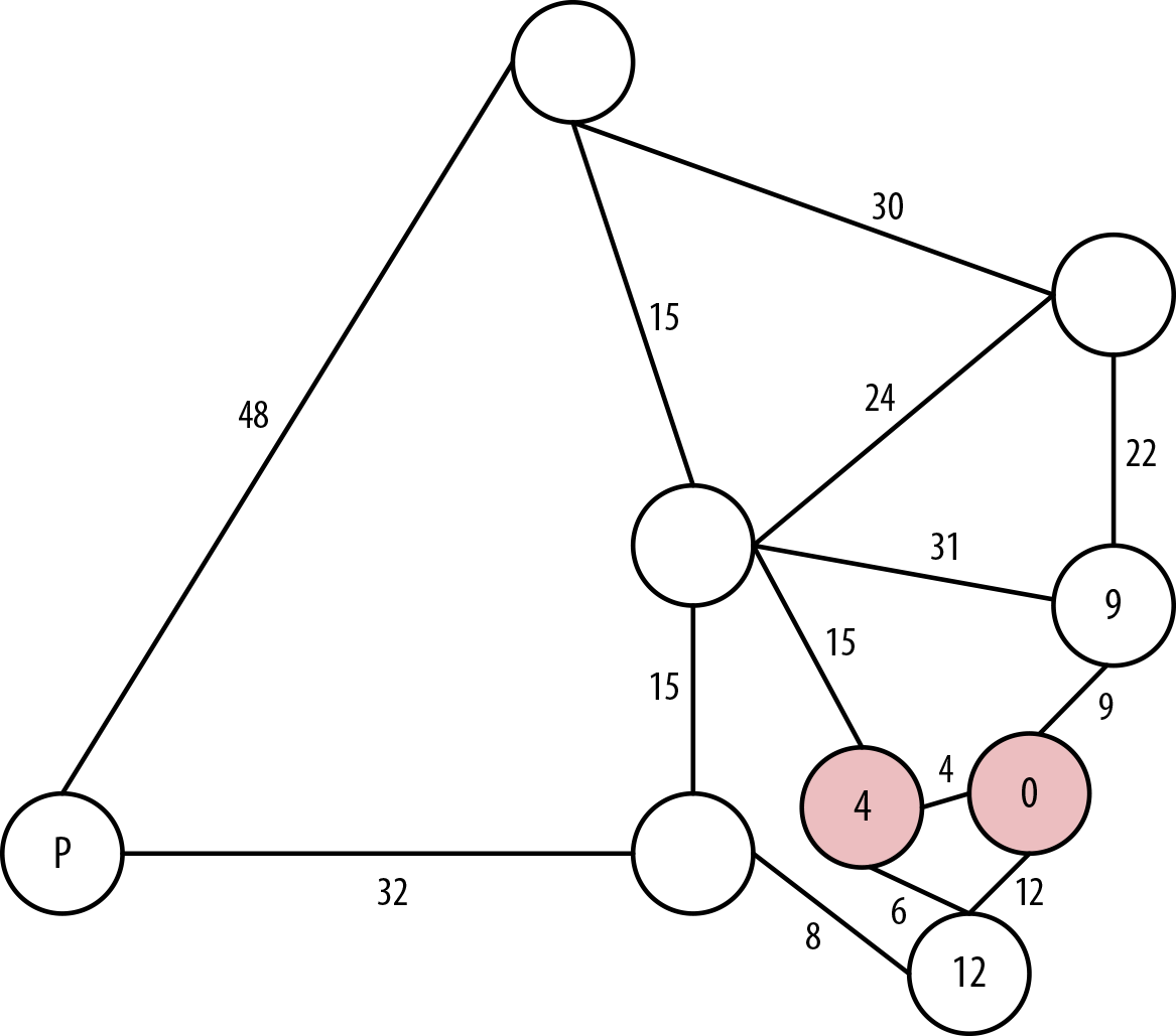
Figure 7-4. Canberra is the closest city to Sydney

The next nodes out from our solved nodes are Melbourne, at 10 hours from Sydney via Canberra, or 12 hours from Sydney directly, as we’ve already seen. We also have Alice Springs, which is 15 hours from Canberra and 19 hours from Sydney, or Brisbane, which is 9 hours direct from Sydney.

Accordingly, we explore the shortest path, which is 9 hours from Sydney to Brisbane, and consider Brisbane solved at 9 hours, as shown in Figure 7-5.

Figure 7-5. Brisbane is the next closest city

The next neighboring nodes from our solved ones are Melbourne, which is 10 hours via Canberra or 12 hours direct from Sydney along a different road; Cairns, which is 31 hours from Sydney via Brisbane; and Alice Springs, which is 40 hours via Brisbane or 19 hours via Canberra.

Accordingly, we choose the shortest path, which is Melbourne, being 10 hours from Sydney via Canberra. This is shorter than the existing 12 hours direct link. We now consider Melbourne solved, as shown in Figure 7-6.

Figure 7-6. Reaching Melbourne, the third-closest city to the start node of Sydney

In Figure 7-7, the next layer of neighboring nodes from our solved ones are Adelaide at 18 hours from Sydney (via Canberra and Melbourne); Cairns, at 31 hours from Sydney (via Brisbane); and Alice Springs, at 19 hours from Sydney via Canberra, or 40 hours via Brisbane. We choose Adelaide and consider it solved at a cost of 18 hours.

The next layer of neighboring nodes from our solved ones are Perth—our final destination—which is 50 hours from Sydney via Adelaide; Alice Springs, which is 19 hours from Sydney via Canberra or 33 hours via Adelaide; and Cairns, which is 31 hours from Sydney via Brisbane.

We choose Alice Springs in this case because it has the current shortest path, even though with a bird’s eye view we know that actually it’ll be shorter in the end to go from Adelaide to Perth—just ask any passing bushman. Our cost is 19 hours, as shown in Figure 7-8.

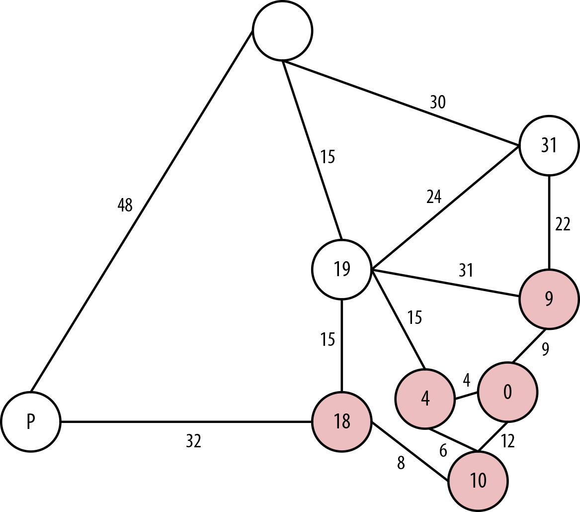
Figure 7-7. Solving Adelaide

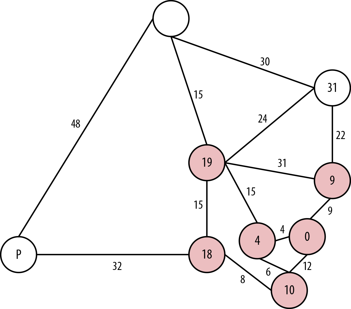
Figure 7-8. Taking a “detour” through Alice Springs

In Figure 7-9, the next layer of neighboring nodes from our solved ones are Cairns at 31 hours via Brisbane or 43 hours via Alice Springs, or Darwin at 34 hours via Alice Springs, or Perth via Adelaide at 50 hours. So we’ll take the route to Cairns via Brisbane and consider Cairns solved with a shortest driving time from Sydney at 31 hours.

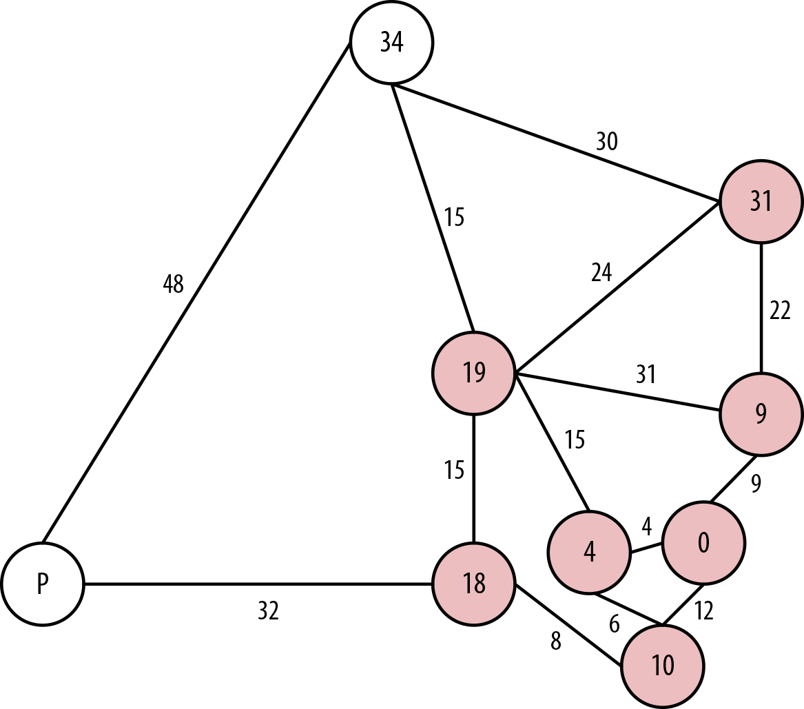
Figure 7-9. Back to Cairns on the east coast

The next layer of neighboring nodes from our solved ones are Darwin at 34 hours from Alice Springs, 61 hours via Cairns, or Perth via Adelaide at 50 hours. Accordingly, we choose the path to Darwin from Alice Springs at a cost of 34 hours and consider Darwin solved, as we can see in Figure 7-10.

Finally, the only neighboring node left is Perth itself, as we can see in Figure 7-11. It is accessible via Adelaide at a cost of 50 hours or via Darwin at a cost of 82 hours. Accordingly, we choose the route via Adelaide and consider Perth from Sydney solved at a shortest path of 50 hours.

Figure 7-10. To Darwin in Australia’s “top-end”

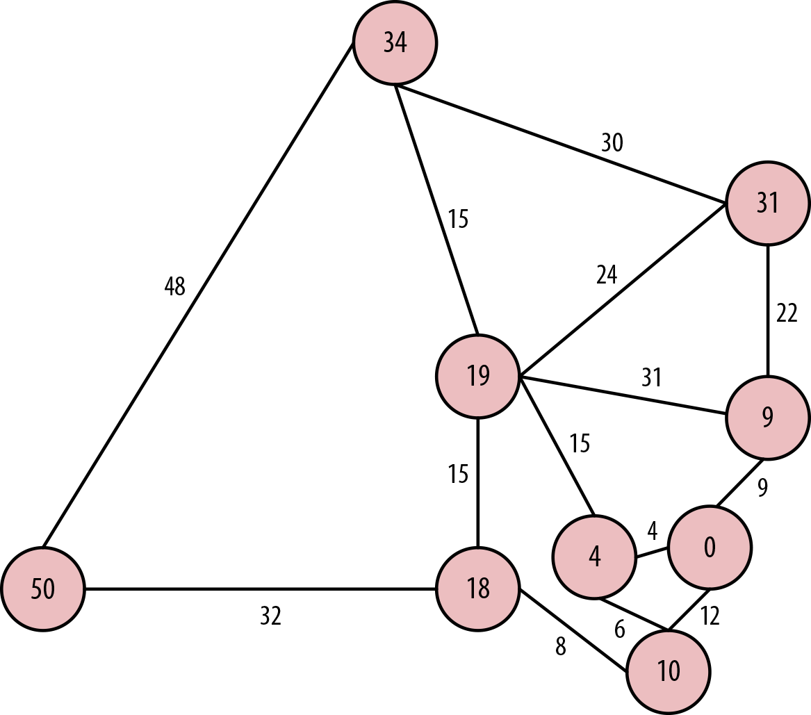
Figure 7-11. Finally reaching Perth, a mere 50 driving hours from Sydney

Dijkstra’s algorithm works well, but because its exploration is undirected, there are some pathological graph topologies that can cause worst-case performance problems. In these situations, we explore more of the graph than is intuitively necessary—in some cases, we explore the entire graph. Because each possible node is considered one at a time in relative isolation, the algorithm necessarily follows paths that intuitively will never contribute to the final shortest path.

Despite Dijkstra’s algorithm having successfully computed the shortest path between Sydney and Perth, anyone with any intuition about map reading would likely not have chosen to explore the route northward from Adelaide because it feels longer. If we had some heuristic mechanism to guide us, as in a best-first search (e.g., prefer to head west over east, prefer south over north) we might have avoided the side-trips to Brisbane, Cairns, Alice Springs, and Darwin in this example. But best-first searches are greedy, and try to move toward the destination node even if there is an obstacle (e.g., a dirt track) in the way. We can do better.

The A* Algorithm

The A* (pronounced “A-star”) algorithm improves on the classic Dijkstra algorithm. It is based on the observation that some searches are informed, and that by being informed we can make better choices over which paths to take through the graph. In our example, an informed search wouldn’t go from Sydney to Perth by traversing an entire continent to Darwin first. A* is like Dijkstra in that it can potentially search a large swathe of a graph, but it’s also like a greedy best-first search insofar as it uses a heuristic to guide it. A* combines aspects of Dijkstra’s algorithm, which prefers nodes close to the current starting point, and best-first search, which prefers nodes closer to the destination, to provide a provably optimal solution for finding shortest paths in a graph.

In A* we split the path cost into two parts: g(n), which is the cost of the path from the starting point to some node n; and h(n), which represents the estimated cost of the path from the node n to the destination node, as computed by a heuristic (an intelligent guess). The A* algorithm balances g(n) and h(n) as it iterates the graph, thereby ensuring that at each iteration it chooses the node with the lowest overall cost f(n) = g(n) + h(n).

As we’ve seen, breadth-first algorithms are particularly good for path finding. But they have other uses as well. Using breadth-first search as our method for iterating over all elements of a graph, we can now consider a number of interesting higher-order algorithms from graph theory that yield predictive insight into the behavior of connected data.

Graph Theory and Predictive Modeling

Graph theory is a mature and well-understood field of study concerning the nature of networks (or from our point of view, connected data). The analytic techniques that have been developed by graph theoreticians can be brought to bear on a range of interesting problems. Now that we understand the low-level traversal mechanisms, such as breadth-first search, we can start to consider higher-order analyses.

Graph theory techniques are broadly applicable to a wide range of problems. They are especially useful when we first want to gain some insight into a new domain—or even understand what kind of insight it’s possible to extract from a domain. In such cases there are a range of techniques from graph theory and social sciences that we can straightforwardly apply to gain insight.

In the next few sections we’ll introduce some of the key concepts in social graph theory. We’ll introduce these concepts in the context of a social domain based on the works of sociologists Mark Granovetter, and David Easley and Jon Kleinberg.¹

Triadic Closures

A triadic closure is a common property of social graphs, where we observe that if two nodes are connected via a path involving a third node, there is an increased likelihood that the two nodes will become directly connected at some point in the future. This is a familiar social occurrence. If we happen to be friends with two people who don’t know one another, there’s an increased chance that those two people will become direct friends at some point in the future. The very fact that we are friends with both of them gives each the means and the motive to become friends directly. That is, there’s an increased chance the two will meet one another through hanging around with us, and a good chance that if they do meet, they’ll trust one another based on their mutual trust in us and our friendship choices. The very fact of their both being our friend is an indicator that with respect to each other they may be socially similar.

From his analysis, Granovetter noted that a subgraph upholds the strong triadic closure property if it has a node A with strong relationships to two other nodes, B and C. B and C then have at least a weak, and potentially a strong, relationship between them. This is a bold assertion, and it won’t always hold for all subgraphs in a graph. Nonetheless, it is sufficiently commonplace, particularly in social networks, as to be a credible predictive indicator.

Let’s see how the strong triadic closure property works as a predictive aid in a workplace graph. We’ll start with a simple organizational hierarchy in which Alice manages Bob and Charlie, but where there are not yet any connections between her subordinates, as shown in Figure 7-12.

Figure 7-12. Alice manages Bob and Charlie

This is a rather strange situation for the workplace. After all, it’s unlikely that Bob and Charlie will be total strangers to one another. As shown in Figure 7-13, whether they’re high-level executives and therefore peers under Alice’s executive management or whether they’re assembly-line workers and therefore close colleagues under Alice acting as foreman, even informally we might expect Bob and Charlie to be somehow connected.

Figure 7-13. Bob and Charlie work together under Alice

Because Bob and Charlie both work with Alice, there’s a strong possibility they’re going to end up working together, as we see in Figure 7-13. This is consistent with the strong triadic closure property, which suggests that either Bob is a peer of Charlie (we’ll call this a weak relationship) or that Bob works with Charlie (which we’ll term a strong relationship). Adding a third WORKS_WITH or PEER_OF relationship between Bob and Charlie closes the triangle—hence the term triadic closure.

The empirical evidence from many domains, including sociology, public health, psychology, anthropology, and even technology (e.g., Facebook, Twitter, LinkedIn), suggests that the tendency toward triadic closure is real and substantial. This is consistent with anecdotal evidence and sentiment. But simple geometry isn’t all that’s at work here: the quality of the relationships involved in a graph also have a significant bearing on the formation of stable triadic closures.

Structural Balance

If we recall Figure 7-12, it’s intuitive to see how Bob and Charlie can become coworkers (or peers) under Alice’s management. For example purposes, we’re going to make an assumption that the MANAGES relationship is somewhat negative (after all, people don’t like getting bossed around) whereas the PEER_OF and WORKS_WITH relationship are positive (because people generally like their peers and the folks they work with).

We know from our previous discussion on the strong triadic closure principle that in Figure 7-12 where Alice MANAGES Bob and Charlie, a triadic closure should be formed. That is, in the absence of any other constraints, we would expect at least a PEER_OF, a WORKS_WITH, or even a MANAGES relationship between Bob and Charlie.

A similar tendency toward creating a triadic closure exists if Alice MANAGES Bob who in turn WORKS_WITH Charlie, as we can see in Figure 7-14. Anecdotally this rings true: if Bob and Charlie work together it makes sense for them to share a manager, especially if the organization seemingly allows Charlie to function without managerial supervision.

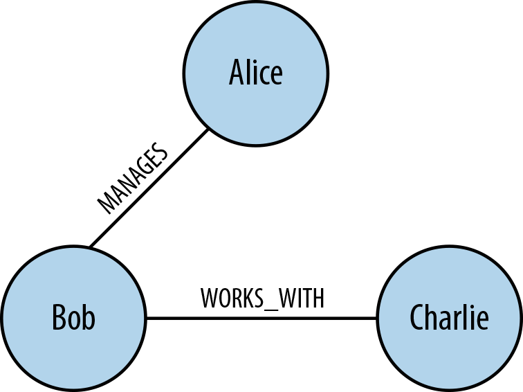
Figure 7-14. Alice manages Bob who works with Charlie

However, applying the strong triadic closure principle blindly can lead to some rather odd and uncomfortable-looking organization hierarchies. For instance, if Alice MANAGES Bob and Charlie but Bob also MANAGES Charlie, we have a recipe for discontent. Nobody would wish it upon Charlie that he’s managed both by his boss and his boss’s boss as in Figure 7-15.

Figure 7-15. Alice manages Bob and Charlie, while Bob also manages Charlie

Similarly, it’s uncomfortable for Bob if he is managed by Alice while working with Charlie who is also Alice’s workmate. This cuts awkwardly across organization layers as we see in Figure 7-16. It also means Bob could never safely let off steam about Alice’s management style amongst a supportive peer group.

Figure 7-16. Alice manages Bob who works with Charlie, while also working with Charlie

The awkward hierarchy in Figure 7-16 whereby Charlie is both a peer of the boss and a peer of another worker is unlikely to be socially pleasant, so Charlie and Alice will agitate against it (either wanting to be a boss or a worker). It’s similar for Bob who doesn’t know for sure whether to treat Charlie in the same way he treats his manager Alice (because Charlie and Alice are peers) or as his own direct peer.

It’s clear that the triadic closures in Figures 7-15 and 7-16 are uncomfortable to us, eschewing our innate preference for structural symmetry and rational layering. This preference is given a name in graph theory: structural balance.

Anecdotally, there’s a much more acceptable, structurally balanced triadic closure if Alice MANAGES Bob and Charlie, but where Bob and Charlie are themselves workmates connected by a WORKS_WITH relationship, as we can see in Figure 7-17.

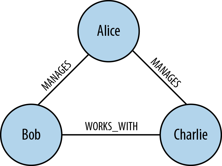
Figure 7-17. Workmates Bob and Charlie are managed by Alice

The same structural balance manifests itself in an equally acceptable triadic closure where Alice, Bob, and Charlie are all workmates. In this arrangement the workers are in it together, which can be a socially amicable arrangement that engenders camaraderie as in Figure 7-18.

Figure 7-18. Alice, Bob, and Charlie are all workmates

In Figures 7-17 and 7-18, the triadic closures are idiomatic and constructed with either three WORKS_WITH relationships or two MANAGES and a single WORKS_WITH relationship. They are all balanced triadic closures. To understand what it means to have balanced and unbalanced triadic closures, we’ll add more semantic richness to the model by declaring that the WORKS_WITH relationship is socially positive (because coworkers spend a lot of time interacting), whereas MANAGES is a negative relationship because managers spend overall less of their time interacting with individuals in their charge.

Given this new dimension of positive and negative sentiment, we can now ask the question “What is so special about these balanced structures?” It’s clear that strong triadic closure is still at work, but that’s not the only driver. In this case the notion of structural balance also has an effect. A structurally balanced triadic closure consists of relationships of all strong sentiments (our WORKS_WITH or PEER_OF relationships) or two relationships having negative sentiments (MANAGES in our case) with a single positive relationship.

We see this often in the real world. If we have two good friends, then social pressure tends toward those good friends themselves becoming good friends. It’s unusual that those two friends themselves are enemies because that puts a strain on all our friendships. One friend cannot express his dislike of the other to us, because the other person is our friend too! Given those pressures, it’s one outcome that the group will resolve its differences and good friends will emerge. This would change our unbalanced triadic closure (two relationships with positive sentiments and one negative) to a balanced closure because all relationships would be of a positive sentiment much like our collaborative scheme where Alice, Bob, and Charlie all work together in Figure 7-18.

However, the plausible (though arguably less pleasant) outcome would be where we take sides in the dispute between our “friends,” creating two relationships with negative sentiments—effectively ganging up on an individual. Now we can engage in gossip about our mutual dislike of a former friend and the closure again becomes balanced. Equally we see this reflected in the organizational scenario where Alice, by managing Bob and Charlie, becomes, in effect, their workplace enemy as in Figure 7-17.

Balanced closures add another dimension to the predictive power of graphs. Simply by looking for opportunities to create balanced closures across a graph, even at very large scale, we can modify the graph structure for accurate predictive analyses. But we can go further, and in the next section we’ll bring in the notion of local bridges, which give us valuable insight into the communications flow of our organization, and from that knowledge comes the ability to adapt it to meet future challenges.

Local Bridges

An organization of only three people as we’ve been using is anomalous, and the graphs we’ve studied in this section are best thought of as small subgraphs as part of a larger organizational hierarchy. When we start to consider managing a larger organization we expect a much more complex graph structure, but we can also apply other heuristics to the structure to help make sense of the business. In fact, once we have introduced other parts of the organization into the graph, we can reason about global properties of the graph based on the locally acting strong triadic closure principle.

In Figure 7-19, we’re presented with a counterintuitive scenario where two groups in the organization are managed by Alice and Davina, respectively. However, we have the slightly awkward structure that Alice not only runs a team with Bob and Charlie, but also manages Davina. Though this isn’t beyond the realm of possibility (Alice may indeed have such responsibilities), it feels intuitively awkward from an organizational design perspective.

Figure 7-19. Alice has skewed line management responsibility

From a graph theory perspective it’s also unlikely. Because Alice participates in two strong relationships, she MANAGES Charlie (and Bob) and MANAGES Davina, naturally we’d like to create a triadic closure by adding at least a PEER_OF relationship between Davina and Charlie (and Bob). But Alice is also involved in a local bridge to Davina—together they’re a sole communication path between groups in the organization. Having the relationship Alice MANAGES Davina means we’d in fact have to create the closure. These two properties—local bridge and strong triadic closure—are in opposition.

Yet if Alice and Davina are peers (a weak relationship), then the strong triadic closure principle isn’t activated because there’s only one strong relationship—the MANAGES relationship to Bob (or Charlie)—and the local bridge property is valid as we can see in Figure 7-20.

What’s interesting about this local bridge is that it describes a communication channel between groups in our organization. Such channels are extremely important to the vitality of our enterprise. In particular, to ensure the health of our company we’d make sure that local bridge relationships are healthy and active, or equally we might keep an eye on local bridges to ensure that no impropriety (embezzlement, fraud, etc.) occurs.

Figure 7-20. Alice and Davina are connected by a local bridge

This same property of local bridges being weak links (PEER_OF in our example organization) is a property that is prevalent throughout social graphs. This means we can start to make predictive analyses of how our organization will evolve based on empirically derived local bridge and strong triadic closure notions. So given an arbitrary organizational graph, we can see how the business structure is likely to evolve and plan for those eventualities.

Summary

Graphs are truly remarkable structures. Our understanding of them is rooted in hundreds of years of mathematical and scientific study. And yet we’re only just beginning to understand how to apply them to our personal, social, and business lives. The technology is here, open and available to all in the form of the modern graph database. The opportunities are endless.

As we’ve seen throughout this book, graph theory algorithms and analytical techniques are not demanding. We need only understand how to apply them to achieve our goals. We leave this book with a simple call to arms: embrace graphs and graph databases. Take all that you’ve learned about modeling with graphs, graph database architecture, designing and implementing a graph database solution, and applying graph algorithms to complex business problems, and go build the next truly pioneering information system.