
Chapter 4. Arrays, slices, and maps
In this chapter
- Array internals and fundamentals
- Managing collections of data with slices
- Working with key/value pairs using maps
It’s difficult to write programs that don’t need to store and read collections of data. If you use databases or files, or access the web, you need a way to handle the data you receive and send. Go has three different data structures that allow you to manage collections of data: arrays, slices, and maps. These data structures are baked into the language and used throughout the standard library. Once you learn how these data structures work, programming in Go will become fun, fast, and flexible.
4.1. Array internals and fundamentals
It makes sense to start with arrays because they form the base data structure for both slices and maps. Understanding how arrays work will help you appreciate the elegance and power that slices and maps provide.
4.1.1. Internals
An array in Go is a fixed-length data type that contains a contiguous block of elements of the same type. This could be a built-in type such as integers and strings, or it can be a struct type.
In figure 4.1 you can see the representation of an array. The elements of the array are marked as a grey box and are connected in series to each other. Each element contains the same type, in this case an integer, and can be accessed through a unique index position.
Figure 4.1. Array internals

Arrays are valuable data structures because the memory is allocated sequentially. Having memory in a contiguous form can help to keep the memory you use stay loaded within CPU caches longer. Using index arithmetic, you can iterate through all the elements of an array quickly. The type information for the array provides the distance in memory you have to move to find each element. Since each element is of the same type and follows each other sequentially, moving through the array is consistent and fast.
4.1.2. Declaring and initializing
An array is declared by specifying the type of data to be stored and the total number of elements required, also known as the array’s length.
Listing 4.1. Declaring an array set to its zero value
// Declare an integer array of five elements.
var array [5]int
Once an array is declared, neither the type of data being stored nor its length can be changed. If you need more elements, you need to create a new array with the length needed and then copy the values from one array to the other.
When variables in Go are declared, they’re always initialized to their zero value for their respective type, and arrays are no different. When an array is initialized, each individual element that belongs to the array is initialized to its zero value. In figure 4.2, you can see an array of integers with each element in the array initialized to 0, the zero value for integers.
Figure 4.2. Values of the array after the declaration of the array variable

A fast and easy way to create and initialize arrays is to use an array literal. Array literals allow you to declare the number of elements you need and specify values for those elements.
Listing 4.2. Declaring an array using an array literal
// Declare an integer array of five elements.
// Initialize each element with a specific value.
array := [5]int{10, 20, 30, 40, 50}
If the length is given as ..., Go will identify the length of the array based on the number of elements that are initialized.
Listing 4.3. Declaring an array with Go calculating size
// Declare an integer array.
// Initialize each element with a specific value.
// Capacity is determined based on the number of values initialized.
array := [...]int{10, 20, 30, 40, 50}
If you know the length of the array you need, but are only ready to initialize specific elements, you can use this syntax.
Listing 4.4. Declaring an array initializing specific elements
// Declare an integer array of five elements.
// Initialize index 1 and 2 with specific values.
// The rest of the elements contain their zero value.
array := [5]int{1: 10, 2: 20}
The values for the array declared in listing 4.4 will look like figure 4.3 after the array is declared and initialized.
Figure 4.3. Values of the array after the declaration of the array variable

4.1.3. Working with arrays
As we talked about, arrays are efficient data structures because the memory is laid out in sequence. This gives arrays the advantage of being efficient when accessing individual elements. To access an individual element, use the [ ] operator.
Listing 4.5. Accessing array elements
// Declare an integer array of five elements.
// Initialize each element with a specific value.
array := [5]int{10, 20, 30, 40, 50}

// Change the value at index 2.
array[2] = 35
The values for the array declared in listing 4.5 will look like figure 4.4 after the array operations are complete.
Figure 4.4. Values of the array after changing the value of index 2

You can have an array of pointers. Like in chapter 2, you use the * operator to access the value that each element pointer points to.
Listing 4.6. Accessing array pointer elements
// Declare an integer pointer array of five elements.
// Initialize index 0 and 1 of the array with integer pointers.
array := [5]*int{0: new(int), 1: new(int)}

// Assign values to index 0 and 1.
*array[0] = 10
*array[1] = 20
The values for the array declared in listing 4.6 will look like figure 4.5 after the array operations are complete.
Figure 4.5. An array of pointers that point to integers

An array is a value in Go. This means you can use it in an assignment operation. The variable name denotes the entire array and, therefore, an array can be assigned to other arrays of the same type.
Listing 4.7. Assigning one array to another of the same type
// Declare a string array of five elements.
var array1 [5]string

// Declare a second string array of five elements.
// Initialize the array with colors.
array2 := [5]string{"Red", "Blue", "Green", "Yellow", "Pink"}

// Copy the values from array2 into array1.
array1 = array2
After the copy, you have two arrays with identical values, as shown in figure 4.6.
Figure 4.6. Both arrays after the copy

The type of an array variable includes both the length and the type of data that can be stored in each element. Only arrays of the same type can be assigned.
Listing 4.8. Compiler error assigning arrays of different types
// Declare a string array of four elements.
var array1 [4]string

// Declare a second string array of five elements.
// Initialize the array with colors.
array2 := [5]string{"Red", "Blue", "Green", "Yellow", "Pink"}

// Copy the values from array2 into array1.
array1 = array2

Compiler Error:
cannot use array2 (type [5]string) as type [4]string in assignment
Copying an array of pointers copies the pointer values and not the values that the pointers are pointing to.
Listing 4.9. Assigning one array of pointers to another
// Declare a string pointer array of three elements.
var array1 [3]*string

// Declare a second string pointer array of three elements.
// Initialize the array with string pointers.
array2 := [3]*string{new(string), new(string), new(string)}

// Add colors to each element
*array2[0] = "Red"
*array2[1] = "Blue"
*array2[2] = "Green"

// Copy the values from array2 into array1.
array1 = array2
After the copy, you have two arrays pointing to the same strings, as shown in figure 4.7.
Figure 4.7. Two arrays of pointers that point to the same strings

4.1.4. Multidimensional arrays
Arrays are always one-dimensional, but they can be composed to create multidimensional arrays. Multidimensional arrays come in handy when you need to manage data that may have parent/child relationships or is associated with a coordinate system.
Listing 4.10. Declaring two-dimensional arrays
// Declare a two dimensional integer array of four elements
// by two elements.
var array [4][2]int

// Use an array literal to declare and initialize a two
// dimensional integer array.
array := [4][2]int{{10, 11}, {20, 21}, {30, 31}, {40, 41}}

// Declare and initialize index 1 and 3 of the outer array.
array := [4][2]int{1: {20, 21}, 3: {40, 41}}

// Declare and initialize individual elements of the outer
// and inner array.
array := [4][2]int{1: {0: 20}, 3: {1: 41}}
Figure 4.8 shows the values each array contains after declaring and initializing these arrays.
Figure 4.8. Two-dimensional arrays and their outer and inner values

To access an individual element, use the [ ] operator again and a bit of composition.
Listing 4.11. Accessing elements of a two-dimensional array
// Declare a two dimensional integer array of two elements.
var array [2][2]int

// Set integer values to each individual element.
array[0][0] = 10
array[0][1] = 20
array[1][0] = 30
array[1][1] = 40
You can copy multidimensional arrays into each other as long as they have the same type. The type of a multidimensional array is based on the length of each dimension and the type of data that can be stored in each element.
Listing 4.12. Assigning multidimensional arrays of the same type
// Declare two different two dimensional integer arrays.
var array1 [2][2]int
var array2 [2][2]int

// Add integer values to each individual element.
array2[0][0] = 10
array2[0][1] = 20
array2[1][0] = 30
array2[1][1] = 40

// Copy the values from array2 into array1.
array1 = array2
Because an array is a value, you can copy individual dimensions.
Listing 4.13. Assigning multidimensional arrays by index
// Copy index 1 of array1 into a new array of the same type.
var array3 [2]int = array1[1]

// Copy the integer found in index 1 of the outer array
// and index 0 of the interior array into a new variable of
// type integer.
var value int = array1[1][0]
4.1.5. Passing arrays between functions
Passing an array between functions can be an expensive operation in terms of memory and performance. When you pass variables between functions, they’re always passed by value. When your variable is an array, this means the entire array, regardless of its size, is copied and passed to the function.
To see this in action, let’s create an array of one million elements of type int. On a 64-bit architecture, this would require eight million bytes, or eight megabytes, of memory. What happens when you declare an array of that size and pass it to a function?
Listing 4.14. Passing a large array by value between functions
// Declare an array of 8 megabytes.
var array [1e6]int

// Pass the array to the function foo.
foo(array)

// Function foo accepts an array of one million integers.
func foo(array [1e6]int) {
    ...
}
Every time the function foo is called, eight megabytes of memory has to be allocated on the stack. Then the value of the array, all eight megabytes of memory, has to be copied into that allocation. Go can handle this copy operation, but there’s a better and more efficient way of doing this. You can pass a pointer to the array and only copy eight bytes, instead of eight megabytes of memory on the stack.
Listing 4.15. Passing a large array by pointer between functions
// Allocate an array of 8 megabytes.
var array [1e6]int

// Pass the address of the array to the function foo.
foo(&array)

// Function foo accepts a pointer to an array of one million integers.
func foo(array *[1e6]int) {
    ...
}
This time the function foo takes a pointer to an array of one million elements of type integer. The function call now passes the address of the array, which only requires eight bytes of memory to be allocated on the stack for the pointer variable.
This operation is much more efficient with memory and could yield better performance. You just need to be aware that because you’re now using a pointer, changing the value that the pointer points to will change the memory being shared. What is really awesome is that slices inherently take care of dealing with these types of issues, as you’ll see.
4.2. Slice internals and fundamentals
A slice is a data structure that provides a way for you to work with and manage collections of data. Slices are built around the concept of dynamic arrays that can grow and shrink as you see fit. They’re flexible in terms of growth because they have their own built-in function called append, which can grow a slice quickly with efficiency. You can also reduce the size of a slice by slicing out a part of the underlying memory. Slices give you all the benefits of indexing, iteration, and garbage collection optimizations because the underlying memory is allocated in contiguous blocks.
4.2.1. Internals
Slices are tiny objects that abstract and manipulate an underlying array. They’re three-field data structures that contain the metadata Go needs to manipulate the underlying arrays (see figure 4.9).
Figure 4.9. Slice internals with underlying array

The three fields are a pointer to the underlying array, the length or the number of elements the slice has access to, and the capacity or the number of elements the slice has available for growth. The difference between length and capacity will make more sense in a bit.
4.2.2. Creating and initializing
There are several ways to create and initialize slices in Go. Knowing the capacity you need ahead of time will usually determine how you go about creating your slice.
Make and slice literals
One way to create a slice is to use the built-in function make. When you use make, one option you have is to specify the length of the slice.
Listing 4.16. Declaring a slice of strings by length
// Create a slice of strings.
// Contains a length and capacity of 5 elements.
slice := make([]string, 5)
When you just specify the length, the capacity of the slice is the same. You can also specify the length and capacity separately.
Listing 4.17. Declaring a slice of integers by length and capacity
// Create a slice of integers.
// Contains a length of 3 and has a capacity of 5 elements.
slice := make([]int, 3, 5)
When you specify the length and capacity separately, you can create a slice with available capacity in the underlying array that you don’t have access to initially. Figure 4.9 depicts what the slice of integers declared in listing 4.17 could look like after it’s initialized with some values.
The slice in listing 4.17 has access to three elements, but the underlying array has five elements. The two elements not associated with the length of the slice can be incorporated so the slice can use those elements as well. New slices can also be created to share this same underlying array and use any existing capacity.
Trying to create a slice with a capacity that’s smaller than the length is not allowed.
Listing 4.18. Compiler error setting capacity less than length
// Create a slice of integers.
// Make the length larger than the capacity.
slice := make([]int, 5, 3)

Compiler Error:
len larger than cap in make([]int)
An idiomatic way of creating a slice is to use a slice literal. It’s similar to creating an array, except you don’t specify a value inside of the [ ] operator. The initial length and capacity will be based on the number of elements you initialize.
Listing 4.19. Declaring a slice with a slice literal
// Create a slice of strings.
// Contains a length and capacity of 5 elements.
slice := []string{"Red", "Blue", "Green", "Yellow", "Pink"}

// Create a slice of integers.
// Contains a length and capacity of 3 elements.
slice := []int{10, 20, 30}
When using a slice literal, you can set the initial length and capacity. All you need to do is initialize the index that represents the length and capacity you need. The following syntax will create a slice with a length and capacity of 100 elements.
Listing 4.20. Declaring a slice with index positions
// Create a slice of strings.
// Initialize the 100th element with an empty string.
slice := []string{99: ""}
Remember, if you specify a value inside the [ ] operator, you’re creating an array. If you don’t specify a value, you’re creating a slice.
Listing 4.21. Declaration differences between arrays and slices
// Create an array of three integers.
array := [3]int{10, 20, 30}

// Create a slice of integers with a length and capacity of three.
slice := []int{10, 20, 30}
nil and empty slices
Sometimes in your programs you may need to declare a nil slice. A nil slice is created by declaring a slice without any initialization.
Listing 4.22. Declaring a nil slice
// Create a nil slice of integers.
var slice []int
A nil slice is the most common way you create slices in Go. They can be used with many of the standard library and built-in functions that work with slices. They’re useful when you want to represent a slice that doesn’t exist, such as when an exception occurs in a function that returns a slice (see figure 4.10).
Figure 4.10. The representation of a nil slice

You can also create an empty slice by declaring a slice with initialization.
Listing 4.23. Declaring an empty slice
// Use make to create an empty slice of integers.
slice := make([]int, 0)

// Use a slice literal to create an empty slice of integers.
slice := []int{}
An empty slice contains a zero-element underlying array that allocates no storage. Empty slices are useful when you want to represent an empty collection, such as when a database query returns zero results (see figure 4.11).
Figure 4.11. The representation of an empty slice

Regardless of whether you’re using a nil slice or an empty slice, the built-in functions append, len, and cap work the same.
4.2.3. Working with slices
Now that you know what a slice is and how to create them, you can learn how to use them in your programs.
Assigning and slicing
Assigning a value to any specific index within a slice is identical to how you do this with arrays. To change the value of an individual element, use the [ ] operator.
Listing 4.24. Declaring an array using an array literal
// Create a slice of integers.
// Contains a length and capacity of 5 elements.
slice := []int{10, 20, 30, 40, 50}

// Change the value of index 1.
slice[1] = 25
Slices are called such because you can slice a portion of the underlying array to create a new slice.
Listing 4.25. Taking the slice of a slice
// Create a slice of integers.
// Contains a length and capacity of 5 elements.
slice := []int{10, 20, 30, 40, 50}


// Create a new slice.
// Contains a length of 2 and capacity of 4 elements.
newSlice := slice[1:3]
After the slicing operation performed in listing 4.25, we have two slices that are sharing the same underlying array. However, each slice views the underlying array in a different way (see figure 4.12).
Figure 4.12. Two slices sharing the same underlying array

The original slice views the underlying array as having a capacity of five elements, but the view of newSlice is different. For newSlice, the underlying array has a capacity of four elements. newSlice can’t access the elements of the underlying array that are prior to its pointer. As far as newSlice is concerned, those elements don’t even exist.
Calculating the length and capacity for any new slice is performed using the following formula.
Listing 4.26. How length and capacity are calculated
For slice[i:j] with an underlying array of capacity k

Length:   j - i
Capacity: k - i
If you apply this formula to newSlice you get the following.
Listing 4.27. Calculating the new length and capacity
For slice[1:3] with an underlying array of capacity 5

Length:   3 - 1 = 2
Capacity: 5 - 1 = 4
Another way to look at this is that the first value represents the starting index position of the element the new slice will start with—in this case, 1. The second value represents the starting index position (1) plus the number of elements you want to include (2); 1 plus 2 is 3, so the second value is 3. Capacity will be the total number of elements associated with the slice.
You need to remember that you now have two slices sharing the same underlying array. Changes made to the shared section of the underlying array by one slice can be seen by the other slice.
Listing 4.28. Potential consequence of making changes to a slice
// Create a slice of integers.
// Contains a length and capacity of 5 elements.
slice := []int{10, 20, 30, 40, 50}

// Create a new slice.
// Contains a length of 2 and capacity of 4 elements.
newSlice := slice[1:3]

// Change index 1 of newSlice.
// Change index 2 of the original slice.
newSlice[1] = 35
After the number 35 is assigned to the second element of newSlice, that change can also be seen by the original slice in element 3 (see figure 4.13).
Figure 4.13. The underlying array after the assignment operation

A slice can only access indexes up to its length. Trying to access an element outside of its length will cause a runtime exception. The elements associated with a slice’s capacity are only available for growth. They must be incorporated into the slice’s length before they can be used.
Listing 4.29. Runtime error showing index out of range
// Create a slice of integers.
// Contains a length and capacity of 5 elements.
slice := []int{10, 20, 30, 40, 50}

// Create a new slice.
// Contains a length of 2 and capacity of 4 elements.
newSlice := slice[1:3]

// Change index 3 of newSlice.
// This element does not exist for newSlice.
newSlice[3] = 45

Runtime Exception:
panic: runtime error: index out of range
Having capacity is great, but useless if you can’t incorporate it into your slice’s length. Luckily, Go makes this easy when you use the built-in function append.
Growing slices
One of the advantages of using a slice over using an array is that you can grow the capacity of your slice as needed. Go takes care of all the operational details when you use the built-in function append.
To use append, you need a source slice and a value that is to be appended. When your append call returns, it provides you a new slice with the changes. The append function will always increase the length of the new slice. The capacity, on the other hand, may or may not be affected, depending on the available capacity of the source slice.
Listing 4.30. Using append to add an element to a slice
// Create a slice of integers.
// Contains a length and capacity of 5 elements.
slice := []int{10, 20, 30, 40, 50}

// Create a new slice.
// Contains a length of 2 and capacity of 4 elements.
newSlice := slice[1:3]

// Allocate a new element from capacity.
// Assign the value of 60 to the new element.
newSlice = append(newSlice, 60)
After the append operation in listing 4.30, the slices and the underlying array will look like figure 4.14.
Figure 4.14. The underlying array after the append operation

Because there was available capacity in the underlying array for newSlice, the append operation incorporated the available element into the slice’s length and assigned the value. Since the original slice is sharing the underlying array, slice also sees the changes in index 3.
When there’s no available capacity in the underlying array for a slice, the append function will create a new underlying array, copy the existing values that are being referenced, and assign the new value.
Listing 4.31. Using append to increase the length and capacity of a slice
// Create a slice of integers.
// Contains a length and capacity of 4 elements.
slice := []int{10, 20, 30, 40}

// Append a new value to the slice.
// Assign the value of 50 to the new element.
newSlice := append(slice, 50)
After this append operation, newSlice is given its own underlying array, and the capacity of the array is doubled from its original size (see figure 4.15).
Figure 4.15. The new underlying array after the append operation

The append operation is clever when growing the capacity of the underlying array. Capacity is always doubled when the existing capacity of the slice is under 1,000 elements. Once the number of elements goes over 1,000, the capacity is grown by a factor of 1.25, or 25%. This growth algorithm may change in the language over time.
Three index slices
There’s a third index option we haven’t mentioned yet that you can use when you’re slicing. This third index gives you control over the capacity of the new slice. The purpose is not to increase capacity, but to restrict the capacity. As you’ll see, being able to restrict the capacity of a new slice provides a level of protection to the underlying array and gives you more control over append operations.
Let’s start with a slice of five strings that contain fruit you can find in your local supermarket.
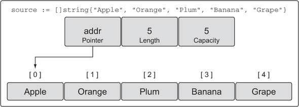
Listing 4.32. Declaring a slice of string using a slice literal
// Create a slice of strings.
// Contains a length and capacity of 5 elements.
source := []string{"Apple", "Orange", "Plum", "Banana", "Grape"}
If you inspect the values for this slice of fruit, it will look something like figure 4.16.
Figure 4.16. A representation of the slice of strings
Now let’s use the third index option to perform a slicing operation.
Listing 4.33. Performing a three-index slice
// Slice the third element and restrict the capacity.
// Contains a length of 1 element and capacity of 2 elements.
slice := source[2:3:4]
After this slicing operation, we have a new slice that references one element from the underlying array and has a capacity of two elements. Specifically, the new slice references the Plum element and has capacity up to the Banana element, as shown in figure 4.17.
Figure 4.17. A representation of the new slice after the operation

We can apply the same formula that we defined before to calculate the new slice’s length and capacity.
Listing 4.34. How length and capacity are calculated
For slice[i:j:k]  or  [2:3:4]

Length:   j - i  or  3 - 2 = 1
Capacity: k - i  or  4 - 2 = 2
Again, the first value represents the starting index position of the element the new slice will start with—in this case, 2. The second value represents the starting index position (2) plus the number of elements you want to include (1); 2 plus 1 is 3, so the second value is 3. For setting capacity, you take the starting index position of 2, plus the number of elements you want to include in the capacity (2), and you get the value of 4.
If you attempt to set a capacity that’s larger than the available capacity, you’ll get a runtime error.
Listing 4.35. Runtime error setting capacity larger than existing capacity
// This slicing operation attempts to set the capacity to 4.
// This is greater than what is available.
slice := source[2:3:6]

Runtime Error:
panic: runtime error: slice bounds out of range
As we’ve discussed, the built-in function append will use any available capacity first. Once that capacity is reached, it will allocate a new underlying array. It’s easy to forget which slices are sharing the same underlying array. When this happens, making changes to a slice can result in random and odd-looking bugs. Suddenly changes appear on multiple slices out of nowhere.
By having the option to set the capacity of a new slice to be the same as the length, you can force the first append operation to detach the new slice from the underlying array. Detaching the new slice from its original source array makes it safe to change.
Listing 4.36. Benefits of setting length and capacity to be the same
// Create a slice of strings.
// Contains a length and capacity of 5 elements.
source := []string{"Apple", "Orange", "Plum", "Banana", "Grape"}

// Slice the third element and restrict the capacity.
// Contains a length and capacity of 1 element.
slice := source[2:3:3]

// Append a new string to the slice.
slice = append(slice, "Kiwi")
Without this third index, appending Kiwi to our slice would’ve changed the value of Banana in index 3 of the underlying array, because all of the remaining capacity would still belong to the slice. But in listing 4.36, we restricted the capacity of the slice to 1. When we call append for the first time on the slice, it will create a new underlying array of two elements, copy the fruit Plum, add the new fruit Kiwi, and return a new slice that references this underlying array, as in figure 4.18.
Figure 4.18. A representation of the new slice after the append operation

With the new slice now having its own underlying array, we’ve avoided potential problems. We can now continue to append fruit to our new slice without worrying if we’re changing fruit to other slices inappropriately. Also, allocating the new underlying array for the slice was easy and clean.
The built-in function append is also a variadic function. This means you can pass multiple values to be appended in a single slice call. If you use the ... operator, you can append all the elements of one slice into another.
Listing 4.37. Appending to a slice from another slice
// Create two slices each initialized with two integers.
s1 := []int{1, 2}
s2 := []int{3, 4}

// Append the two slices together and display the results.
fmt.Printf("%v
", append(s1, s2...))

Output:
[1 2 3 4]
As you can see by the output, all the values of slice s2 have been appended to slice s1. The value of the new slice returned by the append function is then displayed by the call to Printf.
Iterating over slices
Since a slice is a collection, you can iterate over the elements. Go has a special keyword called range that you use in conjunction with the keyword for to iterate over slices.
Listing 4.38. Iterating over a slice using for range
// Create a slice of integers.
// Contains a length and capacity of 4 elements.
slice := []int{10, 20, 30, 40}

// Iterate over each element and display each value.
for index, value := range slice {
  fmt.Printf("Index: %d  Value: %d
", index, value)
}


Output:
Index: 0  Value: 10
Index: 1  Value: 20
Index: 2  Value: 30
Index: 3  Value: 40
The keyword range, when iterating over a slice, will return two values. The first value is the index position and the second value is a copy of the value in that index position (see figure 4.19).
Figure 4.19. Using range to iterate over a slice creates a copy of each element.

It’s important to know that range is making a copy of the value, not returning a reference. If you use the address of the value variable as a pointer to each element, you’ll be making a mistake. Let’s see why.
Listing 4.39. range provides a copy of each element
// Create a slice of integers.
// Contains a length and capacity of 4 elements.
slice := []int{10, 20, 30, 40}

// Iterate over each element and display the value and addresses.
for index, value := range slice {
   fmt.Printf("Value: %d  Value-Addr: %X  ElemAddr: %X
",
       value, &value, &slice[index])
}

Output:
Value: 10  Value-Addr: 10500168  ElemAddr: 1052E100
Value: 20  Value-Addr: 10500168  ElemAddr: 1052E104
Value: 30  Value-Addr: 10500168  ElemAddr: 1052E108
Value: 40  Value-Addr: 10500168  ElemAddr: 1052E10C
The address for the value variable is always the same because it’s a variable that contains a copy. The address of each individual element can be captured using the slice variable and the index value.
If you don’t need the index value, you can use the underscore character to discard the value.
Listing 4.40. Using the blank identifier to ignore the index value
// Create a slice of integers.
// Contains a length and capacity of 4 elements.
slice := []int{10, 20, 30, 40}

// Iterate over each element and display each value.
for _, value := range slice {
    fmt.Printf("Value: %d
", value)
}

Output:
Value: 10
Value: 20
Value: 30
Value: 40
The keyword range will always start iterating over a slice from the beginning. If you need more control iterating over a slice, you can always use a traditional for loop.
Listing 4.41. Iterating over a slice using a traditional for loop
// Create a slice of integers.
// Contains a length and capacity of 4 elements.
slice := []int{10, 20, 30, 40}

// Iterate over each element starting at element 3.
for index := 2; index < len(slice); index++ {
    fmt.Printf("Index: %d  Value: %d
", index, slice[index])
}

Output:
Index: 2  Value: 30
Index: 3  Value: 40
There are two special built-in functions called len and cap that work with arrays, slices, and channels. For slices, the len function returns the length of the slice, and the cap function returns the capacity. In listing 4.41, we used the len function to determine when to stop iterating over the slice.
Now that you know how to create and work with slices, you can use them to compose and iterate over multidimensional slices.
4.2.4. Multidimensional slices
Like arrays, slices are one-dimensional, but they can be composed to create multidimensional slices for the same reasons we discussed earlier.
Listing 4.42. Declaring a multidimensional slice
// Create a slice of a slice of integers.
slice := [][]int{{10}, {100, 200}}
We now have an outer slice of two elements that contain an inner slice of integers. The values for our slice of a slice of integers will look like figure 4.20.
Figure 4.20. Values for our slice of a slice of integers

In figure 4.20 you can see how composition is working to embed slices into slices. The outer slice contains two elements, each of which are slices. The slice in the first element is initialized with the single integer 10 and the slice in the second element contains two integers, 100 and 200.
Composition allows you to create very complex and powerful data structures. All of the rules you learned about the built-in function append still apply.
Listing 4.43. Composing slices of slices
// Create a slice of a slice of integers.
slice := [][]int{{10}, {100, 200}}

// Append the value of 20 to the first slice of integers.
slice[0] = append(slice[0], 20)
The append function and Go are elegant in how they handle growing and assigning the new slice of integers back into the first element of the outer slice. When the operation in listing 4.43 is complete, an entire new slice of integers and a new underlying array is allocated and then copied back into index 0 of the outer slice, as shown in figure 4.21.
Figure 4.21. What index 0 of the outer slice looks like after the append operation

Even with this simple multidimensional slice, there are a lot of layers and values involved. Passing a data structure like this between functions could seem complicated. But slices are cheap and passing them between functions is trivial.
4.2.5. Passing slices between functions
Passing a slice between two functions requires nothing more than passing the slice by value. Since the size of a slice is small, it’s cheap to copy and pass between functions. Let’s create a large slice and pass that slice by value to our function called foo.
Listing 4.44. Passing slices between functions
// Allocate a slice of 1 million integers.
slice := make([]int, 1e6)

// Pass the slice to the function foo.
slice = foo(slice)

// Function foo accepts a slice of integers and returns the slice back.
func foo(slice []int) []int {
    ...
    return slice
}
On a 64-bit architecture, a slice requires 24 bytes of memory. The pointer field requires 8 bytes, and the length and capacity fields require 8 bytes respectively. Since the data associated with a slice is contained in the underlying array, there are no problems passing a copy of a slice to any function. Only the slice is being copied, not the underlying array (see figure 4.22).
Figure 4.22. Both slices pointing to the underlying array after the function call

Passing the 24 bytes between functions is fast and easy. This is the beauty of slices. You don’t need to pass pointers around and deal with complicated syntax. You just create copies of your slices, make the changes you need, and then pass a new copy back.
4.3. Map internals and fundamentals
A map is a data structure that provides you with an unordered collection of key/value pairs.
You store values into the map based on a key. Figure 4.23 shows an example of a key/value pair you may store in your maps. The strength of a map is its ability to retrieve data quickly based on the key. A key works like an index, pointing to the value you associate with that key.
Figure 4.23. Relationship of key/value pairs

4.3.1. Internals
Maps are collections, and you can iterate over them just like you do with arrays and slices. But maps are unordered collections, and there’s no way to predict the order in which the key/value pairs will be returned. Even if you store your key/value pairs in the same order, every iteration over a map could return a different order. This is because a map is implemented using a hash table, as shown in figure 4.24.
Figure 4.24. Simple representation of the internal structure of a map

The map’s hash table contains a collection of buckets. When you’re storing, removing, or looking up a key/value pair, everything starts with selecting a bucket. This is performed by passing the key—specified in your map operation—to the map’s hash function. The purpose of the hash function is to generate an index that evenly distributes key/value pairs across all available buckets.
The better the distribution, the quicker you can find your key/value pairs as the map grows. If you store 10,000 items in your map, you don’t want to ever look at 10,000 key/value pairs to find the one you want. You want to look at the least number of key/value pairs possible. Looking at only 8 key/value pairs in a map of 10,000 items is a good and balanced map. A balanced list of key/value pairs across the right number of buckets makes this possible.
The hash key that’s generated for a Go map is a bit longer than what you see in figure 4.25, but it works the same way. In our example, the keys are strings that represents a color. Those strings are converted into a numeric value within the scope of the number of buckets we have available for storage. The numeric value is then used to select a bucket for storing or finding the specific key/value pair. In the case of a Go map, a portion of the generated hash key, specifically the low order bits (LOB), is used to select the bucket.
Figure 4.25. Simple view of how hash functions work

If you look at figure 4.24 again, you can see what the internals of a bucket look like. There are two data structures that contain the data for the map. First, there’s an array with the top eight high order bits (HOB) from the same hash key that was used to select the bucket. This array distinguishes each individual key/value pair stored in the respective bucket. Second, there’s an array of bytes that stores the key/value pairs. The byte array packs all the keys and then all the values together for the respective bucket. The packing of the key/value pairs is implemented to minimize the memory required for each bucket.
There are a lot of other low-level implementation details about maps that are outside the scope of this chapter. You don’t need to understand all the internals to learn how to create and use maps. Just remember one thing: a map is an unordered collection of key/value pairs.
4.3.2. Creating and initializing
There are several ways you can create and initialize maps in Go. You can use the built-in function make, or you can use a map literal.
Listing 4.45. Declaring a map using make
// Create a map with a key of type string and a value of type int.
dict := make(map[string]int)

// Create a map with a key and value of type string.
// Initialize the map with 2 key/value pairs.
dict := map[string]string{"Red": "#da1337", "Orange": "#e95a22"}
Using a map literal is the idiomatic way of creating a map. The initial length will be based on the number of key/value pairs you specify during initialization.
The map key can be a value from any built-in or struct type as long as the value can be used in an expression with the == operator. Slices, functions, and struct types that contain slices can’t be used as map keys. This will produce a compiler error.
Listing 4.46. Declaring an empty map using a map literal
// Create a map using a slice of strings as the key.
dict := map[[]string]int{}

Compiler Exception:
invalid map key type []string
There’s nothing stopping you from using a slice as a map value. This can come in handy when you need a single map key to be associated with a collection of data.
Listing 4.47. Declaring a map that stores slices of strings
// Create a map using a slice of strings as the value.
dict := map[int][]string{}
4.3.3. Working with maps
Assigning a key/value pair to a map is performed by specifying a key of the proper type and assigning a value to that key.
Listing 4.48. Assigning values to a map
// Create an empty map to store colors and their color codes.
colors := map[string]string{}

// Add the Red color code to the map.
colors["Red"] = "#da1337"
You can create a nil map by declaring a map without any initialization. A nil map can’t be used to store key/value pairs. Trying will produce a runtime error.
Listing 4.49. Runtime error assigned to a nil map
// Create a nil map by just declaring the map.
var colors map[string]string

// Add the Red color code to the map.
colors["Red"] = "#da1337"

Runtime Error:
panic: runtime error: assignment to entry in nil map
Testing if a map key exists is an important part of working with maps. It allows you to write logic that can determine if you’ve performed an operation or if you’ve cached some particular data in the map. It can also be used to compare two maps to identify what key/value pairs match or are missing.
When retrieving a value from a map, you have two choices. You can retrieve the value and a flag that explicitly lets you know if the key exists.
Listing 4.50. Retrieving a value from a map and testing existence.
// Retrieve the value for the key "Blue".
value, exists := colors["Blue"]

// Did this key exist?
if exists {
    fmt.Println(value)
}
The other option is to just return the value and test for the zero value to determine if the key exists. This will only work if the zero value is not a valid value for the map.
Listing 4.51. Retrieving a value from a map testing the value for existence
// Retrieve the value for the key "Blue".
value := colors["Blue"]

// Did this key exist?
if value != "" {
    fmt.Println(value)
}
When you index a map in Go, it will always return a value, even when the key doesn’t exist. In this case, the zero value for the value’s type is returned.
Iterating over a map is identical to iterating over an array or slice. You use the keyword range; but when it comes to maps, you don’t get back the index/value, you get back the key/value pairs.
Listing 4.52. Iterating over a map using for range
// Create a map of colors and color hex codes.
colors := map[string]string{
    "AliceBlue":   "#f0f8ff",
    "Coral":       "#ff7F50",
    "DarkGray":    "#a9a9a9",
    "ForestGreen": "#228b22",
}

// Display all the colors in the map.
for key, value := range colors {
    fmt.Printf("Key: %s  Value: %s
", key, value)
}
If you want to remove a key/value pair from the map, you use the built-in function delete.
Listing 4.53. Removing an item from a map
// Remove the key/value pair for the key "Coral".
delete(colors, "Coral")

// Display all the colors in the map.

for key, value := range colors {
    fmt.Printf("Key: %s  Value: %s
", key, value)
}
This time when you iterate through the map, the color Coral would not be displayed on the screen.
4.3.4. Passing maps between functions
Passing a map between two functions doesn’t make a copy of the map. In fact, you can pass a map to a function and make changes to the map, and the changes will be reflected by all references to the map.
Listing 4.54. Passing maps between functions
func main() {
    // Create a map of colors and color hex codes.
    colors := map[string]string{
       "AliceBlue":   "#f0f8ff",
       "Coral":       "#ff7F50",
       "DarkGray":    "#a9a9a9",
       "ForestGreen": "#228b22",
    }

    // Display all the colors in the map.
    for key, value := range colors {
        fmt.Printf("Key: %s  Value: %s
", key, value)
    }

    // Call the function to remove the specified key.
    removeColor(colors, "Coral")

    // Display all the colors in the map.
    for key, value := range colors {
        fmt.Printf("Key: %s  Value: %s
", key, value)
    }
}

// removeColor removes keys from the specified map.
func removeColor(colors map[string]string, key string) {
    delete(colors, key)
}
If you run this program, you’ll get the following output.
Listing 4.55. Output for listing 4.54
Key: AliceBlue Value: #F0F8FF
Key: Coral Value: #FF7F50
Key: DarkGray Value: #A9A9A9
Key: ForestGreen Value: #228B22

Key: AliceBlue Value: #F0F8FF
Key: DarkGray Value: #A9A9A9
Key: ForestGreen Value: #228B22
You can see that after the call to removeColor is complete, the color Coral is no longer present in the map referenced by main. Maps are designed to be cheap, similar to slices.
4.4. Summary
- Arrays are the building blocks for both slices and maps.
- Slices are the idiomatic way in Go you work with collections of data. Maps are the way you work with key/value pairs of data.
- The built-in function make allows you to create slices and maps with initial length and capacity. Slice and map literals can be used as well and support setting initial values for use.
- Slices have a capacity restriction, but can be extended using the built-in function append.
- Maps don’t have a capacity or any restriction on growth.
- The built-in function len can be used to retrieve the length of a slice or map.
- The built-in function cap only works on slices.
- Through the use of composition, you can create multidimensional arrays and slices. You can also create maps with values that are slices and other maps. A slice can’t be used as a map key.
- Passing a slice or map to a function is cheap and doesn’t make a copy of the underlying data structure.