12
Portland
Risk and Vulnerability Assessment
12.1 Introduction
Risks and vulnerabilities exist throughout every city. These risks and vulnerabilities have to be prioritized based on their consequence and frequency to decide best how to decrease the effects on the city. Critical assets throughout the city must also be identified and prioritized so that concerns for attacks on those assets can be managed. Risks in cities can also relate to emissions released by certain activities across the city. Most risks in a city can be controlled or brought down to a more tolerable effect. Several assessments can be performed, including rapid risk assessment (RRA), vulnerability assessment (VA), and integrated regional risk assessment (IRRA) to determine the most critical risks to a city. When developing a comprehensive implementation plan to solve a problem, it is essential to account for resiliency. This will allow for a developed system, or solution, capable of preventing and mitigating risks and recovering from failures. In these a ReIDMP can be helpful. This chapter aims to illustrate how the ReIDMP can be combined with readily available manuals, guidelines, assessments, and tools to better understand a city in terms of risks and vulnerabilities to mitigate their effects in a realistic case. To achieve this aim, this chapter is organized as follows: First, it articulates ten different risks in the selected city, Portland, Oregon (USA), using the RRA methodologies from Manual for the Classification of Prioritization of Risks Due to Major Accidents in Process and Related Industries (International Atomic Energy Agency 1996). Vulnerability of certain critical assets along transportation routes is then conducted using the VA methodologies from Guide to Highway Vulnerability Assessment for Critical Asset Identification and Protection (Science Applications International Corporation 2002). Air, water, and soil emissions analyses are then conducted throughout the city, and the effects on citizens in the area are addressed using the IRRA methodologies from Guidelines for Integrated Risk Assessment and Management in Large Industrial Areas (International Atomic Energy Agency 1998). The effects of electromagnetic pulse (EMP) blasts at varying heights above a city are suggested. Finally, a ReIDMP for Portland is then provided to indicate the transportability of the model. Unless otherwise noted, Google Earth Pro v.7.3.4. (https://earth.google.com) is used to visualize the city.
In this realistic case, the actual City of Portland, is impacted by fixed risks and the transportation of hazardous goods. In addition, many of the city’s critical assets are susceptible to attacks, and the city houses many sources of continuous emissions. All these aspects increase risks throughout the city and endanger the health and safety of those living in and visiting the city. City officials would like various assessments to be completed to identify risks and vulnerabilities throughout the city to make the city safer for those in and around the city. Due to budgets, city officials are looking for prioritized lists of risks and vulnerabilities. Multiple assessments, including the RRA, VA, IRRA, and EMP, will be completed to assist with the requests of the city officials. In addition, the city officials request a ReIDMP model to assist with developing resilient systems. After completing these assessments, city officials hope to make Portland a safe place for its citizens and visitors. A short, concise problem statement for this issue can be written as follows:
The city of Portland, OR is experiencing high levels of risk and vulnerability throughout the city. This issue is affecting the safety and health of hundreds-of-thousands citizens and visitors in and around the city as evidenced by observations, studies, and assessments.
12.2 Rapid Risk Assessment
RRA aims to identify possible risks throughout a specified area, determine the consequence and frequency of each risk, and prioritize each risk. The Manual for the Classification of Prioritization of Risks Due to Major Accidents in Process and Related Industries (International Atomic Energy Agency 1996) is used to perform the RRA for the chosen area of Portland. This manual includes detailed instructions for each step, which are discussed and summarized throughout this section. Figure 12.1 depicts the selected analysis area in Google Earth Pro v.7.3.4.

Figure 12.1 The selected analysis area of Portland.
RRA consists of five main steps: (i) classification of type of activities and inventories, (ii) estimation of consequences, (iii) estimation of probabilities, (iv) estimation of social risks, and (v) prioritization of risks. The risks evaluated in this assessment include both fixed installations and the transportation of hazardous goods.
12.2.1 Classification of Types of Activities and Inventories
A total of ten risks are assessed. Each risk, the type of risk, and its associated substances causing risk are listed in Table 12.1. Figure 12.2 depicts the location of risks throughout the city.

Figure 12.2 The location of risks.
Table 12.1 Risks in Portland and the associated substances.
| Risk | Associated substance | Type |
|---|---|---|
| Ice rink | Ammonia | Fixed |
| Bus garage | Petrol | Fixed |
| Competition pool | Chlorine | Fixed |
| Forge | Carbon monoxide | Fixed |
| Pest control service | Phosgene | Fixed |
| Sugar refinery | Sulfur dioxide | Fixed |
| Composite wood manufacturer | Formaldehyde | Fixed |
| Gas distribution center | Petrol | Fixed |
| Gas transportation | Petrol | Transportation |
| Chlorine transportation | Chlorine | Transportation |
12.2.2 Estimation of Consequences
Step 2 involves estimating the consequence of each risk event. Equation (12.1) is used to assess consequences.
where:
A = affected area (ha)
δ = population density in a defined populated area (persons/ha)
fA = correction factor for the populated area (part of circle)
fd = correction factor for the populated area (distances)
fm = correction factor for mitigation effects
Using this equation allows you to solve for Ca,s, which is the number of consequences (number of fatalities/accident) of an accident caused by the substance (subscript s) for each identified activity (subscript a). The consequence for each risk will be detailed in Sections 12.2.3–12.2.6.
12.2.3 Estimation of Probabilities
Step 3 is the estimation of the probability, or frequency, of each risk for both fixed installations and transportation risks. To calculate the frequency (Pi,s, number of accidents per year) of accidents involving a hazardous substance (subscript s) for each hazardous fixed installation (subscript i), it is necessary to calculate the related probability number, Ni,s. Ni,s can be calculated using Equation (12.2).
where:
N* i,s = average probability number for the installation and substance
nl = probability number correction parameter for the frequency of loading/unloading operations
nf = probability number correction parameter for the safety systems associated with flammable substances
no = probability number correction parameter for the organizational and management safety
np = probability number correction parameter for the wind direction toward the populated area
The relationship between Ni,s and Pi,s can be represented by Equation (12.3).
Therefore, once N is known, it is possible to solve for P, the frequency. International Atomic Energy Agency (1996) also includes a lookup table for common values of N, which gives us the corresponding P value.
Similarly, to calculate the frequency (Pt,s, number of accidents per year) of accidents during the transportation (subscript t) of a hazardous substance (subscript s), it is also necessary to calculate the related probability number, Nt,s, which can be calculated using Equation (12.4).
where:
N* t,s = average probability number for transportation of the substance
nc = probability number correction parameter for the safety conditions of the transport system
ntδ = probability number correction parameter for the traffic density
np = probability number correction parameter for wind direction toward the populated area
Again, the relationship between Nt,s and Pt,s can be represented by Equation (12.3), and the same table in International Atomic Energy Agency (1996) can be used to look up P values for common values of N. The frequency of each risk will be detailed in Sections 12.2.4–12.2.6.
Finally, once the estimated consequence and frequency are determined for each risk, those values can be used to determine the societal risk of each incident, and from there, the risk incidents can be prioritized. To address societal risk and prioritization of all dangers, a case application is necessary – this is addressed in Section 12.2.4, along with recommendations.
12.2.4 Illustrated Example: Classification of Types of Activities and Inventories
12.2.4.1 Risk Scenario #1: Ice Rink
The ice rink is selected since it serves as storage for ammonia. Ammonia is needed because it is used in the mechanical refrigeration system in ice rinks (US Environmental Protection Agency 2018). A Montreal ice rink claims they could bring their ammonia charge down to 175 lbs (O’Shea 2021). Ice rinks must report annual chemical inventory to the state if they have more than 500 pounds of ammonia. Ice rinks with more than 10,000 pounds of ammonia must prepare a risk management plan (US Environmental Protection Agency 2018). In this case, we assume the charge of 175 lbs is per month. Therefore, since 1 ton is equal to 2,000 lbs, the rink uses 1.05 tons of ammonia per year. The conversion for this weight is 175 lbs per month * 12 months per 1 year * 1ton per 2,000 lbs = 1.05 tons per year. Figure 12.3 depicts the location of the ice rink in Portland.

Figure 12.3 Ice rink location.
Before solving for the consequence, numerical values for the variables in Equation (12.1) must be solved first. Various tables from International Atomic Energy Agency (1996) are used to find these values. To begin, Table II is used to find the reference number for the substance of interest in relation to the fixed installation. From the table, the reference number for ammonia in relation to an ice rink is 31. The next step is to find the effect category for the risk. By knowing the weight in tons, and the reference number, Table IV could be used to find the effect category, which in this case is CII. With the effect category, Table V can be used to find the maximum effect distance and effect area, which in this case is 100 m and 1.5 ha (A), respectively. From there, table VI can be used to estimate the population density in the area of interest. In this situation, it is estimated that the populated density, δ, is 80 ha since the ice rink is in a busy residential area and an ice rink is a busy place with a lot of people entering and exiting daily.
Once the effect category and maximum effect distance are known, an fA & fd Diagram can be created to solve for those two values and fm. In the diagram, it is best to draw your area of interest, which has a radius of the maximum effect distance, found in Table V. Then, draw the affected area. For an effect category of CII, the affected area is a circle with a diameter of approximately the maximum effect distance. RRA focuses on the worst-case scenario of all situations. Therefore, in this diagram, the wind blows the affected area toward the highest population. fA is determined by estimating the average angle of the populated area within the circular area of interest, then by taking that estimated angle and the effect category to find the value of fA using table VII. In this case, fA is estimated to be about 80% of the area of interest, and for an effect category of CII, table VII shows that the value for fA is 1.0. fd is an estimation of the fraction of the “length or depth” of the populated density compared with the radius of the area of interest. In this case, it is estimated that the length of the population covered approximately 80% of the length of the radius. Therefore, fd is 0.8. As for fm, proposed values for fm can be found in table VIII. For this case, fm is estimated to be 0.1. Figure 12.4 depicts the fA & fd diagram of the ice rink. By using the abovementioned values, the consequence can be calculated by using Equation (12.1). Solving this equation gives you a value of 9.6 fatalities or accidents.

Figure 12.4 Ice rink indicating wind, fA, fd and effective distance.
The next step is to solve for the values needed to find the frequency. Again, various tables from International Atomic Energy Agency (1996) are used to see these values. Since the reference number is already known, Table IX could be used to find the average probability number for fixed installations, N* i,s. For the ice rink, this value is 6. The ammonia is assumed to be loaded/unloaded one to two times per month. With that information, it is estimated that ten to fifty loadings/unloadings per year are done, so by using Table X, nl is estimated to be 0. To solve for nf, Table XI is used. After looking at this table, it is determined this value is not applicable since the substance of focus is not a flammable gas. Therefore, a value of 0 is used for nf in Equation (12.2) when solving for frequency. It is assumed that the ice rink has an average industry practice relating to safety, so no is 0 according to Table XII. Finally, np is estimated to be 0.5, using Table XIII, since this risk has an effect area category of CII and less than 100% of the area in the effect area is where people live. By substituting these values into Equation (12.2), Ni,s is found to be 6.5. By using Table XIV, Pi,s is found to be 3*10−7 events per year. Table 12.2 is a summary of constants and values for the ice rink scenario. Due to the limited space allocated to this research, the rest of the risk scenarios are summarized.
Table 12.2 A summary of constants and values for the ice rink scenario.
| Description | Ice rink | Location | 1 |
|---|---|---|---|
| Reference number (Table II) | 31 | Average probability number, N*i,s (Table IX) | 6 |
| Weight (tons) | 1.05 | Correction parameter for frequency of load/unload, n (Table X) | 0 |
| Effect category (Table IV) | CII | Correction parameter for safety systems of flammable substances, n (Table XI) | 0 |
| Effective max distance (m) (Table V) | 100 | Correction parameter for the organizational and management safety, no (Table XII) | 0 |
| Effective area, A (ha) (Table V) | 1.5 | Correction parameter for wind direction in area, np (Table XIII) | 0.5 |
| Population density, δ (persons/ha) (Table VI) | 80 | Probability number, Ni,s Ni,s = N*i,s + n1 + nf + no + np | 6.5 |
| Correction factor for distribution of main populated area(s), fA (Table VII) | 1 | Frequency, Pi,s (accidents/year) (Table XIV) | 3.0E−07 |
| Correction factor for mitigation, fm (Table VIII) | 0.1 | ||
| Area correction factor, ⅛ | 0.8 | ||
| Consequence, Ca,s (fatalities/accident) Ca,s = A * δ * fA * fd * fm | 9.6 | ||
12.2.4.2 Risk Scenario #2: Bus Garage
The bus garage is chosen because of its petrol storage. Petrol is needed to fuel the buses stationed there after they get back from a route or before leaving for another. Table 12.3 summarizes the constants and values for the bus garage scenario.
Table 12.3 A summary of constants and values for the bus garage scenario.
| Description | Bus garage | Location | 2 |
|---|---|---|---|
| Reference number (Table II) | 6 | Average probability number, N*i,s (Table IX) | 7 |
| Weight (tons) | 350 | Correction parameter for frequency of load/unload, nI (Table X) | 0.5 |
| Effect category (Table IV) | DII | Correction parameter for safety systems of flammable substances, nf (Table XI) | 0 |
| Effective max distance (m) (Table V) | 200 | Correction parameter for the organizational and management safety, no (Table XII) | 0 |
| Effective area, A (ha) (Table V) | 6 | Correction parameter for wind direction in area, np (Table XIII) | 0.5 |
| Population density, δ (persons/ha) (Table VI) | 20 | Probability number, Ni,s Ni,s = N*i,s + n1 + nf + no + np | 8 |
| Correction factor for distribution of main populated area(s), fA (Table VII) | 0.6 | Frequency, Pi,s (accidents/year) (Table XIV) | 1E–08 |
| Correction factor mitigation, fm (Table VIII) | 1 | ||
| Area correction factor, fd | 0.5 | ||
| Consequence, Ca,s (fatalities/accident) Ca,s = A * δ * fA * fd * fm | 36 | ||
12.2.4.3 Risk Scenario #3: Competition Pool
The competition pool is chosen because of its storage and usage of chlorine. Chlorine is needed to keep the pool water clean and healthy. Table 12.4 summarizes the constants and values for the competition pool scenario.
Table 12.4 A summary of constants and values for the competition pool scenario.
| Description | Competition pool | Location | 3 | |
|---|---|---|---|---|
| Reference Number (Table II) | 32 | Average probability Number, N* i,s (Table IX) | 6 | |
| Weight (tons) | 0.147 | Correction Parameter for Frequency of Load/Unload, n I (Table X) | 0.5 | |
| Effect Category (Table IV) | CII | Correction Parameter for Safety Systems of Flammable Substances, n f (Table XI) | 0 | |
| Effective Max Distance (m) (Table V) | 100 | Correction parameter for the Organization and management safety, n 0 (Table XII) | 0 | |
| Effective Area, A (Ha) (Table V) | 1.5 | Correction parameter for Wind Direction in Area, n p (Table XIII) | 0.5 | |
| Population Density, δ (persons/Ha) (Table VI) | 40 | Probability Number, N i,sN i,s = N * i,s + n l + n f + n 0 + n p | 7 | |
| Correction Factor for Distribution of Main populated Area(s), f A (Table VII) | 1 | Frequency, P i,s (accidents/year) (Table XIV) | 1.00E – 07 | |
| Correction Factor for Mitigation, f m (Table VIII) | 0.1 | |||
| Area Correction Factor, f d | 0.9 | |||
| Consequence, C a,s (fatalities/accident) C a,s = A * δ * f A * f d * f m | 5.4 | |||
12.2.4.4 Risk Scenario #4: Forge
The forge is chosen because of its production of carbon monoxide. A blast furnace can be found in forge. A blast furnace is used to extract iron from iron ore and converts raw iron from the furnace into other kinds of steel. Table 12.5 summarizes the constants and values for the forge scenario.
Table 12.5 A summary of constants and values for the forge scenario.
| Description | Forge | Location | 4 | |
|---|---|---|---|---|
| Reference number (Table II) | 31 | Average probability number, N*i,s, (Table IX) | 6 | |
| Weight (tons) | 168437.5 | Correction parameter for frequency of load/unload, nI (Table X) | 0.5 | |
| Effect category (Table IV) | HIII | Correction parameter for safety systems of flammable substances, nl (Table XI) | 0 | |
| Effective max distance (m) (Table V) | 10000 | Correction parameter for the organizational and Management safety, n0 (Table XII) | 0 | |
| Effective area, A (ha) (Table V) | 1000 | Correction parameter for wind direction in area, np (Table XIII) | 0 | |
| Population density, δ (persons/ha) (Table VI) | 80 | Probability number, Ni,s, Ni,s = N*i,s + nI + nf + n0 + np | 6.5 | |
| Correction factor for distribution of main populated area(s), fA (Table VII) | 1 | Frequency, Pi,s (accidents/year) (Table XIV) | 3.00E−07 | |
| Correction factor for mitigation, fm (table VIII) | 0.1 | |||
| Area connection factor, fd | 1 | |||
| Consequence, Ca,s (fatalities/accident) | ||||
| Ca,s = A * δ * fA * fd * fm | 8000 | |||
12.2.4.5 Risk Scenario #5: Pest Control Service
The pest control service center is selected because it uses and stores phosgene. Phosgene is one of the main ingredients used to produce pesticides. Table 12.6 summarizes the constants and values for the pest control service scenario.
Table 12.6 A summary of constants and values for the pest control service scenario.
| Description |
Pest control service | Location | 5 | |
|---|---|---|---|---|
| Reference number (Table II) | 33 | Average probability number, N*i,s (Table IX) | 6 | |
| Weight (tons) | 4.16 | Correction parameter for frequency of load/unload, nI (Table X) | 0.5 | |
| Effect category (Table IV) | EIII | Correction parameter for safety systems of flammable substances, nf (Table XI) | 0 | |
| Effective max distance (m) (Table V) | 500 | Correction parameter for the organizational and management safety, no (Table XII) | 0 | |
| Effective area, A (ha) (Table V) | 8 | Correction parameter for wind direction in area, np (Table XIII) | 0 | |
| Population density, δ (persons/ha) (Table VI) | 40 |
Probability number, Ni,s Ni,s = N*i,s + nI + nf + no + np | 6.5 | |
| Correction factor for distribution of main populated area(s), fA (Table VII) | 1 | Frequency, Pi,s (accidents/year) (Table XIV) | 0.0000003 | |
| Correction factor for mitigation, fm (Table VIII) | 0.1 | |||
| Area correction factor, fd | 0.9 | |||
| Consequence, Ca,s (fatalities/accident) Ca,s = A * δ * fA * fd * fm | 28.8 | |||
12.2.4.6 Risk Scenario #6: Sugar Refinery
Sugar refinery is selected because it uses and stores sulfur dioxide. Sulfur dioxide is used as a decolorizer in sugar. It is used to minimize color in food processing and fruit and vegetable storage. Table 12.7 summarizes the constants and values for the sugar refinery scenario.
Table 12.7 A summary of constants and values for the sugar refinery scenario.
| Description | Sugar refinery | Location | 6 | |
|---|---|---|---|---|
| Reference number (Table II) | 31 | Average probability number, N*i,s (Table IX) | 6 | |
| Weight (tons) | 21 | Correction parameter for frequency of load/unload, nI (Table x) | 0.5 | |
| Effect category (Table IV) | DIII | Correction parameter for safety systems of flammable substances, nf (Table XI) | 0 | |
| Effective max distance (m) (Table V) | 200 | Correction parameter for the organizational and management safety, no (Table XII) | 0 | |
| Effective area, A (ha) (Table V) | 1 | Correction parameter for wind direction in area, np (Table XIII) | 0.5 | |
| Population density, δ (persons/ha) (Table VI) | 40 | Probability number, Ni,s Ni,s = N*i,s + nI + nf + no + np | 7 | |
| Correction factor for distribution of main populated area(s), fA (Table VII) | 1 | Frequency, Pi,s (accidents/year) (Table XIV) | 1.00E–07 | |
| Correction factor for mitigation, fm (Table VIII) | 0.1 | |||
| Area correction factor, fd | 0.6 | |||
| Consequence, Ca,s (fatalities/accident) Ca,s = A * δ * fA * fd * fm | 2.4 | |||
12.2.4.7 Risk Scenario #7: Composite Wood Manufacturer
The composite wood manufacturer is selected because it uses and stores formaldehyde. Formaldehyde is a colorless, flammable, strong-smelling chemical that is used in resins (i.e. glues) used in the manufacture of composite wood products (i.e. hardwood plywood, particleboard, and medium-density fiberboard). Table 12.8 summarizes the constants and values for the composite wood manufacturer scenario.
Table 12.8 A summary of constants and values for the composite wood manufacturer scenario.
| Description | Composite wood manufacturer | Location | 7 | |
|---|---|---|---|---|
| Reference number (Table II) | 32 | Average probability number, N*i,s, (Table IX) | 6 | |
| Weight (tons) | 0.7 | Correction parameter for frequency of load/unload, nI (Table X) | 0 | |
| Effect category (Table IV) | CII | Correction parameter for safety systems of flammable substances, nf (Table XI) | 0 | |
| Effective max distance (m) (Table V) | 100 | Correction parameter for the organizational and management safety, no (Table XII) | 0 | |
| Effective area, A (ha) (Table V) | 1.5 | Correction parameter for wind direction in area, np (Table XIII) | 0.5 | |
| Population density, δ (person/ha) (Table VI) | 40 | Probability number, Ni,s Ni,s, = N*i,s + nl + nf + no + np | 6.5 | |
| Correction factor for distribution of main populated area(s), fA (Table VII) | 1 | Frequency, Pi,s, (accidents/year) (Table XIV) | 3.00E–07 | |
| Correction factor for mitigation, fm (Table VIII) | 0.1 | |||
| Area correction factor, Fd | 0.5 | |||
|
Consequence, Ca,s (fatalities/accident) Ca,s = A * δ * fA * fd * fm | 3 | |||
12.2.4.8 Risk Scenario #8: Gas Distribution Center
The gas distribution center is selected because it uses and stores petrol. Petrol must be held at a distribution center to then distribute to gas stations throughout the city. Table 12.9 summarizes the constants and values for the gas distribution center scenario.
Table 12.9 A summary of constants and values for the gas distribution center scenario.
| Description | Gas distribution center | Location | 8 | |
|---|---|---|---|---|
| Reference number (Table II) | 6 | Average probability number, N*i,s (Table IX) | 7 | |
| Weight (tons) | 4871 | Correction parameter for frequency of load/unload, nI (Table X) | 0 | |
| Effect category (Table IV) | EII | Correction parameter for safety systems of flammable substances, nf (Table XI) | 0 | |
| Effective max distance (m) (Table V) | 500 | Correction parameter for the organizational and management safety, no (Table XII) | 0 | |
| Effective area, A (ha) (Table V) | 40 | Correction parameter for wind direction in area, np (Table XIII) | 00.5 | |
| Population density, δ (persons/ha) (Table VI) | 40 | Probability number, Ni,s Ni,s = N*i,s + nl + nf + no + np | 70.5 | |
| Correction factor for distribution of main populated Area(s), fA (Table VII) | 1 | Frequency, Pi,s (accidents/year) (Table XIV) | 3E‒08 | |
| Correction factor for mitigation, fm (Table VIII) | 1 | |||
| Area correction factor, Fd | 1 | |||
| Consequence, Ca,s (fatalities/accident) Ca,s = A * δ * fA * fd * fm | 1600 | |||
12.2.4.9 Risk Scenario #9: Gas Transportation
Gas transportation is selected because of the risk involved with carrying large amounts of petrol in one vehicle. In this gas transportation route, petrol is transported from the gas distribution center to local gas stations throughout this city. One centrally located gas station is chosen for this assessment, as suggested in Figure 12.5. The red path shows the path from the distribution center to the gas station and the yellow section shows the most populated 1 km area along the path, which will be the area of focus. The most populated and busy intersection is selected within that yellow section to continue the assessment. Table 12.10 summarizes the constants and values for the transportation scenario.

Figure 12.5 The gas transportation route.
Table 12.10 A summary of constants and values for the gas transportation scenario.
| Description | Gas Transportation | Location | N/A | |
|---|---|---|---|---|
| Reference Number (Table II) | 6 | Average Probability Number, N*t,s (Table XV) | 8.5 | |
| Weight (tons) | 32 | International Transport code (Table XVI) | Combination first digit 3 and a digit 3 | |
| Effect Category (Table IV) | BII | Correction Parameter for Safety Conditions, nc (Table XVII) | 0 | |
| Effective Max Distance (m) (Table V) | 50 | Correction Parameter for Traffic Density, ntδ (Table XVIII) | −3 | |
| Effective Area, A(Ha) (Table V) | 0.4 | Correction parameter for Wind Direction, np (Table XIX) | 0 | |
| Population Density, δ (persons/Ha) (TableVI) | 80 |
Probability Number, Nt,s Nt,s = N*t,s + nc + ntδ +np | 5.5 | |
| Correction Factor for Distribution of Main Populated Area(s), fA (Table VII) | 1 | Frequency, Pt,s (accidents/year) (Table XX) | 3.00E–06 | |
| Correction Factor for Mitigation, fm (Table VIII) | 1 | |||
| Area Correction Factor, fd | 1 | |||
|
Consequence, Ca,s (fatalities/accident) Ca,s = A* δ* fA* fd* fm | 32 | |||
12.2.4.10 Risk Scenario #10: Chlorine Transportation
Chlorine transportation is selected because of the risk involved with carrying large amounts of chlorine in one vehicle. In this chlorine transportation route, chlorine is transported from the trade port to pools throughout this city. For this assessment, one centrally located competition-sized pool is chosen. The red path shows the path from the trade port to the competition pool, and the yellow section shows the most populated 1 km area along the path, which will be the area of focus. The most populated and busy intersection is selected within that yellow section to continue the assessment, shown in Figure 12.6. Tank trailers used to transport chlorine on roads and highways have a capacity of 15–20 tons (SafeRack 2022). The worst-case scenario is used for this risk assessment, so a capacity of 20 tons of chlorine per truck will be used. Table 12.11 summarizes the constants and values for the chlorine transportation scenario.

Figure 12.6 The chlorine transportation route.
Table 12.11 A summary of constants and values for the chlorine transportation scenario.
| Description | Chlorine transportation | Location | N/A | |
|---|---|---|---|---|
| Reference number (Table II) | 32 | Average probability number, N*t,s (Table XV) | 9.5 | |
| Weight (tons) | 20 | International transport code (Table XVI) | 26 265 266 | |
| Effect category (Table IV) | Elll | Correction parameter for Safety Conditions, nc (Table XVII) | 0 | |
|
Effective max distance (m) (Table V) | 500 |
Correction parameter for traffic density, ntδ (Table XVIII) | ‒2.5 | |
| Effective area, A(ha) (Table V) | 8 |
Correction parameter for wind direction, np (Table XIX) | 0 | |
| Population density, δ(persons/Ha) (Table VI) | 80 | Probability number, Nt,s Nt,s = N*t,s + nc + ntδ + np | 7 | |
| Correction factor for distribution of main populated area(s), fA (Table VII) | 1 | Frequency, Pt,r (accidents/year) (Table XX) | 1.00E‒07 | |
| Correction factor for mitigation, fm (Table VIII) | 0.1 | |||
| Area correction factor, fd | 1 | |||
|
Consequence, Ca,s (fatalities/accident) Ca,s = A * δ * fA * fd * fm | 64 | |||
12.2.5 Societal Risk and Prioritization
The International Atomic Energy Agency (1996) suggests that the estimation of societal risk can be done as follows: (i) by classifying each activity using a scale of consequence classes and a scale of probability classes (the scales are shown in the manual), (ii) if certain activities present risks to the public from different substances, which can each cause accidents independently of each other, then sum up the risk from the substances that have the same class of consequences, and (iii) map all activities on a frequency vs. consequence matrix. Table 12.12 summarizes each risk activity’s classification based on each risk’s consequence and probability. After classifying each activity in Table 12.12, Step 1 of RRA is complete. And since only one substance for each activity is selected, we can skip Step 2.
Table 12.12 Societal risk classification.
| Risk# | Risk | Type | Location |
Ca,s (fatalities/accident) | Consequence class | Pi,s OR P t,s(#of accidents/year) | Probability class |
|---|---|---|---|---|---|---|---|
| 1 | Ice rink | Fixed | 1 | 9.6 | 0–25 | 3.0E–07 | 3.0E–07 |
| 2 | Bus garage | Fixed | 2 | 36 | 26–50 | 1.0E–08 | 1.0E–08 |
| 3 | Competition Pool | Fixed | 3 | 5.4 | 0–25 | 1.0E–07 | 1.0E–07 |
| 4 | Forge | Fixed | 4 | 8000 | >500 | 3.0E–07 | 3.0E–07 |
| 5 | Pest control service | Fixed | 5 | 28.8 | 26–50 | 3.0E–07 | 3.0E–07 |
| 6 | Sugar refinery | Fixed | 6 | 2.4 | 0–25 | 1.0E–07 | 1.0E0–07 |
| 7 | Composite wood manufacturer | Fixed | 7 | 3 | 0–25 | 3.0E–07 | 3.0E–07 |
| 8 | Gas distribution center | Fixed | 8 | 1600 | >500 | 3.0E–08 | 3.0E–08 |
| 9 | Gas transportation | Transportation | N/A | 32 | 26–50 | 3.0E–06 | 3.0E–06 |
| 10 | Chlorine transportation | Transportation | N/A | 64 | 51–100 | 1.0E–07 | 1.0E-07 |
Step 3 involved plotting the consequence and frequency of each activity in terms of the consequence vs. frequency matrix. The overall results are depicted in Figure 12.7.

Figure 12.7 Overall societal risk consequence vs. frequency (original).
Figure 12.8 displays a zoomed-in result capturing the bottom left side as indicated by the rectangle in Figure 12.7. In this case, gas transportation has a very high frequency compared to other elements. Forge risk has a very high consequence compared to the others. Pest control service, ice rink, and the transportation of chlorine have the highest frequency. Also, this diagram shows that the gas distribution center risk has the next highest consequence. The rest of the risk activities have relatively low frequency and consequence. The ALARA (As Low As Reasonably Achievable) principle can determine the societal risk. Thresholds are drawn in Figure 12.8 to depict tolerable risks, intolerable risks, and the ALARA region. The ALARA region needs more information before risks can be considered tolerable or intolerable. The threshold for acceptability is established by accounting for the probability class and consequence rather than just one or the other.
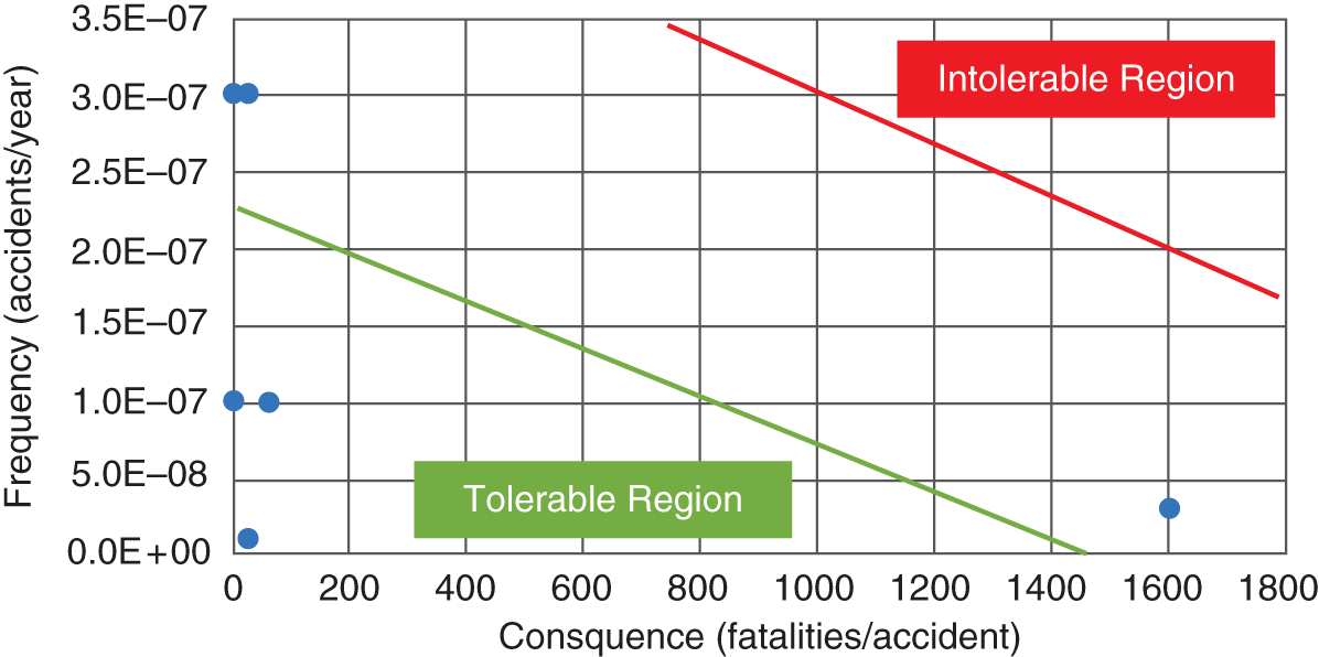
Figure 12.8 Overall societal risk consequence vs. frequency (zoomed).
To prioritize risks, first, the risks in the intolerable region must be addressed. Then, the risks in the ALARA region should be evaluated further to decide if they can be deemed tolerable for reasons such as impractical mitigation methods or cost of correction exceeding improvements gained. ALARA risks deemed intolerable should be corrected next. Lastly, risks in the tolerable region do not need any modifications unless the consequence or frequency increases. Risks in the tolerable region only need to be monitored to ensure they do not worsen and cross into the ALARA or intolerable region. Table 12.13 depicts risks, their region, and a description of the risk, consequence, and frequency value.
Table 12.13 A table for overall societal risk.
| Region | Risk | Type | Risk description | Consequence (fatalities/accident) | Frequency (accidents/year) |
|---|---|---|---|---|---|
| Intolerable | Forge | Fixed | Carbon monoxide, CO, is the main reducing agent in blast furnace gas | 8000 | 3.0E–07 |
| Intolerable | Gas transportation | Transportation | Gas (petrol) is transported from the gas distribution center to gas stations across the city | 32 | 3.0E–06 |
| ALARA | Pest control service | Fixed | Phosgene is a main ingredient in pesticides | 28.8 | 3.0E–07 |
| ALARA | Composite wood manufacturer | Fixed | Formaldehyde is used in the manufacture of composite wood products | 3 | 3.0E–07 |
| ALARA | Gas distribution center | Fixed | Gas (petrol) is stored to be distributed to gas stations around the city | 1600 | 3.0E–08 |
| ALARA | Ice rink | Fixed | Ammonia is used in the refrigeration system | 9.6 | 3.0E–07 |
| Tolerable | Bus garage | Fixed | Petrol is used and stored to fuel buses | 36 | 1.0E–08 |
| Tolerable | Competition pool | Fixed | Chlorine is used and stored to keep the pool water clean and healthy | 5.4 | 1.0E–07 |
| Tolerable | Sugar refinery | Fixed | Sulfur dioxide is used as a decolorizer in sugar | 2.4 | 1.0E–07 |
| Tolerable | Chlorine transportation | Transportation | Chlorine is transported from the port and delivered to pools across | 64 | 1.0E–07 |
12.2.6 Recommendations
The following recommendations are based on the results of the assessment and risk prioritization in Section 12.2.5:
12.2.6.1 Forge
The forge has a high risk because it has a very high consequence. Therefore, the focus should be on lowering the consequence of an accident. With the current capacity and production of blast furnace gas (BFG), even if BFG is disposed of daily, the amount of carbon monoxide produced would still be above 10,000 tons, meaning an effect category of HIII. To reduce the amount of BFG produced, the forge should slow down production, thus reducing the BFG produced and changing the effective category, decreasing the maximum effective distance and area. In addition, the forge could also find a way to reuse the BFG, minimizing the amount of BFG created. If the amount of carbon monoxide and BFG produced can be decreased from over 16,000 tons to 10,000 tons or less, the effect category would be GIII rather than HIII, thus reducing the maximum effective distance from 10,000 m to 3,000 m. Also, the affected area will decrease from 1,000 ha to 300 ha. This could bring the consequence from 8,000 fatalities per accident to 2,400 fatalities per accident. Alternatively, if neither of those can be done, or results are insufficient, the forge should move and open a new location in a large area with a low population. Ideally, this area should be at least 10,000 m away from the nearest town since that is the current maximum effect distance. If these changes could be accomplished, this risk would then be in the ALARA region.
12.2.6.2 Gas Transportation
This transportation route has a high frequency of accidents, so the focus should be on lowering this. To lower the frequency of accidents, the route the truck drives could be changed to divert the truck to less busy roads with little to no traffic, increasing the safety of areas with large populations in the city. This change will increase the probability correction parameter for wind direction toward populated areas (np) and the safety conditions of transport systems (nc). Currently, np has a value of 0 because people live in most of the effect area. However, a better path can be found where the part of the area where people are living only covers 50% or less of the effect area, np can increase from a value of 0 to +0.5. In addition, diverting the route to a less populated area could increase nc from a value of 0 to +1. These increases in value would bring Nt,s from 5.5 to 7, decreasing P from 3E–06 to 1E–7. If these changes could be achieved, this risk would be in the tolerable region.
12.2.6.3 Pest Control Service
The risk related to the pest control service is in the ALARA region for risk because of its frequency. If this risk is determined to be tolerable, nothing will be done. However, suppose this risk is determined to be an intolerable risk. In that case, the accident frequency can be decreased by having the company implement more safety measures in their facility, thus increasing their probability number correction parameter for organizational safety (no). Currently, the pest control service only practices the average industry safety standards. If the company can increase its safety regulations to above the industry standard, it can increase their no from 0 to +0.5. This increase would bring their Nt,s from 6.5 to 7, decreasing their P value from 3E–7 to 1E–7. If this is not possible, the company could move its location to farther outside the city, diminishing the population in the affected area and increasing the probability number correction parameter for wind direction toward populated areas in the affect zone, np. Currently, np has a value of 0 because most of the affected area has a population living there. If the company moves to a place where 50% or less of the population lives in the affected area, the np value could increase from 0 to +0.5, +1, or +1.5. These values would increase Nt,s from 6.5 to 7, 7.5, or 8, respectively, thus decreasing P from 3E–7 to 1E–7, 3E–8, or 1E–8, respectively. This risk would be in the tolerable region if these changes could be accomplished.
12.2.6.4 Composite Wood Manufacturer
The risk caused by the composite wood manufacturer is in the ALARA region for risk because of its higher frequency. If this risk is determined to be tolerable, nothing will be done. However, if this risk is considered intolerable, a few changes can be made. Like the pest control service, the composite wood manufacturer could implement higher safety measures in the facility, bringing the value of no from 0 to +0.5. Again, this increase would increase their Nt,s from 6.5 to 7, decreasing their P value from 3E–7 to 1E–7. This risk would be in the tolerable region if these changes could be accomplished.
12.2.6.5 Gas Distribution Center
The risk caused by the gas distribution center is in the ALARA region because of its high consequence. If this risk is determined to be tolerable, nothing will be done. However, if this risk is determined to be an intolerable risk, a few changes can be made. To decrease the risk, the center could be forced to lower the amount of petrol they can have at a time, lowering the effective category, which also reduces the maximum affected distance and area. Currently, the amount of petrol stored is 4,871 tons, leading to an effect category of EII. If the amount of petrol stored can be decreased to 200–1000 tons, the new effect category would be DII. With this category, the maximum effect distance would drop from 500 m to 200 m, and the effect area would decrease from 40 ha to 6 ha. This change would bring the consequence from 1,600 fatalities per accident to 240 deaths per accident. This risk would be in the tolerable region if these changes could be accomplished.
12.3 Vulnerability Assessment
The Vulnerability Assessment (VA) aims to assess the vulnerabilities of physical assets throughout the city, develop countermeasures, estimate costs, and develop a better plan to protect the city and its citizens against future attacks. The Guide to Highway Vulnerability Assessment for Critical Asset Identification and Protection (Science Applications International Corporation 2002) is used to perform the VA for the selected area of Portland. This approach consists of six main steps:
- identification of critical routes and assets
- assessment of vulnerabilities
- assessment of consequences
- identification of countermeasures
- estimation of countermeasure costs
- security operational planning development
12.3.1 Step 1: Identify Critical Routes and Assets
The comprehensive plan vision for Portland is as follows (City of Portland 2022):
Portland is a prosperous, healthy, equitable and resilient city where everyone has access to opportunity and is engaged in shaping decisions that affect their lives
Taking this mission statement, five critical routes are identified. Two different routes from the trade port to a pool are identified, as well as three routes from the gas distribution center to a popular gas station. Figure 12.9 depicts the routes involved. These routes involve the transportation of hazardous goods.

Figure 12.9 Identification of critical routes.
These five routes all cross over one intersection, so this intersection is evaluated in more detail. Four critical assets relating to the mission statement surround this intersection, including a bank, school, bus station, and hospital, thus making this intersection a critical intersection. Therefore, there are now five essential assets of this area, which will be evaluated in further detail throughout this assessment. Figure 12.10 shows the location of each critical asset.

Figure 12.10 Identification of critical assets.
Once identified, each critical asset is categorized as infrastructure, facilities, equipment, or personnel, as suggested in Table 12.14. The critical infrastructure (CI) – bus station, school, hospital, and bank – will be the main focus throughout this assessment. Still, the equipment and personnel of those facilities will be used for more detailed analysis when necessary.
Table 12.14 Categorization of critical assets of the city.
| Critical city assets | |||
|---|---|---|---|
| infrastructure | Facilities | Equipment | Personnel |
| Critical intersection | Bus station | Public buses | Bus drivers |
| School | School buses | Teachers | |
| Hospital | Ambulances | Bank tellers | |
| Bank | Doctors/Nurses | ||
Once critical routes and assets are identified, critical asset scoring must be completed. This is done through established critical asset factors and a value assigned to each factor. The value assigned to each factor will be ranked on a scale of 1 to 5, 1 being of very little importance and 5 being extremely important. Using Science Applications International Corporation’s (2002) guide, Table 12.15 is developed to show each critical asset factor, its value, and a description of the factor. Next, each of the five main critical assets is scored against the factors established in Table 12.15, as suggested in Table 12.16, indicating the most critical assets. And in this case, the hospital is the most critical, followed by the school and the critical intersection. The bus station and the bank are the least critical. This concludes Step 1 of the VA.
Table 12.15 Critical assets factors.
| Critical asset factor | Value | Description |
|---|---|---|
| Deter/defend factors | ||
| A) Ability to provide protection | 1 | Does the asset lack a system of measures? |
|
B) Relative vulnerability | 2 |
Is the asset relatively vulnerable to an attack? |
| Loss and damage Consequences | ||
| C) Casualty risk | 5 | Is there a possibility of serious injury or loss of life resulting from an attack on the asset? |
| Consequence to public services | ||
| D) Emergency response function | 5 | Does the asset serve an emergency response function and will the action or activity of the emergency response be affected? |
| E) Transportation | 1 | Will an attack on the asset affect the ability for transportation around the city? |
| Consequence to general public | ||
| F) Economic impact | 4 | Will damage to this asset have an effect on the means of living, resources or wealth of the city and those in |
| G) Health and care | 4 | Does this asset serve to assist with the health and care for citizens of the city? |
| H) Education | 1 | Will an attack on this asset affect access to education? |
Table 12.16 Scoring critical assets.
| Critical asset factor | Value | Description |
|---|---|---|
| Deter/defend factors | ||
| A) Ability to provide protection | 1 | Does the asset lack a system of measures? |
| B) Relative vulnerability | 2 | Is the asset relatively vulnerable to an attack? |
| Loss and damage consequences | ||
| C) Casualty risk | 5 | Is there a possibility of serious injury or loss of life resulting from an attack on the asset? |
| Consequence to public services | ||
| D) Emergency response function | 5 | Does the asset serve an emergency response function and will the action or activity of the emergency response be affected? |
| E) Transportation | 1 | Will an attack on the asset affect the ability for transportation around the city? |
| Consequence to general public | ||
| F) Economic impact | 4 | Will damage to this asset have an effect on the means of living, resources, or wealth of the city and those in nearby areas |
| G) Health and care | 4 | Does this asset serve to assist with the health and care for citizens of the city? |
| H) Education | 1 | Will an attack on this asset affect access to education? |
12.3.2 Step 2: Assess Vulnerabilities
Step 2 identifies and evaluates critical assets regarding their weaknesses and other vulnerabilities. Each critical asset is scored against multiple vulnerability factors. These vulnerability factors included visibility and attendance, access to the asset, and site-specific hazards. Each of these three factors is broken into two sub-elements. Factors and their sub-elements are as follows:
- Visibility and attendance
- – Level of recognition (A)
- – Attendance/users (B)
- Access to the asset
- – Access proximity (C)
- – Security level (D)
- Site-specific hazards
- – Receptor impacts (E)
- – Volume (F)
Each asset’s vulnerability is scored on a scale of 1 to 5 based on a table in Science Applications International Corporation’s (2002) research, which described each level of the scale for each vulnerability factor sub-element. Once each critical asset’s vulnerability is scored against the six sub-elements, the total vulnerability score, y, is calculated using Equation (12.5).
Table 12.17 depicts the results from the vulnerability factor scoring. These results show that the bus station is the most vulnerable asset, followed by the hospital, intersection, school, and bank, consecutively. This concludes Step 2.
Table 12.17 Vulnerability factor scoring.
| Critical asset | Vulnerability factor |
Total score(y) | |||||||
|---|---|---|---|---|---|---|---|---|---|
| (A * B) | + | (C * D) | + | (E * F) | |||||
| 1–5 | 1–5 | 1–5 | 1–5 | 1–5 | 1–5 | ||||
| School | 4 | 3 | 5 | 3 | 2 | 3 | 33 | ||
| Bus station | 2 | 2 | 5 | 5 | 4 | 4 | 45 | ||
| Hospital | 4 | 5 | 5 | 2 | 4 | 3 | 42 | ||
| Bank | 5 | 3 | 5 | 1 | 2 | 3 | 26 | ||
| Critical intersection | 2 | 2 | 4 | 5 | 4 | 4 | 40 | ||
12.3.3 Step 3: Assess Consequences
Step 3 is to identify assets with the most significant risk based on the asset’s criticality and vulnerability. The critical asset scoring completed in Step 1 and the vulnerability factor scoring in Step 2 are used to determine the criticality and vulnerability assets. Equations (12.6) and (12.7) are used to plot the criticality vs. vulnerability of each asset.
where x is the critical asset score for each critical asset, Cmax is the maximum critically score (which in this case is 23), and y is the vulnerability score for each critical asset. By using these equations, X and Y for each asset could be calculated. These calculations are shown in Table 12.18.
Table 12.18 Criticality and vulnerability of assets.
| Critical asset | x | X = (x/Cmax)*100 | Y | Y = (y/75)*100 | Quadrant |
|---|---|---|---|---|---|
| School | 13 | 57 | 33 | 44 | II |
| Bus station | 12 | 52 | 45 | 60 | I |
| Hospital | 21 | 91 | 42 | 56 | I |
| Bank | 12 | 52 | 26 | 35 | II |
| Critical intersection | 13 | 57 | 40 | 53 | I |
A criticality and vulnerability matrix with four quadrants is then developed. Critical assets located in Quadrant I have high criticality and high vulnerability. Assets in Quadrant II have low criticality and high vulnerability. Assets in Quadrant III have low criticality and low vulnerability. Assets in Quadrant IV have high criticality and low vulnerability. Figure 12.11 depicts the criticality and vulnerability matrix. This concludes Step 3.

Figure 12.11 Criticality vs. vulnerability matrix.
12.3.4 Step 4: Identify Countermeasures
Step 4 is to identify typical countermeasures to protect critical assets against an attack. Table 12.19 depicts a list of proposed countermeasures, the corresponding critical asset category, and the countermeasure function adapted from Science Applications International Corporation (2002).
Table 12.19 Countermeasures for critical assets.
| Countermeasure | Critical asset category | Countermeasure function | |||||
|---|---|---|---|---|---|---|---|
| Infrastructure | Facilities | Equipment | Personnel | Detect | Deter | Defend | |
| Ensure there are full-time security guards on the property guarding all main entrances | X | X | X | ||||
| Keep all non-main access points locked and install motion-sensored security cameras around those access points | X | X | X | ||||
| Have a front desk by the main entrance that all guests/visitors have to sign in at | X | X | X | ||||
| Implement bag checks and install metal detectors at main entrances | X | X | X | X | |||
| Install more light fixtures | X | X | X | X | X | X | |
| Install barriers around entrances / seating areas to prevent easy and quick access for vehicles | X | X | X | X | X | ||
| Install bullet-proof windows on counters/desks/vehicles that others may have easy access to | X | X | X | X | X | ||
| Add motion sensors to fences | X | X | X | X | |||
| Implement frequent safety trainings for employees and customers in case of an emergency | X | X | X | ||||
| Limit access with building badges for employees and visitors | X | X | X | X | |||
| Install full-time security cameras with video capability at critical assets | X | X | X | X | X | X | |
| Implement full-time surveillance at critical assets | X | X | X | X | X | X | |
12.3.5 Step 5: Estimate Countermeasure Costs
Step 5 estimates the capital, operating, and maintenance costs of the countermeasures proposed in Step 4. All countermeasures are broken down into “packages” based on the critical asset category that the countermeasure would assist. These “packages” are based on the “Critical asset category” column from Table 12.19. If a countermeasure is applied to a critical asset category, it is added to that critical asset category’s package. Each type of cost is determined to be high (H), medium (M), or low (L) based on values from Science Applications International Corporation (2002). Costs are determined based on estimates and data from Science Applications International Corporation (2002). The countermeasure function column is the same as the information found in Table 12.19. Table 12.20 shows the countermeasure cost estimates for infrastructure. Table 12.21 shows the countermeasure cost estimates for facilities. Table 12.22 shows the countermeasure cost estimates for equipment. Table 12.23 shows the countermeasure cost estimates for personnel.
Table 12.20 Infrastructure countermeasure cost estimates.
| Countermeasure | Critical asset category | Countermeasure function | |||||
|---|---|---|---|---|---|---|---|
| Infrastructure | Facilities | Equipment | Personnel | Detect | Deter | Defend | |
| Ensure there are full-time security guards on the property guarding all main entrances | X | X | X | ||||
| Keep all non-main access points locked and install motion-sensored security cameras around those access points | X | X | X | ||||
| Have a front desk by the main entrance that all guests/visitors have to sign in at | X | X | X | ||||
| Implement bag checks and install metal detectors at main entrances | X | X | X | X | |||
| Install more light fixtures | X | X | X | X | X | X | |
| Install barriers around entrances / seating areas to prevent easy and quick access for vehicles | X | X | X | X | X | ||
| Install bullet-proof windows on counters/desks/vehicles that others may have easy access to | X | X | X | X | X | ||
| Add motion sensors to fences | X | X | X | X | |||
| Implement frequent safety trainings for employees and customers in case of an emergency | X | X | X | ||||
| Limit access with building badges for employees and visitors | X | X | X | X | |||
| Install full-time security cameras with video capability at critical assets | X | X | X | X | X | X | |
| Implement full-time surveillance at critical assets | X | X | X | X | X | X | |
Table 12.21 Facilities countermeasure cost estimates.
| Critical asset group | Countermeasure |
Countermeasure function | Estimated relative cost (H/M/L) | ||||
|---|---|---|---|---|---|---|---|
| Detect | Deter | Defend | Capital | operating | Maintenance | ||
|
Equipment: Public buses School buses Ambulances | Install more light fixtures | X | x | L | L | L | |
| Install barriers around entrances/seating areas to prevent easy and quick access for vehicles | x | X | L | L | L | ||
| Install bullet-proof windows on counters/desks/vehicles that others may have easy access to | x | X | M | L | L | ||
| Add motion sensors to fences | X | x | L | L | L | ||
| Implement frequent safety trainings for employees and customers in case of an emergency | X | L | L | L | |||
| Limit access with building badges for employees and visitors | X | L | L | L | |||
| Install full-time security cameras with video capability at critical assets | X | X | H | M | L | ||
| Implement full-time surveillance at critical assets | X | X | H | H | H | ||
Table 12.22 Equipment countermeasure cost estimates.
| Critical asset group | Countermeasure | Countermeasure function | Estimated relative cost (H/M/L) | ||||
|---|---|---|---|---|---|---|---|
| Detect | Deter | Defend | Capital | Operating | Maintenance | ||
|
Facilities: Bus station School Hospital Bank | Ensure there are full-time security guards on the property guarding all main entrances | X | X | M | M | L | |
| Keep all non-main access points locked and install motion-sensored security cameras around those access points | X | X | H | M | L | ||
| Have a front desk by the main entrance that all guests/visitors have to sign in | X | L | L | L | |||
| Implement bag checks and install metal detectors at main entrances | X | X | L | M | L | ||
| Install more light fixtures | X | X | L | L | L | ||
| Install barriers around entrances/seating areas to prevent easy and quick access for vehicles | X | X | L | L | L | ||
| Install bullet-proof windows on counters/desks/vehicles that others may have easy access to | X | X | M | L | L | ||
| Add motion sensors to fences | X | X | L | L | L | ||
| Limit access with building badges for employees and visitors | X | L | L | L | |||
| Install full-time security cameras with video capability at critical assets | X | X | H | M | L | ||
|
Implement full-time surveillance at critical assets | X | X | H | H | H | ||
Table 12.23 Personnel countermeasure cost estimates.
| Critical asset group | Countermeasure | Countermeasure function | Estimated relative cost (H/M/L) | ||||
|---|---|---|---|---|---|---|---|
| Detect | Deter | Defend | Capital | Operating | Maintenance | ||
|
Personnel: Bus drivers Teachers Bank tellers Doctors/nurses | Have a front desk by the main entrance that all guests/visitors have to sign in at | X | L | L | L | ||
| Implement bag checks and install metal detectors at main entrances | X | X | L | M | L | ||
| Install more light fixtures | X | X | L | L | L | ||
| Install barriers around entrances/seating areas to prevent easy and quick access for vehicles | X | X | L | L | L | ||
| Install bullet-proof windows on counters/desks/vehicles that others may have easy access to | X | X | M | L | L | ||
| Implement frequent safety trainings for employees and customers in case of an emergency | X | L | L | L | |||
| Limit access with building badges for employees and visitors | X | L | L | L | |||
| Install full-time security cameras with video capability at critical assets | X | X | H | M | L | ||
| Implement full-time surveillance at critical assets | X | X | H | H | H | ||
12.3.6 Step 6: Security Operational Planning Development
An operational security plan is meant to prevent potential risks and consequences. The plan includes developing countermeasures, such as training and exercises, as well as other security measures. The scope for an operational security plan for Portland would be as follows:
To identify and prevent risks to protect personnel, deter criminal and/or terrorist activities and eliminate unauthorized access to critical assets.
Cloutier (2021) suggests a five-step process for operational security plans:
- identify critical information
- analyze threats
- analyze vulnerabilities
- assess the risk
- determine countermeasures
These five steps are very similar to the steps in the VA. During these steps, critical information is identified by determining the critical assets of the area (VA Step 1). Threats are analyzed after establishing and assigning values to the critical asset factors (VA Step 1). Vulnerability is analyzed during the VA Step 2. The risk is assessed during the VA Step 3, where the consequence of risk on each critical asset is assessed. And finally, during the VA Steps 4–5, countermeasures are identified as well as the estimated cost for each countermeasure.
Now that those activities have been completed during this VA for Portland, the next step of the operational security plan is to implement the countermeasures. Once implemented, the success of the countermeasure would be evaluated to determine if the results are satisfactory or not. If the results are not satisfactory, these five steps would be repeated until the results are satisfactory.
12.4 IRRA of Air, Water, and Ground Pollution
The IRRA aims to analyze continuous emission sources and evaluate their impact on the city’s citizens’ health. Dangerous goods and hazardous materials are some of the most significant pollution causes in a city like Portland. Unfortunately, the largest producers of those same dangerous goods and hazardous materials are the large manufacturers and consumer products within that city. The transportation of these dangerous goods and hazardous materials further adds to the pollution within the city. The manufacturing and transportation of these materials create emissions that can cause adverse amounts of pollution in the air, water, and soil in and around the city. The Guidelines for Integrated Risk Assessment and Management in Large Industrial Areas (International Atomic Energy Agency 1998) are used to analyze continuous emissions in the city. These guidelines outline seven steps:
- identify sources of continuous emission
- characterize the emission source inventory
- select a pathway for analysis organized according to the receiving media: air, water, soil
- use models calculate dispersion values
- (if necessary) evaluate the concentration of pollutants as a time-distance function by using atmospheric dispersion models
- use air quality, water quality, and soil quality standards or dose–response relationships to estimate the risk to the population; evaluate the health impacts
- use analytical methods, critical load concepts or expert judgment for environmental impact assessment
An in-depth analysis of emissions for Portland is outside the scope of the present research. Only three sources of continuous emissions in Portland are selected, as depicted in Table 12.24. In Sections 12.4.1–12.4.5, individual pollution maps for each source are unavailable, so multiple maps will be used to describe the emissions.
Table 12.24 Suggested continuous sources of emissions.
| Source | Pollutant | Emission coefficient | Description |
|---|---|---|---|
| Gas distribution center | NO2 | 136.98 | Underground gas storage – 5000 acres 6 × 10¹⁰ scf/yr capacity |
| Landfill | NO2 | 0.42 | Commercial waste repository – construction and operations emissions |
| Power plant | NO2 | 850.00 | Coal-fired power plant, western coals – conv. steam plant; emissions controls |
12.4.1 Airborne (Air Pollution)
Figure 12.12 is taken from AQICN (https://aqicn.org/city/usa/oregon/portland) and shows Portland’s real-time air quality index as of Saturday, April 16, 2022 at 3 p.m. This map shows places where air quality is measured. As shown in the map, all the measurements in Portland are green, meaning the air quality is considered “good” and minimal pollutants are detected in the air.

Figure 12.12 Real-time air quality in Portland.
AQICN also lists changes in air quality over the last forty-eight hours. Figure 12.13 breaks down pollution by different air pollutants and lists the minimum and maximum values for each. The overall air quality in Portland is an 18, which is considered “good.” The lower the number, the better the air quality because fewer pollutants are detected. This figure also shows that the pollution consists of mainly fine particle matter (PM2.5) and nitrogen dioxide (NO2). NO2 is found in pollution from all three sources of continuous emissions listed previously, which all contribute to the total emission count for the city.

Figure 12.13 Air quality data for the past forty-eight hours.
AQICN also displays historical data related to air pollution. For example, Figure 12.14 shows the daily data for NO2 from 2020 to April 16, 2022. This figure shows that over the last few years, a low amount of NO2 has been detected in emissions. Therefore, despite many continuous emission sources throughout the city, they do not produce an overwhelming or dangerous amount of NO2.

Figure 12.14 Annual air pollution data.
12.4.2 Waterborne (Water Pollution)
EnviroAtlas (https://www.epa.gov/enviroatlas) shows water pollution throughout the Portland area. Figure 12.15 shows all impaired waterways in red, while Figure 12.16 shows the waterways that are assessed in blue. These waterways are assessed and determined to be impaired as they are degraded and do not meet the standards for many designated beneficial uses, such as aquatic life and drinking water.

Figure 12.15 Impaired waterways.

Figure 12.16 Assessed waterways.
Nitrate violations in surface water systems are also a concern. Again, higher values indicate a higher probability of a violation. This violation means more nitrate, such as NO2, is in the surface water system than is allowed or safe. Overall, Portland has a better-than-average probability of a violation of nitrate in a surface water system, according to the scale in Figure 12.17. However, the northern outskirts of Portland have a higher probability, so the previously listed sources of continuous emissions, or similar sources, are likely found in those areas. Areas south of Portland have a lower probability of a violation, so there are likely not as many continuous emissions sources. Overall, there is little pollution in the surface water system in the center and other main areas of Portland, unlike the outskirts.

Figure 12.17 Surface water violation index.
Figure 12.18 shows the nitrate violation in groundwater systems. A water quality index map from 2020 is shown in Figure 12.19. This map displays the water quality in certain areas in and around Portland and whether that measurement is better or worse or if there is no change from the previous year.

Figure 12.18 Groundwater violation index.

Figure 12.19 Water quality index map.
12.4.3 Soil (Ground Pollution)
EnviroAtlas can also show the movement of nitrogen attached to the soil particles eroding from the surface of agricultural fields, as depicted in Figure 12.20. Green areas have smaller amounts of nitrogen than blue or purple areas. High levels of nitrogen movement mean there is likely a high level of breakdowns of nitrates, meaning there could be a lot of pollution, such as NO2, in the soil. Areas shaded in blue or purple have higher nitrogen levels, indicating a higher probability of pollution in the soil. NO2 is found in the three sources of continuous emissions listed previously, meaning those sources or similar locations are likely located in the outskirts of Portland. Therefore, the soil on the edges of Portland has more pollution than the soil in the city’s center. Again, this makes sense because the areas on the outer edges, specifically the northern area of Portland, are more commercial and industrial than the center of Portland, which is more residential.

Figure 12.20 Surface soil pollution.
12.4.4 Risks and Associated Consequences
The more pollution in the environment (i.e. air, water, ground), the more at-risk the city’s citizens are. These risks can lead to consequences, including mortality and morbidity. Air pollution is the most significant risk to the health of the citizens in the city. Citizens who spend the most time in risk areas are more likely to develop health problems in the future. Figure 12.21 shows the cancer risk per million due to cumulative air toxics. Figure 12.22 shows respiratory risk due to cumulative air toxics. Interestingly, these numbers suggest that all people in Portland have the same risk category (i.e. they all have the same risk of developing cancer and respiratory issues due to air toxics, including pollution). Figure 12.23 depicts the risk of developing a non-cancer neurological risk due to cumulative air toxics, including pollution. Figure 12.24 shows the risk of cancer due to formaldehyde air toxics. Figure 12.25 shows the respiratory risk due to formaldehyde air toxics.

Figure 12.21 Cancer risk due to cumulative air toxics.

Figure 12.22 Respiratory risk due to cumulative air toxics.

Figure 12.23 Non-cancer neurological risk due to cumulative air toxics.

Figure 12.24 Cancer risks due to formaldehyde air toxics.

Figure 12.25 Respiratory risk due to formaldehyde air toxics.
Although the data in both figures use different data and units to create their scales, the same color codes represent similar risk levels. The majority of Portland is all the same color, meaning the same risk. This makes sense because all buildings, including residential homes, businesses, apartment buildings, etc. have floors and furniture made from composite wood. Assuming these items are dispersed equally throughout the city among all buildings, the entire city has the same risk. Therefore, all citizens in Portland have roughly the same chance of developing the two issues due to formaldehyde.
12.4.5 EMP Assessment
EMP Assessment (EMPA) assesses EMP in an area at varying heights. EMP is a pulse of high-intensity electromagnetic radiation generated especially by a nuclear blast high above the earth’s surface and held to disrupt electronic and electrical systems (Zhang et al. 2022). EMP has the potential to affect extensive areas. If an area is affected, CIs will be severely impacted (National Coordinating Center for Communications 2019). EMP devices, including weapons and missiles, can explode in the air and release an electromagnetic wave, disrupting the electrical grid and causing damage to electronics such as computers, cell phones, radios, etc. (Cybersecurity and Infrastructure Security Agency 2022). Figure 12.26 visually represents how a high-altitude EMP detonation affects an area when it explodes (Security Team 2022).

Figure 12.26 A high-altitude EMP detonation.
The area that an EMP explosion covers depends on the height of the explosion. The EMP radius can be determined as long as the height of the burst (HOB) is known. The HOB and EMP radius are related using Equation (12.8) (EMPEngineering.com 2022; National Coordinating Center for Communications 2019).
The following analysis calculates how large the EMP radius would be if the HOB is at 25 km, 100 km, and 400 km above the center of Portland, and discusses which areas would be affected at each HOB. Since Portland is on the west coast, less land will be directly affected than if the blast occurred in a more central state, so the blast will also cover parts of the Pacific Ocean. If there are ships in the affected area, their electronics, such as radios, can be damaged too. Using Equation (12.8), a HOB of 25 km, the EMP radius is:
At the height of 25 km, the entire state of Oregon and Ishington area would be affected, including surrounding states as well as parts of Canada, as depicted by Figure 12.27.

Figure 12.27 EMP detonation at a HOB of 25 km.
At the height of 40 km, the entire state of Oregon and Ishington would be affected, including parts of Canada, Idaho, California, and Nevada, as suggested by Figure 12.28. At the height of 400 km, roughly 50% of the United States and Canada and Mexico would be affected, as suggested in Figure 12.29.

Figure 12.28 EMP detonation at a HOB of 100 km.

Figure 12.29 EMP detonation at a HOB of 400 km.
Figure 12.30 depicts EMP radius for the HOBs at 25 km, 40 km, 100 km, and 400 km, allowing for a better comparison of how the height affects EMP radius.
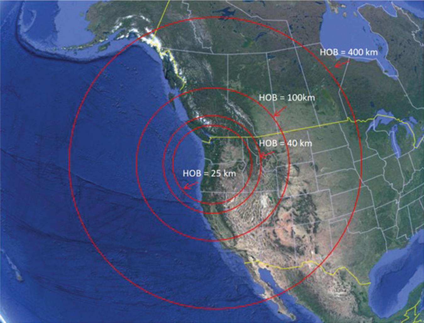
Figure 12.30 EMP radius for varying height of bursts.
From all these figures, it is easy to see how an EMP blast in Portland could affect many areas across the continent. EMP blasts can be detrimental to a country because an extremely large area can be affected by just one blast. More specifically, if the blast is released above a location more in the center of the country, such as Omaha, NE, the blast could have the potential to affect practically all of the contiguous United States, as well as parts of Canada and Mexico, if the blast occurred at 400 km, as suggested by Figure 12.31.

Figure 12.31 A HOB of 400 km above Omaha (approximately).
Preventing an EMP attack is impossible, and reducing its effects is challenging (Electromagnetic Pulse Commission 2008). However, the Department of Homeland Security mitigates risks (Cybersecurity and Infrastructure Security Agency 2022).
12.5 Comprehensive Implementation Plan for ReIDMP
Again, “resilience” has no single widely accepted definition (Gheorghe and Katina 2014; Katina and Gheorghe 2023; Vasuthanasub 2019). The goal of the design process is to develop a resilient system. This is important early in the design process, where informed decisions are made to ensure the developed system is resilient. Considerations of resilience must occur early in the design process because that is when there is the most freedom to explore design alternatives. A resilient developed system is capable of preventing/avoiding, mitigating, and recovering from failures, unlike reliability engineering, which only focuses on avoiding risks at all costs (Hulse 2019). The ReIDMP model is intended to develop a process that ends with a product/system that is created with resiliency in mind, including a city. Figure 12.32 depicts a simplified version of the ReIDMP presented in Chapter 7. The final product/system should be a resilient system capable of preventing, mitigating, and recovering from failures. Again, the ReIDMP model is grounded in RRA, VA, and IRRA and enables informed decisions for developing resilient systems.

Figure 12.32 A revised ReIDMP model.
The framework initially starts with city officials, and the same officials decide when the RRA, VA, and IRRA should be conducted. The same officials contact contractors and subject matter experts to conduct the three assessments – RRA, VA, and IIRA. Once RRA, VA, and IIRA are completed, the results are presented to the city officials, regional officials, other governance board members, and stakeholders, who will discuss topics of grave concern. Together, they will prioritize and categorize these concerns and determine whether they would need risk prevention, mitigation, and/or recovery after the risk occurs. A possible course of action is developed and implemented to address risks and vulnerabilities.
In this case, we can see that city officials can apply the ReIDMP to develop a resilient city with relative ease. Moreover, incorporating resilience into a solution or plan can lead to a more economical solution, especially for those involved in improving city safety through prevention, mitigation, and recovery (Hulse 2019).
12.6 Concluding Remarks
In this chapter, multiple assessments are performed on the City of Portland, including the RRA, VA, and IRRA. These assessments used the methodologies from the Manual for the Classification of Prioritization of Risks Due to Major Accidents in Process and Related Industries (International Atomic Energy Agency 1996), Guide to Highway Vulnerability Assessment for Critical Asset Identification and Protection (Science Applications International Corporation 2002), and Guidelines for Integrated Risk Assessment and Management in Large Industrial Areas (International Atomic Energy Agency 1998). These assessments help determine significant fixed risks and risks related to the transportation of hazardous goods, the vulnerability of critical assets, and the effect of different emissions throughout the city. With these assessments, risks are prioritized to determine which activities cause the most significant threats to the health and safety of citizens and visitors in the city. Prioritizing risk activities and vulnerabilities allows city officials to determine risks and implement viable solutions to decrease the consequence and/or frequency of risks – making a city safer and healthier.
An EPA is also performed to analyze the effects of an EMP blast at varying heights above Portland. Although reducing the effects of EMP blasts is difficult, it is important to understand how they work and the damage they can cause. We suggest that using these models can allow city officials to make resilient-informed decisions and take action to develop resilient cities.
12.7 Exercises
1 Discuss how RRA can enhance the decision-making process for Portland city leaders.
2 Discuss how VA can enhance the decision-making process for Portland city leaders.
3 Discuss how IRRA can enhance the decision-making process for Portland city leaders.
4 Discuss how EMPA can enhance the decision-making process for Portland city leaders.
5 Discuss how you would implement ReIDMP analysis results for the City of Portland.
References
- City of Portland. (2022). Portland’s Vision for Growth and Progress [ Portland.com]. https://www.portland.gov/bps/planning/comp-plan/vision-growth-and-progress.
- Cloutier, R. (2021, November 5). What is Operational Security? The Five-step OPSEC Process [Cybersecurity]. Security Studio. https://securitystudio.com/operational-security.
- Cybersecurity and Infrastructure Security Agency. (2022). Electromagnetic Pulse and Geomagnetic Disturbance. https://www.cisa.gov/emp-gmd.
- Electromagnetic Pulse Commission. (2008). Report of the Commission to Assess the Threat to the United States from Electromagnetic Pulse (EMP) Attack: Critical National Infrastructures. Prepper Press.
- EMPEngineering.com (2022). EMP/HEMP attacks. EMP Engineering. https://www.empengineering.com/emp-hemp-attacks
- Gheorghe, A.V. and Katina, P.F. (2014). Editorial: Resiliency and engineering systems – Research trends and challenges. International Journal of Critical Infrastructures 10 (3/4): 193–199. https://www.inderscience.com/info/dl.php?filename=2014/ijcis-4113.pdf.
- Hulse, D. (2019). A framework for resilience informed decision making in early design. Annual Conference of the PHM Society 11 (1): Article 1. https://doi.org/10.36001/phmconf.2019.v11i1.913.
- International Atomic Energy Agency. (1996). Manual for the Classification and Prioritization of Risks Due to Major Accidents in Process and Related Industries. International Atomic Energy Agency. http://www-pub.iaea.org/books/IAEABooks/5391/Manual-for-the-Classification-and-Prioritization-of-Risks-due-to-Major-Accidents-in-Process-and-Related-Industries.
- International Atomic Energy Agency. (1998). Guidelines for Integrated Risk Assessment and Management in Large Industrial Areas. International Atomic Energy Agency. http://www-pub.iaea.org/books/IAEABooks/5391/Manual-for-the-Classification-and-Prioritization-of-Risks-due-to-Major-Accidents-in-Process-and-Related-Industries.
- Katina, P.F. and Gheorghe, A.V. (2023). Blockchain-enabled Resilience: An Integrated Approach for Disaster Supply Chain and Logistics Management (1st ed.). CRC Press.
- National Coordinating Center for Communications. (2019). Electromagnetic Pulse (EMP) Protection and Resilience Guidelines for Critical Infrastructure and Equipment (Version 2.2). National Cybersecurity and Communications Integration Center. https://www.cisa.gov/sites/default/files/publications/19_0307_CISA_EMP-Protection-Resilience-Guidelines.pdf.
- O’Shea, C. (2021, June). How Montreal made ammonia safe for its rinks. HPAC Magazine. Annex Business Media. https://www.hpacmag.com/features/how-montreal-made-ammonia-safe-for-its-rinks.
- SafeRack. (2022). Chlorine handling design, loading, and installation. SafeRack. https://www.saferack.com/bulk-chemical/chlorine-loading-platforms.
- Science Applications International Corporation. (2002). Guide to Highway Vulnerability Assessment for Critical Asset Identification and Protection. Transportation Policy and Analysis Center.
- Security Team. (2022). EMP: A Real Threat. Aus Security Products. https://aussecurityproducts.com.au/blogs/posts/emp-a-real-threat.
- US Environmental Protection Agency. (2018). Ammonia Safety in New England Ice Rinks (overviews and factsheets EPA-901-F-18-001). US Environmental Protection Agency. https://www.epa.gov/indoor-air-quality-iaq/ammonia-safety-new-england-ice-rinks.
- Vasuthanasub, J. (2019). The resilient city: A platform for informed decision-making process. Dissertation, Old Dominion University. https://digitalcommons.odu.edu/emse_etds/151.
- Zhang, M., Li, H., and Liu, Q. (2022). Deep exploration on fault model of electromagnetic pulse attack. IEEE Transactions on Nanotechnology 21: 598–605. https://doi.org/10.1109/TNANO.2022.3214341.