
8
Analysis and Assessment of Risk and Vulnerability via Serious Gaming
8.1 Introduction
Risk and vulnerability assessments (VAs) are performed in many areas of engineering and technology. The goal of evaluating them is to be able to analyze potential impacts that can result in occurring of adverse events. In this research, the second phase of the Resilient-Informed Decision-Making Process (ReIDMP) is utilizing a product from SimCity as an applied visualization for technical analysis of risk and vulnerability. The specific techniques and procedures adopted in this investigation include assessments on potential accidents of hazmat processing at fixed installations and during transport activities, assessments on possible transportation routes regarding the critical assets, and assessments on health and environmental impacts from polluted byproducts generated by the industrial sector within the city and region. Altogether these analysis efforts improve the conceptual understanding of risks and vulnerabilities that are present in everyday society and how those exposures may affect the larger society as a whole. After the preceding stages, an informed decision-making process can be formalized to initiate and supervise a comprehensive plan promoting the city’s resilience.
8.2 Rapid Risk Assessment
To concurrently review rapid risk assessment (RRA) and modeled environment in SimCity application, the approach in Manual for the Classification and Prioritization of Risks due to Major Accidents in Process and Related Industries, (International Atomic Energy Agency 1996) is used. This document is also known as “IAEA-TECDOC-727 (Rev.1).” It represents the means to manage the risk of accidents regarding hazardous activities, such as fixed installations or transportation in the city or region of interest. The assessment method relies heavily on tables that have been developed based on historical information and input from subject matter experts (International Atomic Energy Agency 1996). By completing methodological procedures, the assessment results can give decision makers a holistic view of incentive information about the significant risks within the selected region.
8.2.1 Applications and Algorithm of RRA Methodology
According to the International Atomic Energy Agency (1996) IAEA-TECDOC-727 (Rev.1), the assessment process of each activity requires two calculating approaches to estimate the casualties per incident (consequence) and probabilities of occurrence (frequency). In the case of consequences, the estimation is defined by the number of fatalities. The number of fatalities is established using Equation 8.1 and the tables in IAEA-TECDOC-727 (Rev.1), as shown in Figure 8.1. Figure 8.2 is the continuation of the information in Figure 8.1.
 (8.1)
(8.1)
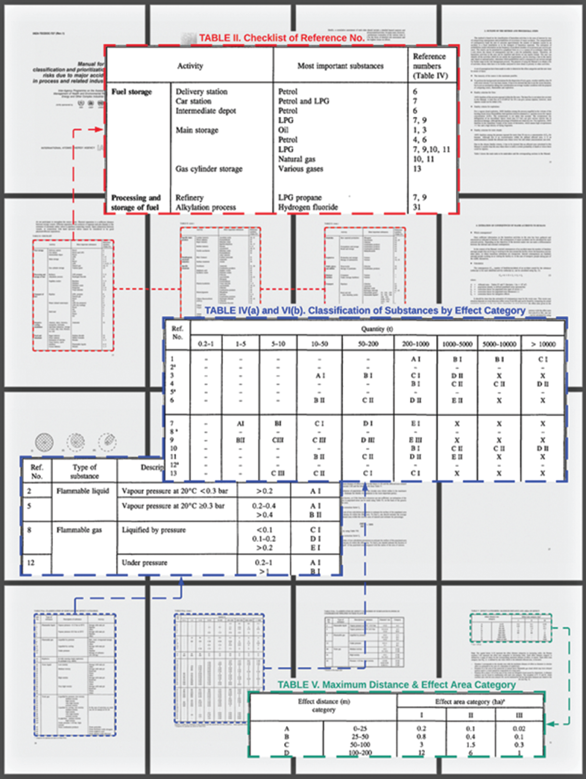
Figure 8.1 Example of information from tables used consequence estimation of major accidents.

Figure 8.2 Example of information from tables used consequence estimation of major accidents (continued).
where:
A = area affected by the incident (circle area)
D = population density within the affected area
CF1 = correction factor for the populated area (part of circle area)
CF2 = correction factor for the distance of effect category (radius of the circle)
CF3 = correction factor for mitigation at the selected facility
The following set of procedures is the sequential steps to obtain the constant of each variable in the equation of consequence estimation:
- Classify the activity using Table II and indicate reference numbers for Table IV(a) or IV(b).
- Determine the hazardous substance in each activity. Note that if multiple hazmats are presented in one location, both cannot be considered simultaneously. Alternatively, if hazardous materials are different in terms of effect area categories, such as flammable and toxic, they must be analyzed separately.
- Estimate the quantity of substances in each hazardous activity.
- Using Table IV, indicate the effect category code (related to the letters A–H and Roman numerals I–III).
- Indicate the maximum effective distance in meters, the affected area in hectares “A,” and the shape of the effect area category using Table V.
- Estimate the population density “D” within the affected area using Table VI.
- Estimate the distribution percentage of the existing population in the circular area in which radius is the maximum distance of effect. Then, obtain the correction factor “CF1” using Table VII.
- Estimate the distance area correction factor “CF2” based on the fraction distance (length or depth) in which populations exist within the effect radius of the circular area.
- Estimate the mitigation correction factor “CF3” using Table VIII.
- Calculate the external consequences “CA, S” using Equation 8.1.
The estimation of frequency is different from the estimation of consequence. The probability of occurrences is calculated based on the type of hazmat activities. The same generic equation and estimated procedures cannot assess both. For fixed installations or processing plants, the probability of a major accident is computed using Equation 8.2. The constant of each variable can be obtained by evaluating the information disclosed in the tables in IAEA-TECDOC-727 (Rev.1), as illustrated in Figure 8.3.
 (8.2)
(8.2)

Figure 8.3 Example of table information for estimating probability of major accidents for fixed installations of hazmat or dangerous goods.
where:
N*Fixed = average probability number for the facility and the substance
CP1 = correction parameter for the frequency of loading/unloading operations
CP2 = correction parameter for safety systems in cases of flammable substance
CP3 = correction parameter for the safety level at the facility
CP4 = correction parameter for wind direction toward a populated area
To proceed further in calculating the probability number of accidents at the fixed facilities with Equation 8.2, the guidance on how to determine the constant of each variable can be described as follows:
- Estimate the average probability number of an accident N*Fixed using Table IX.
- Estimate the probability number correction parameter for loading/unloading operations “CP1” using Table X.
- Using Table XI, estimate the probability number correction parameter for safety systems for flammable substances “CP2.”
- Estimate the probability number correction parameter for organizational and safety management aspects “CP3” using Table XII.
- Using Table XIII, estimate the probability number correction parameter for the wind direction toward populated areas “CP4.”
- Calculate the probability number “NFixed” using Equation 8.1.
- Convert the probability number “NFixed” into the frequency value “Pi,s” for the number of accidents per year using Table XIV.
In the cases of hazmat transportation, the probability number of a significant accident is calculated using Equation 8.3 and tables in IAEA-TECDOC-727 (Rev.1), as exhibited in Figure 8.3. Figure 8.4 is a continuation of Figure 8.3.

Figure 8.4 Example of table information for estimating probability of major accidents for transportations of hazmat or dangerous goods (continued).
 (8.3)
(8.3)
where:
N*Trans = average probability number for the transportation of the substance
CP5 = correction parameter for the safety conditions of substance transportation
CP6 = correction parameter for traffic density of the transportation route
CP7 = correction parameter for wind direction toward a populated area
The steps in defining numerical values in Equation 8.3 are similar to Equation 8.2. They are straightforward. The following are the instructions on how to assign the constant of each variable:
- Estimate the average probability number of transport category “N*Trans” using Table XV or XVI.
- Estimate the probability number correction parameter for the transport system “CP5” safety using Table XVII.
- Estimate the probability number correction parameter for traffic density “CP6” using Table XVIII.
- Estimate the probability number correction parameter for the wind direction toward populated areas “CP7” using Table XIX.
- Calculate the probability number “NTransport” using Equation 8.3.
- Using Table XX, convert the probability number “NTransport” into the frequency value “Pi,s” for the number of accidents per year.
Once the consequence value and frequency number of all potential accidents are calculated, the outputs of each activity need to be plotted on the chart to represent and quantify the state of risks. For this RRA manual, the samples of assessing information, diagram drawing, calculation procedure, and result representation from classroom experimentation are shown in Figures 8.5a–8.5d.


Figure 8.5 Experimental results – incorporating RRA with SimCity (2013).
8.3 Vulnerability Assessment
The second process of the analysis portion is the vulnerability of transportation corridors relating to physical assets such as bridges, tunnels, storages, complexes, and headquarters. The assessment technique utilized in the experiment was developed from the original instructions in A Guide to Highway Vulnerability Assessment for Critical Asset Identification and Protection (Science Applications International Corporation 2002). The development of this handbook was funded and commissioned as joint research, called Project 20–07/Task 151B, under the supervision of the National Cooperative Highway Research Program and the American Association of State Highway and Transportation Officials. The method involves multiple steps for conducting a vulnerability assessment (VA) and identifying cost-effective countermeasures to deter or compromise the vulnerability of dangerous goods and potential threats. The guidelines reference recommended approaches that apply to a wide range of assets in general and to any state department of transportation in particular.
8.3.1 Applications and Algorithm of VA Methodology
As proposed in Chapter 7 (Section 7.2.2), the assessment process for the vulnerability of highway transportation initially consists of six primary steps. However, the one delineated in this ReIDMP platform development is a slightly modified version. To be more specific, the process has been redefined to accommodate the limited availability of data parameters in SimCity. One additional sub-procedure was incorporated as a supplementary approach at the beginning of the whole process to complement any alternate routes analysis. Further, the critical assets chosen in this process were focused on essential infrastructures and service facilities instead of road elements. The reason for this adaptation was the homogeneous nature of the streets and avenues within the simulation model. There are just a few variations in roads, bridges, and tunnels. Therefore, concentrating on roadway elements may not provide enough information to generate and differentiate the accurate VA results between routes. In contrast, focusing on facilities along routes would render a more considerable degree of disparity between routes, such that the significant differences between the vulnerability of each route could be identified. Sections 8.3.1.1–8.3.1.7 give the detail of each assessment step as it applies to transportation routes within the simulated city.
Step 1: identification of routes and critical assets
This step aims to create an inclusive list of critical assets. Those assets can be infrastructures, facilities, equipment, and personnel that deem vital to the transportation system. To develop a comprehensive list of critical assets, the assessor must determine which routes will be analyzed, as illustrated in Figure 8.6. Then, when the potential routes have been verified and selected, one can proceed further in locating the prominent assets along each route, as depicted in Figure 8.7.

Figure 8.6 Determination of potential routes using simulation city from SimCity (2013).

Figure 8.7 Identification of critical assets using simulation city from SimCity (2013).
Step 2: assessments of critical asset scoring and criticality factors
The next task of the assessment process is to identify and prioritize critical assets. In this step, fourteen critical asset factors will be used as the criterion to determine the assigned value of each asset on the list. The factors are the conditions, scenarios, and consequences that may result in the loss of the asset. The values range from “less” (1) to “extremely” (5), which indicate the degree of importance. Nonetheless, it should be noted that the scoring assignment of these factors is binary. The values of (1) to (5) can be assigned just in case the factor applies to the asset. Otherwise, the number must be replaced with the value of (0). A hypothetical example, based on research by Science Applications International Corporation (2002), of assigning values to the critical asset factors is presented in Table 8.1. A more robust yet general set of “criticality” factors is suggested by Katina and Hester (2013).
Table 8.1 Assigning values to critical asset factors.
| Critical asset factor | Description | ||
|---|---|---|---|
| Deter and defense | A. Protection providing ability | 1 | Does the asset lack a system of measures for protection? |
| B. Relative attack vulnerability | 2 | Is the asset relatively vulnerable to an attack? | |
| Loss and damage | C. Casualty risk | 5 | Is there a possibility of serious injury or loss of life resulting from an attack on the asset? |
| D. Environmental impact | 1 | Will an attack on the asset have an ecological impact of altering the environment? | |
| E. Replacement cost | 3 | Will significant replacement cost be incurred if the asset is attacked? | |
| F. Replacement/down time | 3 | Will an attack on the asset cause significant replacement/down time? | |
| Consequence to public services | G. Emergency response function | 5 | Does the asset serve an emergency response function, and will the action or activity of emergency response be affected? |
| H. Government continuity | 5 | Is the asset necessary to maintain government continuity? | |
| I. Military importance | 5 | Is the asset important to military functions? | |
| Consequences to general public | J. Alternative availability | 4 | Is this the only asset that can perform its primary function? |
| K. Communication dependency | 1 | Is communication dependent upon the asset? | |
| L. Economic impact | 5 | Will damage to the asset have an effect on the means of living, or the resources and wealth of a region or state? | |
| M. Functional importance | 2 | Is there an overall value of the asset performing or staying operational? | |
| N. Symbolic importance | 2 | Does the asset have symbolic importance? | |
After the scoring assignment of all listing critical assets is completed, it is time to fulfill the core requirements of this procedure. First is the calculation of the total score, and second is the computation of the criticality coordinate. These two estimations can be implemented by using Table 8.2, where the assigned critical asset factor values have been entered in corresponding with the critical asset factors recorded in Table 8.1. The sum of these values represents that asset’s total score (x). The highest number among the critical asset total scores ranking is the maximum possible criticality value (Cmax). Then, both values, (x) and (Cmax), are substituted as the constants in the criticality equation to calculate the coordinate (X).
Table 8.2 Matrix of critical asset scoring and criticality factors.
|
Critical asset | Critical asset factor |
Total Score (x) |
Criticality X = (x/Cmax)100 | |||||||||||||
|---|---|---|---|---|---|---|---|---|---|---|---|---|---|---|---|---|
| A | B | C | D | E | F | G | H | I | J | K | L | M | N | |||
| Asset 1 | 1 | 2 | 5 | 1 | 3 | 3 | 5 | 5 | 5 | 4 | 1 | 5 | 2 | 1 | 43 | 100 |
| Asset 2 | 1 | 2 | 5 | 0 | 3 | 3 | 0 | 0 | 0 | 4 | 1 | 5 | 2 | 1 | 27 | 63 |
| Asset 3 | 1 | 2 | 5 | 1 | 3 | 3 | 0 | 5 | 0 | 4 | 1 | 5 | 2 | 0 | 32 | 74 |
| Asset 4 | 0 | 2 | 5 | 0 | 3 | 3 | 5 | 5 | 5 | 4 | 1 | 5 | 2 | 1 | 41 | 95 |
| Asset 5 | 1 | 2 | 5 | 0 | 3 | 3 | 0 | 0 | 0 | 4 | 0 | 5 | 2 | 1 | 26 | 60 |
| Asset 6 | 0 | 2 | 5 | 0 | 3 | 3 | 5 | 5 | 5 | 0 | 1 | 5 | 2 | 0 | 36 | 84 |
| Asset 7 | 0 | 2 | 5 | 1 | 3 | 3 | 0 | 0 | 5 | 4 | 0 | 5 | 2 | 0 | 30 | 70 |
| Asset 8 | 0 | 2 | 5 | 1 | 3 | 3 | 0 | 0 | 0 | 4 | 0 | 5 | 2 | 0 | 25 | 58 |
| Asset 9 | 1 | 2 | 5 | 1 | 3 | 3 | 5 | 5 | 5 | 4 | 0 | 5 | 2 | 1 | 42 | 98 |
| Asset 10 | 1 | 0 | 5 | 0 | 3 | 3 | 0 | 5 | 0 | 4 | 1 | 5 | 2 | 1 | 30 | 70 |
Step 3: assessments of vulnerability factor scoring and vulnerability coordinate
The third approach in the VA process is the calculation of vulnerability. This procedure particularly involves applying the vulnerability factors to analyze the inherent vulnerabilities of critical assets. The factors are classified into three categories: visibility and attendance, accessibility, and susceptibility. Each of them comprises two sub-elements, which will be utilized to evaluate the default value and later calculate the vulnerability score and coordinate in the end. In the case of the vulnerability factor default values, the scoring scale is essentially the same as it was used to determine the critical asset factors. The values range from (1) to (5). They indicate the degree of importance associated with the specific definition for that factor. At this time, a hypothetical example of assigning values to the vulnerability factor is shown in Table 8.3 based on Science Applications International Corporation’s (2002) research.
Table 8.3 Assigning values to the vulnerability factor.
| Vulnerability factor | Vulnerability factor definition | ||
|---|---|---|---|
| Visibility and attendance |
(A) Recognition level | - | Largely invisible in the community |
| - | Visible by the community | ||
| - | Visible statewide | ||
| 4 | Visible nationwide | ||
| - | Visible worldwide | ||
|
(B) Attendance and users | - | < 10 | |
| - | 10–100 | ||
| 3 | 100–1000 | ||
| - | 1000–3000 | ||
| - | ˃ 3000 | ||
| Asset accessibility |
(C) Access proximity | - | No vehicle traffic and no parking within 50 ft |
| - | No unauthorized vehicle traffic and no parking within 50 ft | ||
| - | With vehicle traffic but no parking within 50 ft | ||
| 4 | With vehicle traffic but no unauthorized parking within 50 ft | ||
| - | With open access for vehicle traffic and parking within 50 ft | ||
|
(D) Security level | - | Controlled and protected security access with a response force | |
| 2 | Controlled and protected security access without a response force | ||
| - | Controlled security access but not protected | ||
| - | Protected but not controlled security access | ||
| - | Unprotected and uncontrolled security access | ||
| Potential/specific hazard |
(E) Receptor impacts | - | No environmental or human receptor effects |
| - | Acute or chronic toxic effects on the environmental receptor(s) | ||
| 3 | Acute and chronic effects on the environmental receptor(s) | ||
| - | Acute or chronic effects on the human receptor(s) | ||
| - | Acute and chronic effects to environmental and human receptor(s) | ||
|
(F) Volume | - | No materials present | |
| - | Small quantities of a single material present | ||
| - | Small quantities of multiple material present | ||
| 4 | Large quantities of a single material present | ||
| - | Large quantities of multiple material present | ||
When the default values of the vulnerability factor on all selected critical assets are assigned, those recorded numbers can be transferred into one table using the Matrix of Vulnerability Factor Scoring and Vulnerability Coordinate (Table 8.4). To calculate the total score (y) for each critical asset, the sub-element scores in the same category are multiplied by each other, like visibility and attendance (A1 × A2), accessibility (B1 × B2), and susceptibility (C1 × C2). Then, the three resulting numbers are summed. Finally, the value of factor (y) is used as the constant in the vulnerability equation to calculate the coordinate (Y) for that asset respectively.
Table 8.4 Matrix of vulnerability factor scoring and vulnerability coordinate.
|
Critical asset | Vulnerability factor |
Total Score (y) |
Vulnerability Y = (y/75)100 | |||||||
|---|---|---|---|---|---|---|---|---|---|---|
| (A x B) | + | (C x D) | + | (E x F) | ||||||
| A | B | C | D | E | F | |||||
| 1–5 | 1–5 | 1–5 | 1–5 | 1–5 | 1–5 | |||||
| Asset 1 | 4 | 3 | 4 | 2 | 3 | 4 | 32 | 43 | ||
| Asset 2 | 4 | 3 | 4 | 2 | 3 | 5 | 35 | 47 | ||
| Asset 3 | 3 | 3 | 4 | 3 | 5 | 5 | 46 | 61 | ||
| Asset 4 | 2 | 3 | 4 | 1 | 2 | 3 | 16 | 21 | ||
| Asset 5 | 2 | 3 | 4 | 3 | 1 | 1 | 19 | 25 | ||
| Asset 6 | 2 | 2 | 5 | 5 | 1 | 1 | 30 | 40 | ||
| Asset 7 | 2 | 1 | 3 | 5 | 1 | 1 | 18 | 24 | ||
| Asset 8 | 3 | 3 | 5 | 5 | 1 | 3 | 37 | 49 | ||
| Asset 9 | 2 | 3 | 5 | 4 | 3 | 5 | 41 | 55 | ||
| Asset 10 | 1 | 2 | 4 | 3 | 4 | 3 | 26 | 35 | ||
Step 4: representation of consequence results
The purpose of result representation, in fact, basically refers to the reviewing of consequence assessment. This step will help identify which assets possess the most significant concerns in terms of their criticality to a specific set of circumstances and conditions and their vulnerability to undesirable outcomes. For real-world projects or case studies, this assessment must also be performed in conjunction with the pieces of advice from subject matter experts, such as the reliability of data collection, the credibility of threats, or specifically identified vulnerabilities.
Once the coordinates of criticality (X) and vulnerability (Y) for each asset are calculated, they are adopted as defined points and plotted on a scatter diagram called the Matrix of Criticality versus Vulnerability, as indicated in Figure 8.8. The matrix is divided into four quadrants (I, II, III, and IV). The chart analyzes the critical assets by prioritizing the level of consequence based on the critical asset factors and vulnerabilities default values estimated in Steps 2 and 3. Any assets that fall into Quadrant I (high criticality and high vulnerability) are considered critical to the city or region and judged to be vulnerable to the identified hazards and potential threats (Science Applications International Corporation 2002). The consequences of disruptions depend on the nature of the intervention and the impact of the loss of assets. The possible damages may vary from the loss of life and property to the loss of transportation infrastructures or even a completed shutdown of transporting system functionality.

Figure 8.8 Matrix for criticality vs. vulnerability in four quadrants.
Step 5: development of potential countermeasures
While assessing the critical assets along the routes and their susceptibility to potential threats decreases the vulnerability of those assets, designing the typical countermeasures will enhance security and improve resilience for the community at the core. For this reason, developing these protection protocols ideally requires effective collaboration between stakeholders, subject matter experts, and regional governance bodies. Assembling the right team and tasking it with the right job will ensure that the challenges are correctly identified and precisely addressed within the scope of the assessment process.
Theoretically, countermeasures must be developed based on the focus on three primary attributes – deterrence, detection, and defense:
- Deterrence: the protective measures deter an attacker either by making it difficult for the aggressor to access the facility or causing the aggressor to perceive a risk of being caught.
- Detection: the surveillance measures discover the potential attack and alert the security response team or emergency response units.
- Defense: the defensive measures protect the asset by delaying the attacker’s movement toward the asset, keeping the attacker away from gaining access to the facility, and mitigating damage from the attacks, especially weapons and explosives.
The definitions of these terminologies are used as relative terms to identify a collection of countermeasures considered applicable to protecting physical assets and their functionalities. Table 8.5 is based on Science Applications International Corporation’s (2002) research and outlines the potential countermeasures. It should be noted that the effectiveness of the listed countermeasures is subjectively measured by considering how well the strategies reduce the probability of occurrences (or consequences) of attacks on assets with specific threats and vulnerabilities.
Table 8.5 Potential countermeasure for asset protection.
| Potential countermeasures | Deter | Detect | Defend |
|---|---|---|---|
| Install motion detected cameras with infrared technology Cameras should include an automatic alarming trigger to notify response team | x | x | |
| Place active barriers at vehicle entry point. Barriers should be able to be rapidly deployed and be capable of stopping large commercial vehicles | x | x | |
| Construct fences or gates to block bystanders from instantly accessing the buildings | x | ||
| Replace external windows with safety glass to prevent broken glass from explosions or shrapnel | x | ||
| Hire a private security force to continually monitor the facility and surrounding area | x | x | x |
| Build a reinforced, well-ventilated area for facility residents to take refuge in the event of an attack | x | ||
| Restrict all parking and vehicle traffic in close proximity to the facility to authorized vehicles only | x | ||
| Install redundant power systems (e.g. emergency generators) to maintain critical systems and communication networks | x | ||
| Upgrade exterior lighting and emergency phone stations at walkways, entrances, exits, and parking lots | x | x | |
| Limit access to restricted buildings or area through the issuance of a security badge with specific access identification and key card | x | x | |
Step 6: estimation of countermeasure costs
The idea of cost estimation in the VA process is to calculate the range of aggregate expenditures for implementing the countermeasures identified in Step 5. The investment plan must be drafted to package countermeasures in ways that are operationally rational and strategically cost-effective. With these intentions, the productive countermeasure packaging will allow the assessment team to review all possible alternative solutions, namely equipment, technologies, and structures, for maximizing vulnerability reduction. Nevertheless, countermeasure implementation expenses, such as capital investment, annual operation, maintenance costs, and life-cycle costs, can vary. The relative cost ranges for each transportation agency are very subjective and depend on many variables. Table 8.6 displays an example of sample values as a general guideline for estimating the countermeasure costs in each category. These figures, when applied to the countermeasures, are described as high (H), medium (M), or low (L), as shown in Table 8.7.
Table 8.6 Potential countermeasure relative cost range.
| Sample countermeasure relative cost range | |||
|---|---|---|---|
|
Capital investment |
Annual operating cost |
Annual maintenance cost | |
| Low | < $150K | < $75K | < $35K |
| Medium | $150K–$500K | $75K–$250K | $35K–$150K |
| High | > $500K | > $250K | > $150K |
Table 8.7 Potential matrix of countermeasure cost estimation.
| Countermeasure description | Function | Cost | |||||
|---|---|---|---|---|---|---|---|
| Deter | Detect | Defend | Capital | Operating | Maintenance | ||
| Install motion-detector cameras with infrared technology: cameras should include an automatic alarming trigger to notify response team | X | X | H | L | L | ||
| Place active barriers at vehicle entry point: barriers should be able to be rapidly deployed and be capable of stopping large commercial vehicles | X | X | M | L | L | ||
| Construct fences or gates to block bystanders from instantly accessing the buildings. | X | L | L | L | |||
| Replace external windows with safety glass to prevent broken glass from explosions or shrapnel | X | M | L | L | |||
| Hire a private security force to continually monitor the facility and surrounding area | X | X | X | M | M | L | |
| Build a reinforced, well-ventilated area for facility residents to take refuge in the event of an attack | X | H | L | M | |||
| Restrict all parking and vehicle traffic in close proximity to the facility to authorized vehicles only | X | L | M | L | |||
| Install redundant power systems (e.g. emergency generators) to maintain critical systems and communication networks | X | H | L | M | |||
| Upgrade exterior lighting and emergency phone stations at walkways, entrances, exits, and parking lots | X | X | M | L | L | ||
| Limit access to restricted buildings or area through the issuance of a security badge with specific access identification and key card | X | X | M | M | L | ||
This step practically refers to balancing the unit price of the countermeasure packages with the critical assets. The team can group the assets into categories and adjust the appropriate budget and cost per unit for countermeasures to the number of critical assets in each category. However, the analyst needs to know that it is possible to have one asset fit with multiple countermeasures. And in other cases, several assets could be considered applicable to just a particular countermeasure. The nature of these circumstances will frequently require cost–benefit analyses and trade-off studies.
Step 7: development of security operational planning
Security operational scope, objectives, and management are a final vital part of VA. Awareness and preparedness must begin with comprehensive plans, standard policies, and stringent regulations. The smart initiatives will help improve critical assets’ security against imminent threats and potential consequences. Unfortunately, no example of a completed security operational plan is provided at this time since it is considered beyond the scope of ReIDMP platform development. However, to establish the roles and responsibilities and maximize the support and services in crisis or emergency situations, substantial resources and mandatory requirements can be developed using the general outline of operational security planning (Vasuthanasub 2019).
The experimental results of the present research are given in Figures 8.9a–8.9f. These figures were developed from an in-class experimentation assessment.


Figure 8.9 Experimental results on incorporating VA with SimCity (2013).
8.4 Integrated Regional Risk Assessment
Another method of risk assessment utilized in this analysis portion of the ReIDMP platform development is Integrated Regional Risk Assessment (IRRA). This method was adapted from the Guidelines for Integrated Risk Assessment and Management in Large Industrial Areas. The guidelines were a collaborative product of the Inter-Agency Program on the Assessment and Management of Health and Environmental Risks from Energy and Other Complex Industrial Systems. It was a jointly sponsored project, issued under the International Atomic Energy Agency’s supervision in 1998, and is also known as “IAEA-TECDOC-994” (International Atomic Energy Agency 1998). The manual introduces the compilation of procedures and techniques to assist in planning and conducting the integrated health and environmental risk assessment at the regional level. The guidelines also include a reference framework for developing and evaluating the formulation of appropriate risk management strategies. Overall, the IRRA method focuses on assessing the risk due to continuous emissions instead of the risk due to major accidents. These concerns usually do not pose an immediate effect or loss of life, but they often lead to high morbidity rates in the long term. In other words, the individuals may not experience sudden death, yet their life expectancy will slowly be shortened because of the severe sickness propensity or chronic health condition caused by the duration of exposure to emissions.
8.4.1 Applications and Algorithm of IRRA Methodology
By summarizing the contents in chapter 4 of IAEA-TECDOC-994 within the research scope of ReIDMP platform development, the IRRA process incorporates three main areas of study: air emissions, soil contamination, and water pollution – and it consists of six primary methodological steps.
Step 1: identification of continuous emission sources
The initial step of the assessment process is identifying the emissions sources. Estimations of sources, types, and quantities of any emission categories, including solid, liquid, and gas, are needed to evaluate their risks and adverse effects on human health and environmental hazards. Table 8.8 is adapted from the International Atomic Energy Agency (1998), outlining a list of possible sources of information.
Table 8.8 Possible sources of information.
| Type of data | Sources |
|---|---|
| Industrial activity |
Ministry of industry or commerce National planning/economic development agencies |
| Electronic energy minister, authority, or company |
Internal revenue agencies Local governments Industry associations |
| Fuel consumption |
Ministry of energy Ministry of industry |
| Rail and road traffic activity | Ministry of transportation |
| Air traffic activity |
Airport authorities Ministry of transportation |
| Shipping activity |
Port of authorities Ministry of transportation |
| Air emissions |
Ministry of health or environment Air pollution control authorities |
| Water emission |
Ministry of health or environment Water pollution control authorities |
Step 2: characterization of emission source inventory
Collected emission sources data must be characterized and compared with relevant emission standards. The correct numbers of emission quantities and physical or chemical properties are essential to increase the accuracy of the risk assessment efforts. The International Atomic Energy Agency (1998) suggested that four fundamental approaches can be implemented to initiate the process:
- First approach: if monitoring is available, then estimate all required emission data from operational sources by direct measurement.
- Second approach: if monitoring is not available or not technically feasible, then calculate the emission quantities and other associated input values from pollutants using theoretical or empirical equations correlating operating parameters.
- Third approach: if the direct measurement is unavailable and input constants are not calculable, then utilize the compilation of comparative data and values from similar situations or existing literature to estimate the emission values.
- Fourth approach: if none of the abovementioned approaches are applicable, the only last option is to rely on expert advice and judgment.
In the ReIDMP platform, the SimCity environment’s application capability still has limitations in simulating some specific information required as input data. Consequently, the second approach is selected to overcome those constraints and to proceed further in the investigation process. All in all, the calculation in this second option converts the estimated emission quantity into input values by using emission coefficients. An example list of conversion factors and specific information on five conventional air pollutants in the United States required to practice this step is displayed in Table 8.9, as suggested by the International Atomic Energy Agency (1998). Also, to better understand characterizing emission sources inventory, an approach for recalculating input values is provided in Equation 8.4.
Table 8.9 Emission coefficients of five conventional air pollutants.
Energy industry | Air pollutants |
Activity | ||||
|---|---|---|---|---|---|---|
| SOx | NOx | CO | HC | TSP | ||
| Coal | ||||||
| Fluidized bed, bituminous | 1440.0 | 366.00 | 56.00 | 15.00 | 138.00 | Steam plant with emission controls |
| Fluidized bed, subbitumen | 1700.0 | 582.00 | 90.00 | 30.00 | 146.00 | Steam plant with emission controls |
| Coal/oil power plant | 1297.0 | 648.00 | 40.00 | 18.00 | 144.00 | 40/60 mixed by weight of coal/oil |
| Petroleum | ||||||
| Primary oil Extraction | 13.60 | 18.60 | 0.50 | 10.60 | 3.50 | Emission from drilling/production |
| Enhanced oil recovery | 207.00 | 71.00 | 4.00 | 2.00 | 24.00 | Recovery via steam injection |
| Oil-fired power plant | 3720.0 | 432.00 | 49.30 | 9.80 | 410.00 | Steam plant with emission controls |
| Gas | ||||||
| Offshore gas extraction | 1425.0 | 84.70 | 1.90 | 0.60 | 1.90 | 120 gas wells |
| Natural gas purification | 0.01 | 40.90 | 0.00 | 0.36 | 0.16 | Treatment prior to transmission |
| Liquefied natural gas tanker | 7.42 | 5.84 | 0.41 | 0.52 | 2.44 | 63,460 DWT ton tanker |
| Nuclear | ||||||
| Open pit uranium mining | 0.43 | 0.25 | 0.00 | 0.02 | 0.27 | Mining of ore for fuel |
| Underground uranium mining | 0.02 | 0.32 | 0.19 | 0.03 | 0.01 | Mining of ore for fuel |
| Solar | ||||||
| Residential wood stoves | 32.30 | 134.65 | 29.10 | 28.15 | 565.00 | Steam boiler with emission controls |
| Industrial wood-fired boiler | 70.00 | 162.00 | 1300.0 | 325.00 | 79.60 | Steam boiler with emission controls |
To recalculate input data into metric ton/GW * Year
where MT = 1000 kg, a = 365 days
Case 1: oil-fired power plant – sulfur oxide (SO2)
Case 2: coal/oil power plant – sulfur oxide (SO2)
Step 3: determination of pathway for analysis
The investigation of human exposure to hazardous materials and substances frequently concentrates on the four following factors (International Atomic Energy Agency 1998):
- The sources and mechanisms of releasing pollutants to the environment
- The transfer amounts and rates of pollutants through the environment
- The exposure duration of human subjects to contaminated particles or polluting substances
- The moving directions of the pollutant
When analyzing continuous emissions, as far as the release mechanisms have existed and human activities are concerned, the moving path of the pollutants from the source to the receptors (dermal, inhalation, eating, and drinking) is needed to be determined and evaluated. Pathways are the condition that indicates the numbers of population average exposures and maximum individual exposures. Each of them also represents a unique mechanism of exposure.
Step 4: selection of model for dispersion value calculations
Suppose the direct measurements of pollution exposures from continuous emissions and hazardous wastes are absent. In that case, the pollutant concentrations must be quantified using analytical models that roughly simulate the passage, distribution, and transformation of materials in the environment. These models can range from simple hands-on calculations with the graphical calculator to complex computerized systems or software that solve coupled partial differential equations. IAEA-TECDOC-994 recommended that IRRA requires a decent selection of appropriate mathematical models for describing natural phenomena and effects of pollution exposure (International Atomic Energy Agency 1998). The choice of models must depend heavily on the availability of information and the purpose of the study. Combining highly sophisticated models with inadequate data is unquestionably the worst decision. Last but not least, it is crucial to remember that the final product of IRRA is supposed to be a list of corrective measures which is rational, practical, and favorable to social and economic objectives (International Atomic Energy Agency 1998).
8.4.2 Atmospheric Dispersion Models
The idea of applying atmospheric dispersion modeling within the IRRA process is to estimate the pollutant concentrations as a function of time since release and to construct the dispersal pattern of hazardous emissions concerning the source (International Atomic Energy Agency 1998). Some models can be developed in the form of simple mathematical formulas. The uncomplicated ones may be exercised with an intermediate level of calculation proficiency, but the advanced models will need considerable levels of skill and experience. Various meteorological dispersion models, such as Gaussian plume, physical, or regional air quality models, could be employed but they must be adopted with appropriate judgment (International Atomic Energy Agency 1998):
- Gaussian plume models: Gaussian plume modeling is one of the simplest ways to calculate the dispersion if the air is the medium. It is commonly used and relatively suitable for evaluating the concentration of pollutants as a time function with dispersion distances of 50–80 km from a large point of emission source (International Atomic Energy Agency 1998). This technique simulates an estimated concentration distribution in the form of the Gaussian plume model as a function of a few sources and meteorological characteristics. The input data of its mathematical descriptions require only a source term, an atmospheric stability category, wind speed, and wind direction. However, to analyze a simple air pollution model with Gaussian plume modeling, one of the most convenient approaches is to implement an online-based atmospheric dispersion model calculator. Figure 8.10 depicts the interface of Gaussian plume calculation from California State University, Northridge (2018). The mathematical formula and physical characteristics of dispersion in wandering plumes are programmed as a calculator application package. The user enters the value of all required input variables in the fields of section 1. Then, the program instantly generates the sigma values in section 2, and the results are displaced in section 3 of the calculator.

Figure 8.10 California State University, Northridge’s Gaussian plume calculator.
- Physical models: physical models are choices of meteorological dispersion concept, which can simulate the wind and temperature patterns and predict the exact behavior of single or several plumes. They can provide qualitative results comparable with other sophisticated plume computerization methods (International Atomic Energy Agency 1998). Nonetheless, this type of model can only be used if a precise representation of topography is available.
- Regional air quality models: the air quality models require simple data and are easy to use. They adopt a concept of a linear relationship between average regional emissions and regional average concentrations, which is, however, only helpful when the changes happen in the smaller range from the observations and for pollutants with uncomplicated atmospheric chemistry conditions. The mechanisms of this model implementation are pretty strict and cannot be adjusted for new case requirements.
8.4.3 Aquatic Dispersion Models
The aquatic environment can be sorted into various media, such as lakes, rivers, bays, oceans, rain, and flood water. All have different characteristics, and each requires a particular way of approach. The aquatic dispersion models are considered moderately to highly complicated. They are usually analyzed using a computer software package that can be configured for modeling specific bodies of water, complex aquifers structures, and intricate flow patterns (International Atomic Energy Agency 1998).
- Surface models: surface models deal with the contamination of surface water. Choices of models are mainly either steady-state or time-dependent. Both are distinct in term of complexity, namely two or three dimensions, with or without convection, and with or without sinks (International Atomic Energy Agency 1998). Many water quality models tend to be highly site-specific. They were designed to prohibit real-time condition changes and not deviate from their intended functional purposes. Thus, straightforward models are as good as solutions for estimating pollutant concentrations in streams and rivers. In contrast, the complex ones are more appropriate for computerizing dispersion patterns in lakes, reservoirs, and any other bodies of water with complicated situations.
- Subsurface models: subsurface models deal with pollutant concentrations deep in the water level. They are simple in concept but quite challenging in execution compared to surface models. The contamination modeling procedures have two phases and usually involve the potential complexity of the subsurface structures. The first stage investigates a vertical movement of pollutants through the unsaturated zone above an aquifer. The second stage is examining plume formation and the flow rate of pollutants through the aquifer. On the whole, the modeling implementation of subsurface aquifer contamination requires a comprehensive collection of data and must be done using advanced computer software packages.
8.4.4 Food Chain Models
The evaluation of food chain pathways is typically determined by examining diets, sources of products, and potential exposure pathways (International Atomic Energy Agency 1998). Many conceptual frameworks and computerized models have been developed to investigate pollutant dispersions and contamination activities. Food chain models are categorized as both terrestrial and aquatic. They are distinguished in terms of ecosystems but do not differ in concept (International Atomic Energy Agency 1998). These models were primarily appropriated for the assessment of long-term releases. However, they can also be applied to the cases of accidental releases, yet the result may possess considerable degrees of uncertainty.
Step 5: evaluation of health impact on population
The necessity of estimating the dose–response relationship is tied directly to quantitative risk assessment. The International Atomic Energy Agency (1998) recommended that it is a mandatory requirement that aids the assessment team and stakeholders in avoiding irrational planning and decision-making. The conventional method usually consists of hazard identification, followed by parallel steps of exposure quantification and dose–response assessment. This procedure is purposely concerned with evaluating and quantitative characterization of the relationship between the exposure level and health impact.
8.4.5 Elements of Exposure
As previously stated, IRRA deals with multiple intermediaries of exposure, including air, water, and soil. Even with the same concentration of pollutants, exposure to different environmental mediums could result in a significantly different dose at the tissue level. The exposure–response function will highly depend on the subject’s exposure. Elements of exposure include:
- Exposure and dose: a clear distinction between exposure and dose is a significant element in understanding the dose–response relationship and its use in risk assessment. Exposure is the amount of pollutant or state of harmful condition in the environment to which an individual is exposed. The dose is the pollutant concentration that causes the impacts or problems to the human body’s organ, tissue, or specific cell. These two technical terms are bound under a principle of causality (cause and effect). Even so, their connection is interposed by simple factors, such as breathing rate, complex metabolism, and pharmacokinetic processes. These systems in the human body can intervene between the initial point of exposure and the issue of interest. They are challenging to understand and could be involved in substantial interspecies variation.
- Averaging time: in short, the average duration of exposure measurement ranges from seconds to a day or even longer and also varies depending on the environmental conditions. Moreover, people who stand in one spot for a certain period will be endangered from continually varying exposure. And yet a person who moves around in their daily activities will be exposed to even more extensive exposure variations.
- Exposure time regimen: in assessing the risk of health impact on the population, the duration of exposure was perceived to be an uncertain variable. Regimen were often introduced in the assessment processes by applying dose–response functions based on two examination forms. First are the epidemiological and occupational studies on humans, in which daily workers were exposed for eight hours a day, five days a week, while normal persons had continued exposure. Second is toxicological experiments on whole mammals in which the animals were exposed for five days a week.
- Complex mixtures: nobody is exposed to a single substance or pure chemical. Even in a specific time and place, both humans and animals are habitually at risk of exposure to multiple compounds of pollutants. Nevertheless, it should be remembered that dose–response functions always represent the effects in terms of either a single pure state or an index of a mixture only.
- Measurement techniques: technically, the considerations in measuring exposure, dose, and effect are usually unnecessary in most cases.
8.4.6 Elements of Effects
Many conclusions on health impacts or issues are available for dose–response functions and applications for risk assessment. Most end-points regularly focus on diseases with significant concern, such as cancer, heart disease, reproductive toxicity, and even genetic disorders in future generations. These potential effects are a severe matter regarding human wellness, which decision makers can easily understand:
- Sensitive populations: in some cases, the predominant effects can be unaccountable in large population studies, if they occur only in a small group or sensitive subgroups.
- Morbidity: morbidity means the condition of being diseased. In a manner of IRRA, this terminology is regularly expressed by technical terms, either “incidence” (number of new cases per thousand people in a population each year) or “prevalence” (number of existing cases per thousand people in a population at a given time or place). The first expression was widely used for its appropriateness in emphasizing the implication of dose–response relationships.
- Mortality: the definition of mortality in IRRA refers to the total number of deaths in a given time or place. This variable is frequently served as an end-point in the dose–response function. An essential consideration for risk assessment in this element includes length, quality, or value of life lost. Overall, the fundamental purpose of mortality studies is not to investigate a cause of death but to resolve concerns about the unnecessary shortening of life expectancy.
8.4.7 Sources and Implication of Data
In principle, there are three basic ways to compile the data for analyzing dose–response functions:
- Epidemiological and clinical studies of human populations
- Toxicological studies on whole mammals
- Laboratory studies on of human/mammal cells or tissues
All studies from those sources that mean to provide the basis of the dose–response function must include information on both exposure activities and immune responses. They should also be verified with reliable literature before applying them to determine an effective dose–response relationship.
8.4.8 Interpretation of Dose–Response Relationship
A dose–response relationship is a factor that signifies an increase in a particular health effect as well as an increase in exposure to a pollutant. The result of this interaction may be concluded in absolute terms (number of increasing cases per thousand people per unit of exposure) or relative terms (number of increasing percentages in background rate per unit of exposure). Dose–response relationships are usually developed by applying a mathematical model in combination with data from epidemiological, toxicological, and clinical studies. However, it is essential to remember that the mathematical model was only used to simplify the underlying biological mechanisms and provide theoretical assumptions that are experimentally unverifiable.
8.4.9 Level of Aggregation
Each individual will respond differently when exposed to environmental pollution. Thus, the collectible population data must be sorted out into groups with similar characteristics. Each group’s degree of detail should also primarily rely on available exposure and dose–response information. This suggests that the more detail available in the dose–response function, the more flexibility and reliability are possible in the assessment process and result. The three basic criteria of grouping are as follows:
- Demographic factors: age, gender, and ethnicity
- Constitutional factors: genetic predispositions, pre-existing disease, immune deficiency, and health conditions
- Intermediary factors: exposure level, specific agent, and other additional conditions (e.g. diet, smoking, and concurrent occupational or environmental exposures).
Some of the aforementioned factors, especially age, gender, diet, and smoking, are considered extremely useful in a risk assessment and strongly recommended to include in a dose–response function. On the other hand, some information, such as genetic disorders or chromosomal abnormalities, might be difficult to obtain due to privacy rights.
8.4.10 Uncertainty
Discussing the dose–response functions, particularly at low-level exposures, it is unavoidable that the cases may possess considerable uncertainty. This concern is a sensitive subject since the uncertainties can cause misleading results and conclusions derived from using the dose–response function. Therefore, anytime that a model is put into practice, analysts must take two critical aspects of uncertainty into account:
- Uncertainty in the appropriate form functionality of the dose–response model
- Uncertainty in the parameter setting validity of that model
Moreover, since IRRA relies heavily on knowledge from the field of science and the use of 95% confidence levels is widely accepted in the scientific community, 95% is thus the common value that often adopts as the confidence level in risk assessment. In practical terms, this recommended approach will also help provide sufficient information on the dose–response function’s uncertainty. With such supplemental details, the decision makers would have a better understanding of a particular analysis and should be able to conclude by their judgment.
Step 6: evaluation of continuous emission impact on the environment
Assessment of environmental impacts is much more complex and requires more extensive knowledge than human health impacts. Extensive knowledge involves a large variety of living organisms and physical entities. Moreover, there must be toxicological data and a maintaining of “control” of other ecological factors, including relationships and interactions. The assessment usually focuses on four specific areas (Area I, Area II, Area III, Area IV) of critical environmental issues (Science Applications International Corporation 2002; Vasuthanasub 2019).
Finally, integrating the redefined version of applications and algorithms developed from IRRA assessment documents along with the visualizations of the simulated city results in different mappings for group pollution (Figure 8.11), water pollution (Figure 8.12), air pollution (Figure 8.13), and overall pollution mapping (Figure 8.14). Figures 8.11–8.14 are from in-class experimentation assessment results.

Figure 8.11 Group pollution from experimental data incorporating IRRA with SimCity (2013).

Figure 8.12 Water pollution from experimental data incorporating IRRA with SimCity (2013).

Figure 8.13 Air pollution from experimental data incorporating IRRA with SimCity (2013).

Figure 8.14 Overall pollution mapping from experimental data incorporating IRRA with SimCity (2013).
8.5 Concluding Remarks
Some of the more elementary assessments in engineered systems involve risk and vulnerability, aiming to understand potential impacts and develop mitigation factors. However, these assessments are rarely used in visualizations meant for the development of resilient cities. In this chapter, we illustrate how ReIDMP can be utilized in conjunction with SimCity as an applied visualization for technical risk and vulnerability analysis. The specific techniques and procedures adopted in this investigation include RRA for classifying and prioritizing risks due to major accidents in processes and related industries. Second is the process of the analysis portion of the vulnerability of transportation corridors relating to physical assets such as bridges, tunnels, storages, complexes, and headquarters. Together, these analysis efforts improve the conceptual understanding of risks and vulnerabilities that are present in everyday society and how those exposures may affect the larger society as a whole. Following that, an informed decision-making process can be formalized to initiate and supervise a comprehensive plan promoting the city’s resilience. A set of sequential steps for obtaining the constant of each variable in the equation of consequence estimation is provided along with means for calculating the probability number of accidents at the fixed facilities.
Detailed instructions for each VA step as it applies to transportation routes within the simulated city are also articulated. Another approach to risk assessment is utilized in conjunction with the ReIDMP platform IRRA to focus on assessing the risk due to continuous emissions. However, the use of RRA, VA, and IRRA in ReIDMP is only part of the story; there remains a need for models that can help enhance decision-making. Chapter 9 reviews and application of decision-making processes involving multiple criteria.
8.6 Exercises
1 Discuss the importance of RRA in evaluating and developing resilient cities.
2 Discuss the importance of VA in evaluating and developing resilient cities.
3 Discuss the importance of IRRA in evaluating and developing resilient cities.
4 Identify and discuss other assessments that can be used in evaluating and developing resilient cities.
5 Discuss the role of aleatory and epistemic uncertainty in the analysis and assessment of risk and vulnerability.
References
- California State University, Northridge. (2018). Gaussian Dispersion Model [Online Calculator]. http://www.csun.edu/%7Evchsc006/469/gauss.htm.
- International Atomic Energy Agency. (1996). Manual for the Classification and Prioritization of Risks Due to Major Accidents in Process and Related Industries. http://www-pub.iaea.org/books/IAEABooks/5391/Manual-for-the-Classification-and-Prioritization-of-Risks-due-to-Major-Accidents-in-Process-and-Related-Industries.
- International Atomic Energy Agency. (1998). Guidelines for Integrated Risk Assessment and Management in Large Industrial Areas. http://www-pub.iaea.org/books/IAEABooks/5391/Manual-for-the-Classification-and-Prioritization-of-Risks-due-to-Major-Accidents-in-Process-and-Related-Industries.
- Katina, P.F. and Hester, P.T. (2013). Systemic determination of infrastructure criticality. International Journal of Critical Infrastructures 9(3): 211–225. https://doi.org/10.1504/IJCIS.2013.054980.
- Science Applications International Corporation. (2002). Guide to Highway Vulnerability Assessment for Critical Asset Identification and Protection. Transportation Policy and Analysis Center.
- Vasuthanasub, J. (2019). The resilient city: A platform for informed decision-making process. Dissertation, Old Dominion University. https://digitalcommons.odu.edu/emse_etds/151.