Appendix B
Ergodicity, Martingales, Mixing
A.1. Ergodicity
A stationary sequence is said to be ergodic if it satisfies the strong law of large numbers.
General transformations of ergodic sequences remain ergodic. The proof of the following result can be found, for instance, in Billingsley (1995, Theorem 36.4).
In particular, if (X t ) t ∈ ℤ is the non‐anticipative stationary solution of the AR(1) equation
then the theorem shows that (X
t
)
t ∈ ℤ
, (X
t − 1
η
t
)
t ∈ ℤ
and ![]() are also ergodic stationary sequences.
are also ergodic stationary sequences.
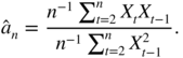
As an example, consider the least‐squares estimator ![]() of the parameter
a
in (A.1). By definition
of the parameter
a
in (A.1). By definition

From the first‐order condition, we obtain
The ergodic theorem shows that the numerator tends almost surely to
γ(1) = Cov(X
t
, X
t − 1) = aγ(0) and that the denominator tends to
γ(0). It follows that ![]() almost surely as
n → ∞. Note that this result still holds true when the assumption that
η
t
is a strong white noise is replaced by the assumption that
η
t
is a semi‐strong white noise, or even by the assumption that
η
t
is an ergodic and stationary weak white noise.
almost surely as
n → ∞. Note that this result still holds true when the assumption that
η
t
is a strong white noise is replaced by the assumption that
η
t
is a semi‐strong white noise, or even by the assumption that
η
t
is an ergodic and stationary weak white noise.
A.2. Martingale Increments
In a purely random fair game (for instance, A and B play ‘heads or tails’, A gives one dollar to B if the coin falls tails, and B gives one dollar to A if the coin falls heads), the winnings of a player constitute a martingale.
When (Y t ) t ∈ ℕ is said to be a martingale, it is implicitly assumed that ℱ t = σ(Y u , u ≤ t), that is, the σ ‐field generated by the past and present values.
A.3 Mixing
Numerous probabilistic tools have been developed for measuring the dependence between variables. For a finite‐variance process, elementary measures of dependence are the autocovariances and autocorrelations. When there is no linear dependence between X t and X t + h , as is the case for a GARCH process, the autocorrelation is not the right tool, and more elaborate concepts are required. Mixing assumptions, introduced by Rosenblatt (1956), are used to convey different ideas of asymptotic independence between the past and future of a process. We present here two of the most popular mixing coefficients.
A.3.1 α‐Mixing and β‐Mixing Coefficients
The strong mixing (or α ‐mixing) coefficient between two σ ‐fields 풜 and ℬ 3 is defined by
It is clear that
- (i) if
 and ℬ are independent then
  ;
; - (ii)
 ;
4
;
4
- (iii)
 provided that
  contains an event of probability 1/2;
 - (iv)
 provided that
  is non‐trivial;
5
is non‐trivial;
5
- (v)
 provided that
  and ℬ′ ⊂ ℬ.
The strong mixing coefficients of a process X = (X t ) are defined by
If
X
is stationary, the term ![]() can be omitted. In this case, we have
can be omitted. In this case, we have

where the first supremum is taken on A ∈ σ(X s , s ≤ 0) and B ∈ σ(X s , s ≥ h) and the second is taken on the set of the measurable functions f and g such that ∣f ∣ ≤ 1, ∣g ∣ ≤ 1. X is said to be strongly mixing, or α ‐mixing, if α X (h) → 0 as h → ∞. If α X (h) tends to zero at an exponential rate, then X is said to be geometrically strongly mixing.
The β ‐mixing coefficients of a stationary process X are defined by

where in the last equality, the sup is taken among all the pairs of partitions {A
1, …, A
I
} and {B
1, …, B
J
} of Ω such that
A
i
∈ σ(X
s
, s ≤ 0) for all
i
and
B
j
∈ σ(X
s
, s ≥ k) for all
j
. The process is said to be
β
‐mixing if ![]() . We have
. We have
so that β ‐mixing implies α ‐mixing. If Y = (Y t ) is a process such that Y t = f(X t , …, X t − r ) for a measurable function f and an integer r ≥ 0, then σ(Y t , t ≤ s) ⊂ σ(X t , t ≤ s) and σ(Y t , t ≥ s) ⊂ σ(X t − r , t ≥ s). In view of point (v) above, this entails that
A.3.2 Covariance Inequality
Let p, q , and r be three positive numbers such that p −1 + q −1 + r −1 = 1. Davydov (1968) showed the covariance inequality
where ![]() and
K
0
is a universal constant. Davydov initially proposed
K
0 = 12. Rio (1993) obtained a sharper inequality, involving the quantile functions of
X
and
Y
. The latter inequality also shows that one can take
K
0 = 4 in (A.8). Note that (A.8) entails that the autocovariance function of an
α
‐mixing stationary process (with enough moments) tends to zero.
and
K
0
is a universal constant. Davydov initially proposed
K
0 = 12. Rio (1993) obtained a sharper inequality, involving the quantile functions of
X
and
Y
. The latter inequality also shows that one can take
K
0 = 4 in (A.8). Note that (A.8) entails that the autocovariance function of an
α
‐mixing stationary process (with enough moments) tends to zero.
A.3.3 Central Limit Theorem
Herrndorf (1984) showed the following CLT.