12
Parameter‐Driven Volatility Models
In this chapter, we consider volatility models in which the volatility no longer coincides with the conditional variance. In other words, volatility would remain unobservable even if the parameters of the data‐generating process were known. Such models are naturally related to GARCH and can be seen as their competitors/alternatives in financial applications.
The difference between the different volatility modellings can be perceived through the concepts of observation‐driven and parameter‐driven models introduced by Cox (1981) and recently revisited by Koopman, Lucas and Scharth (2016). Suppose that φ t is a ‘parameter’ at time t . Let ε t be an observed random variable at time t . In an observation‐driven model,
where Φ is a measurable function. In a parameter‐driven model,
where ![]() is an idiosyncratic innovation at time
t
and Φ*
is a measurable function. In the latter case, there is a latent structure in the model which, in general, cannot be directly related to the observations.
is an idiosyncratic innovation at time
t
and Φ*
is a measurable function. In the latter case, there is a latent structure in the model which, in general, cannot be directly related to the observations.
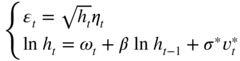
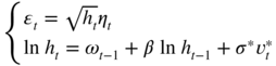
Let us a consider a GARCH model, choosing the volatility for the parameter: φ t = σ t . Under stationarity and invertibility conditions, σ t can be expressed as a function of the past observations, making the model observation‐driven. This enables to write the likelihood function easily, for any purported distribution of the innovation η t . Most GARCH models can also be considered as parameter‐driven since, for instance, in the GARCH(1,1) case,
We will focus in this chapter on two classes of volatility models – the stochastic volatility (SV) and the Markov switching GARCH models – which do not have an observation‐driven form, but can be given a parameter‐driven representation.
12.1 Stochastic Volatility Models
In GARCH models, the concepts of conditional variance and volatility coincide. By making volatility a function of the past observations, these specifications are particularly convenient for statistical purposes and are amenable to multivariate extensions. However, they may be difficult to study from a probability point of view and may imply important dynamic restrictions. 1
By contrast, in the so‐called SV models, volatility is a latent variable which cannot be expressed as a function of observable variables and satisfies a dynamic model. The observed process, ε t , and its volatility, σ t , are still related by the equation
where (η t ) is a strong white noise sequence, which may or may not be independent from the process (σ t ). The model is completed by specifying a dynamic for σ t , which only has to be compatible with the positivity of σ t .
Contrary to GARCH models – for which a plethora of formulations have been developed, and which can be used with different orders like ARMA models – a prominent part of the literature on SV models focused on a simple first‐order specification, often considered sufficient to capture the main characteristics of financial series. This specification – called the canonical SV model – postulates an AR(1) model for the dynamics of ![]() . While the probability structure is much simpler, the statistical inference is much more complex than in GARCH models, which has refrained practitioners from considering SV as a benchmark model for financial data.
. While the probability structure is much simpler, the statistical inference is much more complex than in GARCH models, which has refrained practitioners from considering SV as a benchmark model for financial data.
12.1.1 Definition of the Canonical SV Model
The canonical SV model is defined by

where (η
t
) and (![]() ) are two independent sequences of iid zero‐mean and unit‐variance random variables,
ω, β
and
σ
are parameters.
) are two independent sequences of iid zero‐mean and unit‐variance random variables,
ω, β
and
σ
are parameters.
Under conditions ensuring the existence of a solution, the variable ![]() is called the volatility of
ε
t
. As in GARCH models, the magnitude of
ε
t
is proportional to
is called the volatility of
ε
t
. As in GARCH models, the magnitude of
ε
t
is proportional to ![]() , and the sign of
ε
t
is independent from
, and the sign of
ε
t
is independent from ![]() and from any past variable. Dependence between
ε
t
and its past values is introduced indirectly, through the log‐volatility dynamics. However, contrary to what occurs with GARCH‐type models, the volatility at time
t
cannot be interpreted as the conditional variance of
ε
t
.
2
Another difference with GARCH specifications is that, by specifying an AR(1) dynamics on the log‐volatility rather than on the volatility, the parameters
ω
,
β
, and
σ
are a priori free of positivity constraints. Such constraints have nevertheless to be introduced to ensure either identifiability of the parameters, or sensible interpretation and compatibility with the data.
and from any past variable. Dependence between
ε
t
and its past values is introduced indirectly, through the log‐volatility dynamics. However, contrary to what occurs with GARCH‐type models, the volatility at time
t
cannot be interpreted as the conditional variance of
ε
t
.
2
Another difference with GARCH specifications is that, by specifying an AR(1) dynamics on the log‐volatility rather than on the volatility, the parameters
ω
,
β
, and
σ
are a priori free of positivity constraints. Such constraints have nevertheless to be introduced to ensure either identifiability of the parameters, or sensible interpretation and compatibility with the data.
Parameter
β
plays the role of a persistence coefficient. Indeed, when
β
is close to 1, a positive shock on the log‐volatility (due to a large positive value of ![]() ) has a persistent effect on
h
t
: the volatility will remain high over several dates. A negative shock on the log‐volatility, implying a small level for the volatility
h
t
, is also persistent when
β
is close to 1. If
β
is close to 0, the effect of large shocks vanishes rapidly. Now if
β
is close to –1, the instantaneous effect of a positive shock is a large volatility, but at the next period, this volatility takes a small value, and subsequently oscillates between large and small values provided no other big shock occurs. A negative shock produces the same kind of alternate effects. Such behaviours being rarely observed on financial series, negative values of
β
can be considered unrealistic for applications.
) has a persistent effect on
h
t
: the volatility will remain high over several dates. A negative shock on the log‐volatility, implying a small level for the volatility
h
t
, is also persistent when
β
is close to 1. If
β
is close to 0, the effect of large shocks vanishes rapidly. Now if
β
is close to –1, the instantaneous effect of a positive shock is a large volatility, but at the next period, this volatility takes a small value, and subsequently oscillates between large and small values provided no other big shock occurs. A negative shock produces the same kind of alternate effects. Such behaviours being rarely observed on financial series, negative values of
β
can be considered unrealistic for applications.
The interpretation of the other coefficients is more straightforward. Parameter
ω
is a scale factor for the volatility. The canonical SV model is clearly stable by scaling: if the returns
ε
t
are multiplied by some constant
c
, then the process ![]() satisfies the same SV model, except for the coefficient
ω
which is replaced by
satisfies the same SV model, except for the coefficient
ω
which is replaced by ![]() . Finally, parameter
σ
can be interpreted as the volatility of the log‐volatility. Without generality loss, it can be assumed that
σ ≥ 0.
. Finally, parameter
σ
can be interpreted as the volatility of the log‐volatility. Without generality loss, it can be assumed that
σ ≥ 0.
One motivation for considering the SV model is that it can be interpreted as the discretised version of diffusion models used in finance. For instance, a popular continuous‐time model for the asset price S t is given by

where (W 1t ) and (W 2t ) are independent Brownian motions. In this model, the log‐volatility follows an Ornstein–Uhlenbeck process. The canonical SV model – with an intercept μ added in the equation of ε t = log(S t /S t − 1) – can be seen as a discrete‐time version of the previous continuous‐time model.
12.1.2 Stationarity
The probabilistic structure of the SV model is much simpler than that of GARCH models. Indeed, the stationarity of the volatility sequence (h
t
) in Model (12.1) can be studied independently from the iid sequence (η
t
). Call non‐anticipative any solution (ε
t
) of Model ( 12.1) such that
ε
t
belongs to
σ{(η
u
, ![]() ) : u ≤ t}. The proof of the following result is immediate.
) : u ≤ t}. The proof of the following result is immediate.
The second‐order properties of the strictly stationary solution can be summarised as follows (see Exercise 12.1 for a proof). Let
Kurtosis of the Marginal Distribution
In view of ( 12.3), the existence of a fourth‐order moment for ε t requires the conditions

We then have

and the kurtosis coefficient of the marginal distribution of ε t is given by

where
κ
η
is the kurtosis coefficient of
η
t
and
κ
(i)
is the kurtosis coefficient of ![]() . Because the law of
. Because the law of ![]() is non‐degenerate,
κ
(i) > 1. Thus, the kurtosis of the marginal distribution is strictly larger than that of the conditional distribution of
ε
t
. When
is non‐degenerate,
κ
(i) > 1. Thus, the kurtosis of the marginal distribution is strictly larger than that of the conditional distribution of
ε
t
. When ![]() , we have
, we have ![]() In particular if we also have
In particular if we also have ![]() , then the distribution of
ε
t
is leptokurtic (
κ
ε
> 3).
, then the distribution of
ε
t
is leptokurtic (
κ
ε
> 3).
Tails of the Marginal Distribution
When stable laws are estimated on series of financial returns, one generally obtains heavy‐tailed marginal distributions. 4 It is, therefore, useful to study in more detail the tail properties of the marginal distribution of SV processes. We relax in this section the assumption of finite variance for η t .
The distribution of a non‐negative random variable X is said to be regularly varying with index α , which can be denoted X ∈ RV(α) if
with α ∈ (0, 2) and L(x) a slowly varying function at infinity, which is defined by the asymptotic relation L(tx)/L(x) → 1 as x → ∞, for all t > 0. 5 If X satisfies (12.5), then E(X r ) = ∞ for r > α and E(X r ) < ∞ for r < α (for r = α , the expectation may be finite or infinite, depending on the slowly varying function L ). To handle products, the following result by Breiman (1965, Eq. (3.1)) can be useful: for any non‐negative independent random variables X and Y , where X ∈ RV(α) and E(Y α + δ ) < ∞ for some δ > 0, we have
It follows that if, in Model ( 12.1) without the assumption that ![]() , ∣η
t
∣ ∈ RV(α), and if the noise (υ
t
) is such that
, ∣η
t
∣ ∈ RV(α), and if the noise (υ
t
) is such that ![]() , for some
τ > 0, then
ε
t
inherits the heavy‐tailed property of the noise (η
t
). This is in particular the case if (υ
t
) is Gaussian, since
h
t
then admits moments at any order.
, for some
τ > 0, then
ε
t
inherits the heavy‐tailed property of the noise (η
t
). This is in particular the case if (υ
t
) is Gaussian, since
h
t
then admits moments at any order.
12.1.3 Autocovariance Structures
Under the conditions of Theorem 12.2, the SV process (ε t ) is uncorrelated yet dependent. In other words, like GARCH processes, it is not white noise in the strong sense. As for GARCH models, the dependence structure of (ε t ) can be studied through the autocorrelation function of appropriate transformations of the SV process.
ARMA Representation for 
Assuming
P(η
t
= 0) = 0, and by taking the logarithm of ![]() , the first equation of ( 12.1) writes as follows:
, the first equation of ( 12.1) writes as follows:
This formulation allows us to derive the autocovariance function of the process ![]() . Let
. Let ![]() Assume that
Z
t
admits fourth‐order moments, and let
μ
Z
= E(Z
t
),
Assume that
Z
t
admits fourth‐order moments, and let
μ
Z
= E(Z
t
), ![]() , and
, and ![]() 6
The next result (see Exercise 12.3 for a proof) shows that (X
t
) admits an ARMA representation.
6
The next result (see Exercise 12.3 for a proof) shows that (X
t
) admits an ARMA representation.
Note that, in Eq. (12.7), the noise (u t ) is not strong. This sequence is not even a martingale difference sequence (unlike the noise of the ARMA representation for the square of a GARCH process). This can be seen by computing, for instance,
Even when (![]() ) is symmetrically distributed, this quantity is generally non‐zero. This shows that
u
t
is correlated with some (non‐linear) functions of its past: thus
E(u
t
∣ u
t − 1, u
t − 2, …) ≠ 0 (a. s.).
) is symmetrically distributed, this quantity is generally non‐zero. This shows that
u
t
is correlated with some (non‐linear) functions of its past: thus
E(u
t
∣ u
t − 1, u
t − 2, …) ≠ 0 (a. s.).
Autocovariance of the Process 
When the process ![]() is second‐order stationary, that is under Eq. (12.4), deriving its autocovariance function has interest for comparison with GARCH models and for statistical applications.
is second‐order stationary, that is under Eq. (12.4), deriving its autocovariance function has interest for comparison with GARCH models and for statistical applications.
Using Eq. ( 12.3) we get, for all k ≥ 0

For
k > 0, since ![]() and
and ![]() are independent and have unit expectation,
are independent and have unit expectation,

where, for
i ≥ k
,
α
k, i
= E[exp{σβ
i
(1 + β
k
)
![]() }]. Thus, we have, for all
k > 0
}]. Thus, we have, for all
k > 0

Now suppose that ![]() . It follows that
. It follows that ![]() , and thus the second‐order stationarity condition reduces to
, and thus the second‐order stationarity condition reduces to ![]() and ∣β ∣ < 1 in this case. Therefore, for any
k > 0
and ∣β ∣ < 1 in this case. Therefore, for any
k > 0

It can be noted that the autocovariance function of ![]() tends to zero when
k
goes to infinity, but that the decreasing is not compatible with a linear recurrence equation on the autocovariances. In other words, the process
tends to zero when
k
goes to infinity, but that the decreasing is not compatible with a linear recurrence equation on the autocovariances. In other words, the process ![]() – though second‐order stationary and admitting a Wold representation – does not have an ARMA representation. However, we have an equivalent of the form
– though second‐order stationary and admitting a Wold representation – does not have an ARMA representation. However, we have an equivalent of the form ![]() as
k → ∞, which shows that the asymptotic (exponential) rate of decrease of the autocovariances is the same as for an ARMA process. Recall that, by contrast, squared fourth‐order stationary GARCH processes satisfy an ARMA model.
as
k → ∞, which shows that the asymptotic (exponential) rate of decrease of the autocovariances is the same as for an ARMA process. Recall that, by contrast, squared fourth‐order stationary GARCH processes satisfy an ARMA model.
12.1.4 Extensions of the Canonical SV Model
Many other specifications could be considered for the volatility dynamics. Obviously, the memory of the process could be extended by introducing more lags in the AR model, that is an AR( p ) instead of an AR(1). An insightful extension of model ( 12.1) is obtained by allowing a form of dependence between the two noise sequences. We consider two natural extensions of the basic model.
Contemporaneous Correlation
A contemporaneous correlation coefficient ρ between the disturbances of model ( 12.1) is introduced by assuming that (η t , υ t ) forms an iid centred normal sequence with Var(η t ) = Var(υ t ) = 1 and Cov(η t , υ t ) = ρ . The model can thus be equivalently written as
where
ω
t
= ω + σρη
t
, ![]() , (η
t
) and
, (η
t
) and ![]() are two independent sequences of iid normal variables with zero mean and variance equal to 1. We still assume that ∣β ∣ < 1, which ensures stationarity of the solution (ε
t
) defined in ( 12.3). If the correlation
ρ
is negative, a negative shock on the price – corresponding to a negative
η
t
– is likely to be associated with an increase of the volatility at the current date and – if
β > 0 – at the subsequent dates. Conversely, a positive shock on the price –
η
t
> 0 – is likely to be compensated by a decrease of the volatility. The contemporaneous correlation between the iid processes of the SV model thus induces asymmetry effects, similar to the leverage effect described in Chapter 1. This effect, characterised by a negative correlation between the current price and the future volatility, has been often detected in stock prices. However, the correlation coefficient
ρ
also entails a non‐zero mean
are two independent sequences of iid normal variables with zero mean and variance equal to 1. We still assume that ∣β ∣ < 1, which ensures stationarity of the solution (ε
t
) defined in ( 12.3). If the correlation
ρ
is negative, a negative shock on the price – corresponding to a negative
η
t
– is likely to be associated with an increase of the volatility at the current date and – if
β > 0 – at the subsequent dates. Conversely, a positive shock on the price –
η
t
> 0 – is likely to be compensated by a decrease of the volatility. The contemporaneous correlation between the iid processes of the SV model thus induces asymmetry effects, similar to the leverage effect described in Chapter 1. This effect, characterised by a negative correlation between the current price and the future volatility, has been often detected in stock prices. However, the correlation coefficient
ρ
also entails a non‐zero mean
and non‐zero autocorrelations for the process (ε t ) which, in financial applications, is often inappropriate (see Exercise 12.4). Therefore, it appears that the correlation coefficient ρ has several roles in this model, which makes it difficult to interpret.
Leverage Effect
A non‐contemporaneous correlation between the disturbances of model ( 12.1) allows to pick up the leverage effect, without removing the zero‐mean property. Therefore, we assume that (η t − 1, υ t ) forms an iid centred normal sequence with Var(η t ) = Var(υ t ) = 1 and Cov(η t − 1, υ t ) = ρ . The model is given by
with the same notations as in the last section. By ( 12.3), we have E(ε t ) = 0 and Cov(ε t , ε t − k ) = 0 for k > 0. Thus, the white noise property of the stationary solution is preserved with this correlation structure of the two disturbances sequences.
Intuitively, when
ρ < 0, a large negative shock on the noise
η
at time
t − 1 – that is, a sudden price fall – is likely to produce (through the correlation between ![]() and
η
t − 1
) a large volatility at the next period (and at the subsequent ones if
β > 0). The following result shows that the model is indeed able to capture the leverage effect and provides a quantification of this effect.
and
η
t − 1
) a large volatility at the next period (and at the subsequent ones if
β > 0). The following result shows that the model is indeed able to capture the leverage effect and provides a quantification of this effect.
To summarise, the SV model where η t − 1 and υ t are negatively correlated is able to capture the leverage effect, while preserving the white noise property of (ε t ). As the horizon increases, however, this effect is maintained only if β > 0 and it vanishes exponentially.
12.1.5 Quasi‐Maximum Likelihood Estimation
Estimating parameters in a SV model – even in the simple canonical SV model – is a difficult task because the volatility process is latent. In GARCH‐type models, the period‐ t volatility is also non‐observed, but it only depends on (i) unknown parameters, and (ii) the sample path of the (observed) returns process up to time t − 1. It follows that the log‐likelihood can be written in closed‐form for all invertible GARCH models. Because the log‐likelihood cannot be explicitly written for SV models, a plethora of alternative methods have been suggested. To mention just a few, the following approaches can be used: the Kalman filter, Generalised Moments Methods (GMM), simulations‐based methods (in particular Bayesian Markov chain Monte Carlo (MCMC) methods). We will limit ourselves to the Kalman filter method (see Appendix D for a general presentation) of evaluating the likelihood. Although this method may be numerically less accurate than more sophisticated ones, it is easy to implement, computationally fast, and amenable to extensions – in particular multivariate extensions – of the SV model.
The state‐space form of model ( 12.1) is straightforwardly obtained by taking logarithms:

using the notations of Section 12.1.3.
Applying the Kalman filter is not without difficulty in this framework, because it requires assuming a Gaussian distribution for ![]() . For financial returns, the marginal distributions are known to be heavy tailed. Even if the relation between such marginal distributions and the distribution of
. For financial returns, the marginal distributions are known to be heavy tailed. Even if the relation between such marginal distributions and the distribution of ![]() is complex, it seems unrealistic to assume a normal distribution for
is complex, it seems unrealistic to assume a normal distribution for ![]() . As mentioned in Appendix D, when the normal assumption is in failure, the Kalman filter does not provide the exact conditional variance of the observed process, but rather an approximation.
. As mentioned in Appendix D, when the normal assumption is in failure, the Kalman filter does not provide the exact conditional variance of the observed process, but rather an approximation.
Let
The algorithm described in Appendix D takes here a simplified form:
In view of Proposition D.1 in Appendix D, if ∣β ∣ < 1 the sequence (P t ∣ t − 1) converges. The limit P * is obtained as the unique positive solution of the Ricatti equation (D.22), that is
One can easily check that ∣P t ∣ t − 1 − P * ∣ < β 2 ∣ P t − 1 ∣ t − 2 − P *∣, the rate of convergence is thus exponential.
Finally, the log‐likelihood writes:

For fixed values of
μ
Z
and ![]() , parameter θ = (ω, β, σ) can thus be estimated by maximising this function, which is built by applying the previous algorithm. It can be noted that the conditional variance
F
t ∣ t − 1
obtained by this algorithm does not depend on the observations.
, parameter θ = (ω, β, σ) can thus be estimated by maximising this function, which is built by applying the previous algorithm. It can be noted that the conditional variance
F
t ∣ t − 1
obtained by this algorithm does not depend on the observations.
12.2 Markov Switching Volatility Models
When GARCH models are fitted over sub‐periods of long time series of returns, one often find important differences in estimated parameters (see Exercise 12.5). This discrepancy can be interpreted as the indication that the dynamics is changing over time. Such dynamic changes are not surprising given the existence of business cycles in the economy, characterised by well‐known phases/regimes of recession, depression, recovery, and expansion. A natural way to model changes in regime is to postulate the existence of an underlying latent 7 variable of regime change, taking values in a finite set and satisfying – for simplicity – the Markov property.
Models constructed with a latent Markov chain have found widespread applications in various domains including economics, biology, finance, and speech recognition. We start by presenting a class of Hidden Markov Models (HMM), which can be seen as dynamic extensions of finite mixture models.
12.2.1 Hidden Markov Models
A process (ε t ) t ≥ 0 satisfies a HMM if
- conditional on some unobserved Markov chain (Δ t ), the (observed) variables ε 0, ε 1, … are independent;
- the conditional law of ε s given (Δ t ) only depends on Δ s .
For instance, the observed and latent processes can be related through the multiplicative model

where
(η t ) is a sequence of iid centred variables with unit variance, and Δ t is a Markov chain on ℰ = {1,…, d}. Set ℰ is called the set of states, or regimes, of the Markov chain (see Appendix C for basic elements of the Markov Chain theory). The transition matrix is denoted by ℙ. It is assumed that:
- A1 The Markov chain (Δ t ) is stationary, irreducible and aperiodic.
- A2 The processes (η t ) and (Δ t ) are independent.
Note that the condition (12.16) is not restrictive because if ω(i) = ω(j), the states i and j can be merged by changing the Markov chain. This model is pertinent for financial returns, as it belongs to the general class of random conditional variance models defined in (1.6), where ℱ t − 1 is the σ ‐field generated by the random variable Δ t . Although very simple, this model presents strong similarities – but also noticeable differences – with standard GARCH models.
Comparison with GARCH Models
As in GARCH or SV models, the observed process (ε
t
) is centred and its sample paths fluctuate around zero. The magnitude of the fluctuations will be different according to the state of the Markov chain Δ
t
. Regime 1 is characterised by small fluctuations, while regime
d
is associated with the most turbulent periods. The length of stay in a given regime, as well as the number of transitions from one regime to another only depend on the transition probabilities of the Markov chain. An example of sample path (100 observations) is displayed in Figure 12.1. The path is simulated from a three‐regime model with ![]() and
and


Figure 12.1
Simulation of length 100 of a three‐regime HMM. The full line corresponds to the simulated values of
ε
t
and the dotted lines correspond to  . Source: Francq and Roussignol (1997).
This very simple model presents similarities with GARCH‐type models. By construction, the clustering property 8 is satisfied.
The assumptions made on the Markov chain and on ( η t ) entail that any solution of model (12.15) is obviously strictly stationary. Moments of ε t exist at any order, provided that the same moments exist for η t . By the independence between η t and Δ t , we have for any real positive number r ,

In particular, ε t is centred. Recall that for GARCH processes, moments cannot exist at any order. Although the marginal distribution of ε t does not possess heavy‐tails, the leptokurticity property is satisfied in the HMM: the law of ε t has fatter tails than that of η t . If a Gaussian distribution is assumed for η t , the Kurtosis coefficient of ε t is strictly greater than 3 (the exact value depends on both the transition probabilities of the chain and the values of the variances ω(i) in the different regimes).
An important difference with GARCH model pops up when we compute the conditional Kurtosis coefficient. Recall that this coefficient is constant for GARCH‐type models. For model ( 12.15) we have

and no simplification occurs here, because ![]() is not a function of past values of
ε
t
. Thus, the shape of the conditional distribution – not only the variance – may also fluctuate over time.
is not a function of past values of
ε
t
. Thus, the shape of the conditional distribution – not only the variance – may also fluctuate over time.
Less straightforward similarities with standard GARCH models appear by studying the autocorrelation functions of (ε
t
) and ![]() .
.
Autocorrelations, Moments
We have
hence (ε t ) is a white noise with variance

We now study the autocorrelation of the squared process. For ease of presentation, let us first consider the case where
d = 2. The eigenvalues of the transition matrix are 1 and
λ ≔ p(1, 1) + p(2, 2) − 1, since the Markov chain is, by assumption A1, irreducible and aperiodic. Note that −1 < λ < 1. By diagonalising ℙ, it can easily be seen that the entries of ℙ
k
have the form
p
(k)(i, j) = a
1(i, j) + a
2(i, j)λ
k
, for
k ≥ 0. By letting
k
go to infinity, we get
a
1(i, j) = π(j) and, using the value
k = 0:
a
1(i, j) + a
2(i, j) = ![]() {i = j}. It follows that for
j = 1, 2 and
i ≠ j
{i = j}. It follows that for
j = 1, 2 and
i ≠ j
hence, for i, j = 1, 2
We have, for k > 0,

and thus, by using Eq. (12.17),

It is worth noting that the autocorrelations of the squares decrease at exponential rate like for a second‐order stationary GARCH process. An important difference, however, is that the rate of this convergence is not related to the existence of moments. Note also that the larger ∣λ ∣ = ∣ 1 − p(1, 1) − p(2, 2)∣, the slower the decrease of the autocorrelations (in module). In other words, the autocorrelations decrease slowly when the transition probabilities from a regime to the other are either both very small or both close to 1. Obviously, ![]() for any
k > 0 when
ω(1) = ω(2) because
ε
t
is an iid white noise in this case. A similar computation shows that
for any
k > 0 when
ω(1) = ω(2) because
ε
t
is an iid white noise in this case. A similar computation shows that
We deduce from Eqs. (12.19) and (12.20) that ![]() admits an ARMA(1,1) representation, with autoregressive coefficient
λ
.
admits an ARMA(1,1) representation, with autoregressive coefficient
λ
.
In the general case, matrix ℙ may not be diagonalisable but has an eigenvalue equal to 1, with corresponding eigenspace of dimension 1. Denote by λ 1,…, λ m the other eigenvalues and n 1,…, n m the dimensions of the corresponding eigenspaces ( n 1 + ⋯ + n m = d − 1). The Jordan form of matrix ℙ is ℙ = SJS −1 , where S is non‐singular and

with
J
l
(λ) = λ핀
l
+ N
l
(1), denoting by
N
l
(i) the square matrix of dimension
l
whose entries are equal to zero, except for the
i
th uperdiagonal whose elements are equal to 1. Using ![]() for
k
′ ≤ l − 1 and
for
k
′ ≤ l − 1 and ![]() for
k
′ > l − 1, we get
for
k
′ > l − 1, we get

where P (l) is a polynomial of degree l − 1. It follows that

We deduce that
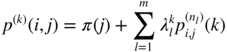
where the ![]() are polynomials of degree
n
l
− 1. The first term in the right‐hand side is identified by the convergence
p
(k)(i, j) → π(j) as
k → ∞. Note that ∣λ
l
∣ < 1 for
l = 1,…, m
. Finally, we have, using (12.18),
are polynomials of degree
n
l
− 1. The first term in the right‐hand side is identified by the convergence
p
(k)(i, j) → π(j) as
k → ∞. Note that ∣λ
l
∣ < 1 for
l = 1,…, m
. Finally, we have, using (12.18),

where the ![]() 's are polynomials of degree
n
l
− 1.
's are polynomials of degree
n
l
− 1.
The computation of ![]() is more tedious, but it can be shown that this expectation depends of
k
through the
is more tedious, but it can be shown that this expectation depends of
k
through the ![]() 's (similarly to (12.21)). Thus, the Markov chain (Δ
t
) introduces a source of persistence of shocks on the volatility.
's (similarly to (12.21)). Thus, the Markov chain (Δ
t
) introduces a source of persistence of shocks on the volatility.
Estimation
The vector of parameters of model ( 12.15) is
The likelihood can be written by conditioning on all possible paths (e 1,…, e n ) of the Markov chain, where the e i belong to ℰ = {1,…, d}. For ease of presentation, we assume a standard Gaussian distribution for η t but the estimation procedure can be adapted to other distributions. The probability of such paths is given by
For each path, we get a conditional likelihood of the form
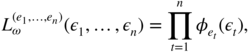
where
φ
i
(·) denotes the density of the law ![]() .
.
Finally, the likelihood writes
Unfortunately, this formula cannot be used in practice because the number of summands is d n , which is huge even for small samples and two regimes. For instance, 2300 is generally considered to be an upper bound for the number of atoms in the universe. 9 Several solutions to this numerical problem – computing the likelihood – exist.
Computing the Likelihood
Matrix Representation
Let
where g k (· ∣ Δ k = i) is the law of (ε 1,…, ε k ) given {Δ k = i}. One can easily check that
and

In matrix form we get
where

Hence, letting ![]() , we have
, we have
which is computationally usable (with an order of d 2 n multiplications).
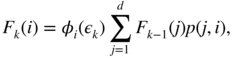
Forward–Backward Algorithm
Let B k (i) = B k (ε k + 1,…, ε n ∣ Δ k = i) the law of (ε k + 1,…, ε n ) given {Δ k = i}. By the Markov property, we have
The Forward formulas, allowing us to compute F k (i) for k = 1, 2, … , are given by (12.22) and (12.23). The Backward formulas, allowing us to compute B k (i) for k = n − 1, n − 2, … are

We thus obtain

for any k ∈ {1,…, n}. For k = n , we retrieve Eq. (12.24).
Hamilton Filter
The Forward–Backward algorithm was developed in the statistical literature (Baum 1972). Models involving a latent Markov chain were put forward in the econometric literature by Hamilton (1989). Let

φ(ε t ) = (φ 1(ε t ),…, φ d (ε t ))′ , and denote by ⊙ the element‐by‐element Hadamard product of matrices.
With obvious notations, we get

where

Starting from an initial value π 1 ∣ 0 = π (the stationary law) or π 1 ∣ 0 = π 0 (a given initial law), we can compute
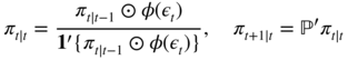
for t = 1,…, n , and we deduce the conditional log‐likelihood

where
The Hamilton algorithm (12.29)–(12.31) seems numerically more efficient than the Forward–Backward algorithm in ( 12.22)–( 12.23) and (12.26)–(12.28) which, under this form, produces underflows. Note, however, that conditional versions of the Forward–Backward algorithm have been developed to avoid this problem (Devijver 1985). Note also that the matrix formulation (12.25) is very convenient for establishing asymptotic properties of the ML estimator (see Francq and Roussignol 1997).
Maximising the Likelihood
Maximisation of the (log‐)likelihood can be achieved by a classical numerical procedure, or using the EM (Expectation–Maximisation) algorithm, which can be described as follows.
For ease of exposition, we consider that the initial distribution π 0 (the law of Δ1 ) is not necessarily the stationary distribution π . In the EM algorithm, π 0 is an additional parameter to be estimated. If – in addition to (ε 1,…, ε n ) – one could also observe (Δ1,…, Δ n ), estimating θ and π 0 by ML would be an easy task. Indeed,
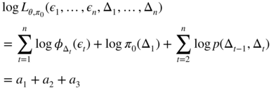
where


From (12.32), we need to maximise the terms ![]() with respect to
ω(i), for
i = 1,…, d
. This yields the estimators
with respect to
ω(i), for
i = 1,…, d
. This yields the estimators

Maximisation of (12.33) with respect to
π
0(1),…, π
0(d), under the constraint ![]() , yields
, yields
From (12.34), for
i = 1,…, d
, one has to maximise with respect to
p(i, 1),…, p(i, d), under the constraint ![]() , the sum
, the sum

We obtain 10

In practice, formulas (12.35), (12.36), and (12.37) cannot be used, because (Δ t ) is unobserved. Generally speaking, the EM algorithm alternates between steps E – for expectation – where the expectation of the likelihood is evaluated using the current value of the parameter, and steps M – for maximisation – where the objective function computed in step E is maximised. In the present setting, the EM algorithm only requires steps M, together with the computation of the predicted and filtered probabilities – π t ∣ t − 1 and π t ∣ t , respectively – of the Hamilton filter ( 12.29), and also an additional step for the computation of the smoothed probabilities.
Step E
Suppose that an estimator ![]() de (θ, π
0) is available. It seems sensible to approximate the unknown log‐likelihood by its expectation given the observations (ε
1,…, ε
n
), evaluated under the law parameterised by
de (θ, π
0) is available. It seems sensible to approximate the unknown log‐likelihood by its expectation given the observations (ε
1,…, ε
n
), evaluated under the law parameterised by ![]() . We get the criterion
. We get the criterion

where


Step M
We aim at maximising, with respect to (θ, π
0), the estimated log‐likelihood ![]() . Maximisation of (12.38) yields the solution
. Maximisation of (12.38) yields the solution

The estimated variance of regime
i
is thus a weighted mean of the ![]() , where the weights are the conditional probabilities that the chain lie in state
i
at time
t
. Similarly, (12.39) yields
, where the weights are the conditional probabilities that the chain lie in state
i
at time
t
. Similarly, (12.39) yields
and (12.40) yields

Formulas (12.41), (12.42), and (12.43) require computation of the smoothed probabilities
and
Computation of Smoothed Probabilities
The Markov property entails that, given Δ t , the observations ε t , ε t + 1, … do not convey information on Δ t − 1 . We hence have
and

It remains to compute the smoothed probabilities π t ∣ n , given by

for
t = n, n − 1,…, 2. Starting from an initial value ![]() , formulas ( 12.41), ( 12.42), and ( 12.43) allow us to obtain a sequence of estimators
, formulas ( 12.41), ( 12.42), and ( 12.43) allow us to obtain a sequence of estimators ![]() which increase the likelihood (see Exercise 12.13).
which increase the likelihood (see Exercise 12.13).
Summary of the Algorithm
Starting from initial values for the parameters

the algorithm consists in
repeating the following steps until consistency:
-
Setπ 1 ∣ 0 = π 0and
-
Compute the smoothed probabilitiesπ t ∣ n (i) = P(Δ t = i ∣ ε 1,…, ε n )using
andπ t − 1, t ∣ n (i, j) = P(Δ t − 1 = i, Δ t = j ∣ ε 1,…, ε n )from
-
Replace the previous values of the parameters byπ 0 = π 1 ∣ n ,
In practice, the sequence converges rather rapidly to the ML estimator (see the illustration below) if an appropriate starting value θ (0) > 0 is chosen (see Exercise 12.9).
Model ( 12.15) is certainly too simple to take into account, in their complexity, the dynamic properties of real‐time series (for instance of financial returns): whenever the series remain in the same regime, the observations have to be independent, and this assumption is quite unrealistic. A natural extension of model ( 12.15) – and also of the standard GARCH model – is obtained by assuming that, in each regime, the dynamics is governed by a GARCH model.
12.2.2 MS‐GARCH(p, q) Process
Consider the Markov–Switching GARCH (MS‐GARCH) process:

with the positivity constraints:
The model has d different GARCH regimes, which entails great flexibility. The standard GARCH – obtained for d = 1 – and the HMM – obtained when the α i (k)'s and β j (k)s are equal to zero – are particular cases of model (12.44).
Many properties highlighted for model ( 12.15) also hold for this general formulation. An important difference, however, is that the present model displays two distinct sources of persistence: one is conveyed by the chain (Δ t ), and the other one by the coefficients α i (·) and β j (·). For instance, regimes where shocks on past variables are very persistent may coexist with regimes where shocks are not persistent.
Another difference concerns the second‐order stationarity properties. To ensure that ε t admits a finite, time‐independent, variance in model ( 12.44), constraints on the coefficients α i (·) and β j (·), as well as on the transition probabilities, have to be imposed. Without entering into details, 11 note that the local stationarity – i.e. stationarity within each GARCH regime – is sufficient but not necessary for the global stationarity: a stationary solution of model ( 12.44) may have explosive GARCH regimes, provided that the transition probabilities towards such regimes are small enough. It is also worth noting that when only the intercept ω(·) is switching (i.e. when the α i 's and β j 's do not depend on Δ t ), we retrieve the usual second‐order stationarity condition (∑ i α i + ∑ j β j < 1). Finally, note that as in standard GARCH, once the existence Var(ε t ) is ensured, (ε t ) is a white noise.
Applications of MS‐GARCH models are often limited to MS‐ARCH. This restriction enables ML estimation with the Hamilton filter, as described in the previous section.
Illustration
For the sake of illustration, consider the CAC 40 and SP 500 stock market indices. Observations cover the period from March 1, 1990, to December 29, 2006. On the daily returns (in %), we fitted the HMM ( 12.15) and ( 12.16) with d = 4 regimes, using the R code given in Exercise 12.8. Taking initial values with non‐zero transition probabilities (see Exercise 12.9), after roughly 60 iterations of the EM algorithm, we obtain the following estimated model for the SP 500 series

and for the CAC 40

The estimated probabilities of the regimes are
and the average durations of the four regimes – given by 1/{1 − p(i, i)} – are approximately
Thus, the CAC stays in average 27 days in the more volatile regime, namely Regime 4. Figure 12.2 confirms that for the two series, the more volatile regime is also the less‐persistent regime, with however a long period of high volatility of 81 days (from June 27, 2002 to October 21, 2002) for the SP, and of 113 days (from June 4, 2002 to November 8, 2002) for the CAC. It is interesting to note that for the model of the SP 500, the possible transitions are always from one regime to an adjacent regime. Being, for instance in Regime 2, the chain can stay in Regime 2 or move to Regime 1 or 3, but the probability p(2, 4) of moving directly to Regime 4 is approximately zero. On the contrary, the CAC displays sudden moves from Regime 2 to Regime 4.
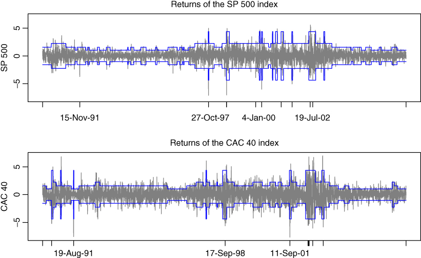
Figure 12.2 CAC 40 and SP 500 from March 1, 1990 to December 29, 2006, with ±2 times the standard deviation of the regime with the highest smoothed probability.
Conclusion
Estimation of GARCH‐type models over long time series, as those encountered in finance (i.e. typically several thousands of observations), generally produces strong volatility persistence. This effect may be spurious and may be explained by the need to obtain heavy‐tailed marginal distributions.
MS‐GARCH models enable to disentangle important properties of financial time series: persistence of shocks, decreasing autocorrelations of the squared returns, heavy tailed marginal distributions, and time‐varying conditional densities. These models are appropriate for series over a long time period, with successions of phases corresponding to the different regimes. Of course, such models – despite their flexibility – remain merely approximations of the real data generation mechanisms. 12
12.3 Bibliographical Notes
A recent presentation and statistical analysis of parameter‐driven and observation‐driven models can be found in Koopman, Lucas, and Scharth (2016). Continuous‐time models with SV have been widely studied in the option pricing literature: see, for instance Hull and White (1987), Melino and Turnbull (1990) and, more recently, Aït‐Sahalia, Amengual, and Manresa (2015). Harvey, Ruiz, and Shephard (1994) pointed out that the canonical SV model can be studied using a state‐space form allowing to apply the Kalman filter. The existence of the ARMA(1,1) representation for the log‐squared return process was mentioned by Ruiz (1994), and it was used by Breidt and Carriquiry (1996) to obtain QML estimates. See Davis and Mikosch (2009b) for mixing and tail properties of general SV models.
Various approaches have been developed for estimating SV models. Generalised method of moments (GMM) type of estimators have been proposed, for instance by Taylor (1986), Andersen (1994) and Andersen and Sørensen (1996). In the same spirit, Francq and Zakoian (2006a) proposed an estimation method based on the existence of ARMA representations for powers of the logarithm of the observed process. The QML method has been advocated by Harvey, Ruiz, and Sentana (1992), Harvey, Ruiz, and Shephard (1994) and Ruiz (1994), among others. An approach which is closely related to the QML uses a mixture of Gaussian distributions to approximate the non‐Gaussian error in the observation equation of the state‐space form (see, Mahieu and Schotman 1998). Bayesian MCMC methods of inference were applied to SV models, in particular by Jacquier, Polson, and Rossi (1994, 2004) and Kim, Shephard, and Chib (1998) and by Chib, Nardia and Shepard (2002). The simulated maximum likelihood (SML) method, relying on simulation of the latent volatility conditional on available information, was proposed by Danielsson (1994); the likelihood can also be calculated directly using recursive numerical integration procedures, as suggested by Fridman and Harris (1998). Estimation of SV models with leverage has been studied by Harvey and Shephard (1996), Yu (2005), Omori et al. (2007), among others. See Taylor (1994), Shephard and Andersen (2009), Renault (2009), and Jungbacker and Koopman (2009) for overviews on SV models.
Estimation of HMM was initially studied by Baum and Petrie (1966) and Petrie (1969). They proved consistency and asymptotic normality of the ML estimator when the observations are valued in a finite set. Leroux (1992) showed the consistency, and Bickel, Ritov, and Ryden (1998) established asymptotic normality for general observations. A detailed presentation of the algorithms required for the practical implementation can be found in Rabiner and Juang (1986).
Markov switching models were introduced by Hamilton (1989). In this paper, Hamilton developed a filter which can be applied when the regimes are Markovian (as the MS‐AR or the MS‐ARCH). MS‐ARCH models were initially studied by Hamilton and Susmel (1994), Cai (1994) and Dueker (1997). Stationarity conditions for MS‐GARCH, as well as estimation results for the MS‐ARCH can be found in Francq, Roussignol, and Zakoïan (2001), and Francq and Zakoïan (2005). Papers dealing with Bayesian estimation of MS‐GARCH are Kaufmann and Frühwirth‐Schnatter (2002), Das and Yoo (2004), Henneke et al. (2011), and Bauwens, Preminger, and Rombouts (2010). See the books by Cappé, Moulines, and Ryden (2005), Frühwirth‐Schnatter (2006), and Douc, Moulines, and Stoffer (2014) for an exhaustive overview on MS models.
12.4 Exercises
12.1 (Second‐order stationarity of the SV model)
Prove Theorem 12.2.
- 12.2 (Logarithmic transformation of the squared returns in the SV model) (Logarithmic transformation of the squared returns in the SV model) Show that the logarithmic transformation in (12.6) entails no information loss when the distribution of η t is symmetric.
- 12.3 (ARMA representation for the log‐squared returns in the SV model) Prove Theorem 12.3.
- 12.4 (Contemporaneously correlated SV model) Show that the contemporaneously correlated SV process is not centred and is autocorrelated.
- 12.5 (Fitting GARCH on sub‐periods of the CAC index) Consider a long period of a stock market index (for instance the CAC 40 from March 1, 1990 to December 29, 2006). Fit a GARCH(1,1) model on the returns of the first half of the series, and another GARCH(1,1) on the last part of the series. Compare the two estimated GARCH models, for instance by bootstrapping the estimated models.
-
12.6 (Invariant law of Ehrenfest's model) This model has been introduced in physics to describe the heat exchanges between two systems. The model considers balls numbered 1 to d in two urns A and B. At the initial step 0, the balls are randomly distributed between the two urns (each ball has probability 1/2 to be in urn A). At step
n ≥ 1, a number i is picked randomly in {1,…, d}, and the ball numbered i is transferred to the other urn. Let Δ
n
the number of balls in urn A at step n. Show that Δ
n
is a Markov chain on
 which is irreducible and periodic. Provide the transition matrix. Show that the initial law is invariant. If, instead, the initial law is the Dirac mass at 0, show that
  does not exist where π
n
denotes the distribution of Δ
n
.
does not exist where π
n
denotes the distribution of Δ
n
. - 12.7 (Period of an irreducible Markov chain) Show that the states of an irreducible Markov chain have the same period.
- 12.8 (Implementation of the EM algorithm) Implement the EM algorithm of Section 12.2.1 (in R for example).
- 12.9 (Choice of the initial value for the EM algorithm) Suppose that in the EM algorithm, the initial values are such that p(i 0, j 0) = 0 for some i 0, j 0 ∈ {1,…, d}. What are the next updated values of p(i 0, j 0) in the algorithm?
- 12.10 (Strict stationarity of the MS‐GARCH) Give a condition for strict stationarity of the Markov‐switching GARCH(p, q) model ( 12.44).
- 12.11 (Strict stationarity of the MS‐GARCH(1,1)) Give an explicit condition for strict stationarity of the Markov‐switching GARCH(1, 1) model. Consider the ARCH(1) case.
- 12.12 (Stationarity of the GARCH(1,1) with independent regime changes) with independent regime changes) Consider a GARCH(1,1) model with independent regime changes, namely a model of the form ( 12.44), where (Δ t ) is an iid sequence. Give a condition for the existence of a second‐order stationary solution.
-
12.13 (Consistency of the EM algorithm) Let
 be a sequence of estimators obtained from the EM algorithm section. With some abuse of notation, let
  be the likelihood and
  the joint distribution of the observations and of (Δ1,…, Δ
n
). Show that
the joint distribution of the observations and of (Δ1,…, Δ
n
). Show that  is an increasing sequence.
 - 12.14 (Likelihood of a MS‐ARCH) Consider an ARCH( q ) with Markov‐switching regimes, i.e. ( 12.44) with p = 0. Show that the likelihood admits a matrix form similar to ( 12.25), and that the forward–backward algorithm ( 12.22)–( 12.23) and ( 12.26)–( 12.28) can be applied, as well as the Hamilton filter ( 12.29)–( 12.31). Can the EM algorithm be adapted?
-
12.15 (An alternative MS‐GARCH(1,1) model) The following model has been proposed Haas, Mittnik, and Paolella (2004) and studied by Liu (2006). Each regime
k ∈ {1,…, d} has the volatility

and we set ε t = σ t (Δ t )η t . Explain the difference between this model and ( 12.44) with p = q = 1.