Chapter 5: Joining Data Sets on Common Values and Measuring Association

Differentiate between the one-to-one reading, one-to-one merging, and the three types of match-merging and apply the appropriate technique in a given scenario
Describe the process by which SAS carries out a match-merge
Compare and contrast one-to-one, one-to-many, and many-to-many match-merges
Formulate a strategy for selecting observations and variables during a join and for determining the data set into which the DATA step writes
Apply the CORR procedure to numerically assess the association between numeric variables
Apply the FREQ procedure to numerically assess the association between categorical variables
Apply the SGPLOT procedure to graphically assess the association between variables
Apply the TRANSPOSE procedure to exchange row and column information in a SAS data set
Assess the advantages and disadvantages of working with either different analysis variables stored in several columns or a single analysis variable with one or more classification variables

Use the concepts of this chapter to solve the problems in the wrap-up activity. Additional exercises and case studies are also available to test these concepts.

5.2 Case Study Activity

Continuing the case study covered in the previous chapters, the tables and graphs shown in Outputs 5.2.1 through 5.2.3 are based on the IPUMS CPS Basic data sets for the years of 2005, 2010, and 2015, with the addition of information about select utility costs for those same years. The objective, as described in the Wrap-Up Activity in Section 5.8, is to assemble the data from all the individual files and produce the results shown below.

Output 5.2.1: Correlations Between Utility Costs and Household Income and Home Value

Year=2005

Pearson Correlation Coefficients Prob > \|r\| under H0: Rho=0 Number of Observations
	electric	gas	water	fuel
HomeValue House value	0.19794 <.0001 849608	0.07862 <.0001 560777	0.18506 <.0001 672900	0.22044 <.0001 155903
HHINCOME Total household income	0.25157 <.0001 1114390	0.10719 <.0001 687656	0.14358 <.0001 789073	0.15827 <.0001 175434

Year=2010

Pearson Correlation Coefficients Prob > \|r\| under H0: Rho=0 Number of Observations
	electric	gas	water	fuel
HomeValue House value	0.16522 <.0001 850656	0.10212 <.0001 545203	0.17250 <.0001 673226	0.19814 <.0001 144422
HHINCOME Total household income	-0.34537 <.0001 1234931	-0.32431 <.0001 764654	-0.32735 <.0001 891981	-0.53562 <.0001 244182

Year=2015

Pearson Correlation Coefficients Prob > \|r\| under H0: Rho=0 Number of Observations
	electric	gas	water	fuel
HomeValue House value	0.16246 <.0001 844377	0.07654 <.0001 511979	0.17698 <.0001 672683	0.17246 <.0001 107552
HHINCOME Total household income	-0.44558 <.0001 1322181	-0.40194 <.0001 801318	-0.40052 <.0001 980570	-0.59934 <.0001 271108

Output 5.2.2: Plot of Mean Electric and Gas Costs

Output 5.2.3: Fitted Curves for Utility Costs Versus Home Values

5.3 Horizontally Combining SAS Data Sets in the DATA Step

Recall from Chapter 4 that there are several ways to describe methods available in SAS for combining data sets. Table 5.3.1 below (a copy of Table 4.3.1) shows the classifications used here.

Table 5.3.1: Overview of the Four Methods for Combining Data Via the DATA Step

		Orientation of Combination
		Vertical	Horizontal
Grouping Used?	No	Concatenate	One-to-One Read One-to-One Merge
Grouping Used?	Yes	Interleave	Match-Merge

Chapter 4 presented vertical techniques—concatenating and interleaving—which are appropriate when the records are not matched on any key variables. However, it is not uncommon for these rows to contain key variables designed to link the records across data sets. In these cases, the new records are formed by combining information from one or more of the contributing records. As a result, these data combination methods can be described as horizontal techniques and in SAS are the most common of these techniques are typically referred to as merges. As with the vertical methods of Chapter 4, the horizontal techniques discussed here are applicable with two or more data sets, but to simplify the introduction to these methods, the examples in this chapter are limited to joining two data sets at a time.

The SAS DATA step provides three distinct ways to combine information from multiple records into a single record:

One-to-one reading
One-to-one merging
Match-merging

Only match-merging incorporates key variables to help ensure data integrity during the joining process. In addition, there are different classifications of match-merges: one-to-one, one-to-many, and many-to-many. One-to-one reading and one-to-one merging are seldom-used techniques, so this chapter focuses primarily on match-merges. However, to help highlight some critical elements associated with match-merges, this section also includes a brief discussion of one-to-one reading and one-to-one merging.

To facilitate the join techniques shown in this chapter, this section introduces another data source related to the observations in the IPUMS 2005 Basic data set. Information about utility costs associated with these records is contained in the Utility Cost 2005.txt file. Program 5.3.1 reads in this additional data set, serving as a reminder on how to read delimited files with modified list input.

Program 5.3.1: Reading Utility Cost Data

data work.ipums2005Utility;

infile RawData(‘Utility Cost 2005.txt’) dlm=’09’x dsd firstobs=4;

input serial electric:comma. gas:comma. water:comma. fuel:comma.;

format electric gas water fuel dollar.;

run;

proc report data = work.ipums2005utility(obs = 5);

columns serial electric gas water fuel;

define Serial / display ‘Serial’;

define Electric / display;

define Gas / display;

define Water / display;

define Fuel / display;

run;

 Here RawData is a fileref that is assigned via a FILENAME statement pointing to the folder where the text file is stored. See Program 2.8.3 for details about such assignments.

 Details on the contents and layout of this file are contained in the top lines of the file itself. These details provide important information for the construction of the INFILE and INPUT statements, causing the first data record to appear in the fourth line of the raw text file; thus, FIRSTOBS=4 appears to skip these lines.

 When reading the raw file in the first DATA step, any legal variable names can be chosen. Here, the first column is given the name Serial as it is used to match records in Ipums2005Basic during the merge.

 Recall from Program 4.3.3 that reports that only include numeric variables can produce unwanted behavior by collapsing all included records into a one-line report. Including explicit values for the usage in each DEFINE statement is one way to prevent such unwanted results. While including the DISPLAY usage in a single DEFINE statement is sufficient, the defensive programming tactic of including it on all columns ensures the appearance of one column is unaffected by the removal of another column.

Output 5.3.1: Reading Utility Cost Data

Serial	electric	Gas	water	fuel
2	$1,800	$9,993	$700	$1,300
3	$1,320	$2,040	$120	$9,993
4	$1,440	$120	$9,997	$9,993
5	$9,997	$9,993	$9,997	$9,993
6	$1,320	$600	$240	$9,993

5.3.1 One-to-One Match-Merging

As mentioned in the opening of this section, it is often the case that records from different data sets are related based on the values of variables common to the input data sets. These variables that relate records across data sets are called key variables in many programming languages. A match-merge combines records from multiple data sets into a single record by matching the values of the key variables. As such, one of the first steps in carrying out a match-merge is to identify the key variables that link records across data sets and ensure they are the same type (character or numeric) and have the same variable name. Output 5.3.1 shows the variables included in the Ipums2005Utility data: Serial, Electric, Gas, Water, and Fuel. Input Data 5.3.2 shows a partial listing of the SAS data set Ipums2005Basic.

Input Data 5.3.2: Partial Listing of Ipums2005Basic (Only Four Variables for the 3rd through 6th Records)

Household serial number	state	Metropolitan status	Total household income
4	Alabama	4	185000
5	Alabama	1	2000
6	Alabama	3	72600
7	Alabama	1	42630

In order to join this data set to other data sets in a match-merge, one or more of these variables must appear in the other data sets. In conjunction with Output 5.3.1, an investigation of the Ipums2005Basic data set shows that Serial is the only variable common to both data sets. An investigation with PROC CONTENTS reveals this common variable is numeric in both data sets. Program 5.3.2 uses Serial as the key variable in a one-to-one match-merge.

Program 5.3.2: Carrying Out a One-to-One Match-Merge Using a Single Key Variable

data work.OneToOneMM;

merge  BookData.ipums2005basic(firstobs = 3  obs = 6)

work.ipums2005Utility(obs = 5) ;

by Serial;

run;

proc print data = work.OneToOneMM;

var serial state metro hhincome electric gas water fuel;

run;

 All match-merging in the DATA step is done with the MERGE statement. All data sets must appear in the same MERGE statement.

 The FIRSTOBS= data set option operates like the FIRSTOBS= option in the INFILE statement—it defines the first record read by the MERGE statement.

 The full data sets have the exact same set of values for Serial and are sorted on it. Here, the OBS= option selects a subset of records from this data set with some different values of Serial to help highlight how a one-to-one match-merge handles both records with and without matching values of the key variable. These options are local to each data set, so there is no need to reset FIRSTOBS=1.

 Match-merges require a BY statement that identifies the key variables. All input data sets must be compatibly sorted or indexed by the key variables or the DATA step prematurely exits and places an error in the SAS log. See Programs 2.3.5 and 4.3.5 for a review of sorting using multiple variables.

 Since the reporting is done here simply to view the results of the merge, PROC PRINT is a reasonable alternative to the REPORT procedure.

 The results of a match-merge include all columns and all rows from all input data sets. For brevity, only a subset of the variables is shown.

Due to the requirement of a BY statement to specify the key variables, the term BY variables is synonymous with key variables in the SAS Documentation. Similarly, the term BY group refers to the set of observations defined by a combination of the levels of the BY variable. A one-to-one match-merge occurs when each distinct BY group has at most one observation present for every data set in the MERGE statement. Note that the partial listings in Output 5.3.1 and Input Data 5.3.2 show that each Serial appears at most once per data set. Because this holds true for the full data sets, the use of FIRSTOBS= and OBS= in Program 5.3.2 are not necessary to ensure a one-to-one match-merge—they are used to simplify the output tables and force a mismatch on some records.

Output 5.3.2: Carrying Out a One-to-One Match-Merge Using a Single Key Variable

Obs	SERIAL	state	METRO	HHINCOME	electric	gas	water	fuel
1	2		.	.	$1,800	$9,993	$700	$1,300
2	3		.	.	$1,320	$2,040	$120	$9,993
3	4	Alabama	4	185000	$1,440	$120	$9,997	$9,993
4	5	Alabama	1	2000	$9,997	$9,993	$9,997	$9,993
5	6	Alabama	3	72600	$1,320	$600	$240	$9,993
6	7	Alabama	1	42630	.	.	.	.

Compare Output 5.3.1 and Input Data 5.3.2—representing the two input data sets for the match-merge in Program 5.3.2—with Output 5.3.2, the results of the one-to-one match-merge. When compared, they demonstrate that the match-merge links information from rows for which a match exists for the key variables. When identifying key variables, be careful not to look only for variables with the same name. Sometimes the same information appears with different names, such as EmpID versus EmployeeID or Temp versus Temperature. Similarly, variables with the same name may contain different information, such as two variables named Units, which contains measurement units (for example, kg and cm) in one data set and a count of the number of units (for example, 100 or 500) in the other data set. If necessary, use the RENAME= option or RENAME statement to standardize variable names across the data sets as shown in Section 4.4.4.

As mentioned, following Program 5.3.2, when using a match-merge, the resulting data set contains all variables from all input data sets. If the same variable appears in multiple data sets in the MERGE statement, the variable attributes are determined by the first encounter of the attribute for that variable. (See Chapter Note 1 in Section 4.10 for additional details.) Conversely, when a variable appears in multiple data sets in the MERGE statement, the variable values are determined by the last encounter of a variable. As with the SET statement, the MERGE statement moves left-to-right when multiple data sets are present.

5.3.2 Comparing One-to-One Reading, Merging, and Match-Merging

A match-merge refers to any merge process that uses one or more BY variables to determine which records to join. As discussed above, a one-to-one match-merge occurs when the BY variables create BY groups that contain at most one observation in every input data set. Despite the similarity in naming, the one-to-one reading and one-to-one merging behave quite differently—they combine information from multiple rows into a single row based on observation number instead of variable values. This means they combine information in the first record from each input data set, even if those records have no information in common. Program 5.3.3 demonstrates the syntax for a one-to-one reading using the same input files and records as Program 5.3.2.

Program 5.3.3: Carrying Out a One-to-One Reading

data work. OneToOneRead;

set  BookData.ipums2005basic(firstobs = 3 obs = 6);

set  work.ipums2005Utility(obs = 5);



run;

 A one-to-one reading uses a separate SET statement for each data set.

 When carrying out a one-to-one reading, do not use a BY statement.

Applying the PROC REPORT code from Program 5.3.2 to the OneToOneRead data set produced in Program 5.3.3 produces Output 5.3.3.

Output 5.3.3: Carrying Out a One-to-One Reading

Household serial number	state	Metropolitan status	Total household income	electric	gas	water	fuel
2	Alabama	4	185000	$1,800	$9,993	$700	$1,300
3	Alabama	1	2000	$1,320	$2,040	$120	$9,993
4	Alabama	3	72600	$1,440	$120	$9,997	$9,993
5	Alabama	1	42630	$9,997	$9,993	$9,997	$9,993

At first glance, the results shown in Output 5.3.3 may not appear problematic. However, a close comparison of Output 5.3.3 with the source files (Output 5.3.1 and Input Data 5.3.2) reveals the following issues.

Output 5.3.3 only contains four records, despite one input data set containing four records and the other having five records. This occurs because the one-to-one reading stops reading all input data sets as soon as it reaches the end of any input data set. As a result, the number of observations resulting from a one-to-one reading is always the minimum of the number of observations in the input data sets.
The values of Serial in Output 5.3.3 correspond to the values from the second SET statement. This occurs because the values of any common variable are determined by the last value sent to the PDV.
The first record in Output 5.3.3 contains values for State, Metro, and HHIncome when Serial=2, but no such record appears in the input data sets (Output 5.3.1 and Input Data 5.3.2). This occurs because a one-to-one read matches records by relative position instead of key variables. The first record from Output 5.3.1 (Serial=2) is combined with the first record from Input Data 5.3.2 (Serial=4).

Furthermore, comparing Output 5.3.3 to Output 5.3.1 and Input Data 5.3.2 shows that the label for Serial comes from BookData.Ipums2005Basic rather than Ipums2005Utility. This is an example of the MERGE statement using the first-encountered attribute—formats and lengths behave similarly. Due to the potential for data fidelity issues (for example, overwritten values and lost records), one-to-one reading is rarely used without additional programming statements that control the data reading process. Note that comparing altering Program 5.3.3 to use the same set records (for example, the first five rows) or the full data sets produces a reasonable result. However, that is because the incoming data sets are already sorted by Serial, have no other variables in common, and have records for the exact same set of values of Serial. A one-to-one match-merge is still superior in that case as it produces the same result while ensuring data fidelity.

A one-to-one merge has elements in common with both the one-to-one reading (they both use observation number to link records) and the one-to-one match-merge (they both use all records from all input data sets). However, due to the continued use of observation number to join records, the one-to-one merge still suffers from some of the data fidelity issues present in Output 5.3.3. Program 5.3.4 shows the syntax for a one-to-one merge with the same input data sets as Program 5.3.3.

Program 5.3.4: Carrying Out a One-to-One Merge

data work.OneToOneMerge;

merge  BookData.ipums2005basic(firstobs = 3 obs = 6)

work.ipums2005Utility(obs = 5);



run;

 A one-to-one merge uses a single MERGE statement for all input data sets just as a match-merge does.

 Unlike the match-merge, the one-to-one merge does not use a BY statement.

Applying the PROC REPORT code from Program 5.3.2 to the OneToOneMerge data set produces Output 5.3.4.

Output 5.3.4: Carrying Out a One-to-One Merge

Household serial number	state	Metropolitan status	Total household income	electric	gas	Water	fuel
2	Alabama	4	185000	$1,800	$9,993	$700	$1,300
3	Alabama	1	2000	$1,320	$2,040	$120	$9,993
4	Alabama	3	72600	$1,440	$120	$9,997	$9,993
5	Alabama	1	42630	$9,997	$9,993	$9,997	$9,993
6		.	.	$1,320	$600	$240	$9,993

Comparing Output 5.3.4 to the previous results, it is clear that using a one-to-one merge resolves one of the data-fidelity issues: records are no longer lost due to the DATA step stopping when it reaches the end of the shortest input data set. However, because the last encounter in the MERGE statement defines the values of Serial, and the one-to-one merge uses observation number, the record that appears with Serial=2 still contains information with Serial=2 from the Ipums2005Utility data and Serial=4 from Ipums2005Basic. As with the one-to-one reading, the one-to-one merge also defines formats, lengths, and other attributes of common variables based on the first time the MERGE statement encounters the attribute for that variable.

The results shown in Output 5.3.3 and 5.3.4 should provide a cautionary note that one-to-one reading and one-to-one merging are only appropriate in circumstances where the records are correctly structured for position-based matching. However, this is no small concern, and programmers should use these methods sparingly even when taking due precautions.

5.3.3 One-To-Many Match-Merge

The Ipums2005Basic and Ipums2005Utility data sets from Sections 5.3.1 and 5.3.2 included at most one record per value of Serial in each data set. To facilitate a discussion of one-to-many match-merges, Program 5.3.5 revisits the one-to-one match-merge of Program 5.3.2 to carry out some data cleaning before using PROC MEANS to calculate the mean of the HomeValue, HHIncome, and MortgagePayment variables and store the results in a data set for later use on a one-to-many match-merge.

Program 5.3.5: Data Cleaning and Generating Summary Statistics

data work.ipums2005cost;

merge BookData.ipums2005basic work.ipums2005Utility;

by serial;

if homevalue eq 9999999 then homevalue=.;

if electric ge 9000 then electric=.;

if gas ge 9000 then gas=.;

if water ge 9000 then water=.;

if fuel ge 9000 then fuel=.;

run;

proc means data=bookdata.ipums2005basic;

where state in (‘North Carolina’, ‘South Carolina’);

class state mortgageStatus; 

var homevalue hhincome mortgagepayment;

output out= work.means mean=HVmean HHImean MPmean; 

run;

proc format;

value $MStatus

‘No’-’Nz’=’No’

‘Yes, a’-’Yes, d’=’Yes, Contract’

‘Yes, l’-’Yes, n’=’Yes, Mortgaged’

;

run;

proc report data = work.means;

columns State MortgageStatus _type_ _freq_ HVmean HHImean MPmean;

define State / display;

define MortgageStatus / display ‘Mortgage Status’ format=$MStatus.;

define _type_ / display ‘Group Classification’;

define _freq_ / display ‘Frequency’;

define hvmean / display format = dollar11.2 ‘Mean Home Value’;

define hhimean / display format = dollar10.2 ‘Mean Household Income’;

define mpmean / display format = dollar7.2 ‘Mean Mortgage Payment’;

run;

 Values of 9,999,999 represent missing data for the HomeValue variable but should not be used to compute any statistics on this variable.

 Values over 9,000 represent different types of missing data for these variables, and likewise should not be used in statistical computations. For details about one way to handle different types of missing data, see Chapter Note 1 in Section 5.9.

 Because the numeric variables appear in separate columns but are included in the same MEANS procedure, it is not appropriate to merely include a condition such as HomeValue NE 9,999,999 in the WHERE statement. Omitting those records would also omit records with nonmissing values of HHIncome and MortgagePayment from the computation of their means. Since missing values are not used in the computation of summary statistics, using the . to represent missing numeric values ensures all statistics are computed on the appropriate value set.

 Request statistics separately based on State and MortgageStatus groupings.

 Use the OUTPUT statement to save only the named statistics to the Means data set.

 Program 2.7.6 first introduced the possibility of using ranges when formatting character values.

The results of the REPORT procedure in Output 5.3.5 show the computed means for each combination of State and MortgageStatus as well as the means for each level of State and MortgageStatus separately and the overall means. Note that each combination of State and MortgageStatus appears exactly once in this data set.

Output 5.3.5: Data Cleaning and Generating Summary Statistics

state	Mortgage Status	Group	Frequency	Mean Home Value	Mean Household Income	Mean Mortgage Payment
		0	40187	$166,724.50	$63,426.91	$537.38
	No	1	14536	$143,377.30	$45,860.32	$0.00
	Yes, Contract	1	403	$87,698.51	$44,355.32	$522.88
	Yes, Mortgaged	1	25248	$181,427.54	$73,844.92	$847.00
North Carolina		2	26783	$169,739.20	$64,568.02	$554.02
South Carolina		2	13404	$160,700.72	$61,146.83	$504.13
North Carolina	No	3	9438	$145,771.35	$46,098.38	$0.00
North Carolina	Yes, Contract	3	231	$94,004.33	$45,326.50	$541.65
North Carolina	Yes, Mortgaged	3	17114	$183,979.20	$75,013.34	$859.72
South Carolina	No	3	5098	$138,945.17	$45,419.61	$0.00
South Carolina	Yes, Contract	3	172	$79,229.65	$43,051.01	$497.67
South Carolina	Yes, Mortgaged	3	8134	$176,058.83	$71,386.55	$820.23

A common use of summary statistics is for comparison with the individual data values. One way to carry this out in SAS is to combine the summary statistics with the original data in a merge. To ensure appropriate comparisons are made, use a match-merge to match a summary statistic with a data record if they come from the same State and have the same MortgageStatus. Program 5.3.6 carries out the one-to-many match-merge and then computes some comparison values.

Program 5.3.6: One-to-Many Match-Merge

proc sort data= work.ipums2005cost out= work.cost;

by state mortgagestatus;

where state in (‘North Carolina’, ‘South Carolina’);

run;

proc sort data= work.means;

by state mortgagestatus;

run;

data work.OneToManyMM;

merge work.cost(in=inCost) work.means(in=inMeans);

by state mortgagestatus;

if inCost eq 1 and inMeans eq 1;

HVdiff=homevalue-HVmean;

HVratio=homevalue/HVmean;

HHIdiff=hhincome-HHImean;

HHIratio=hhincome/HHImean;

MPdiff=mortgagepayment-MPmean;

MPratio=mortgagepayment/MPmean;

run;

proc report data = work.OneToManyMM(obs=4);

where mortgageStatus contains ‘owned’;

columns Serial State MortgageStatus HomeValue HVMean HVRatio;

define Serial / display ‘Serial’;

define State / display ‘State’;

define MortgageStatus / display ‘Mortgage Status’;

define HomeValue / display ‘Home Value’;

define HVMean / display format = dollar11.2 ‘Mean Home Value’;

define HVRatio / display format = 4.2 ‘Ratio’;

run;

proc print data = work.OneToManyMM(obs=4);

where mortgageStatus contains ‘contract’;

var Serial State MortgageStatus HomeValue HVMean HVRatio;

run;

 Remember to properly sort or index before carrying out a match-merge. The OUT= option is important to ensure PROC SORT does not overwrite the original data set since the use of a WHERE statement filters out rows, causing the Cost data set to be a subset of the Ipums2005Cost data set.

 The BY statement names the two key variables necessary for use during the match-merge. This is a one-to-many merge because exactly one of the data sets (Work.Cost) in the MERGE statement contains records that are not uniquely identified by the BY groups.

 By default, the merging process preserves information from all records from all data sets, even if no match occurs (also referred to as a full outer join). In this case, the Means data set includes extra summary statistics that are missing one or both BY variables and thus do not match any record in the Cost data set. Using the IN= variables with the subsetting IF statement ensures processing continues only if the current PDV has information from both data sets—that is, a match has occurred. This is also called an inner join—various forms of joins are discussed in Section 5.5.

 These calculations do not consider missing values or division by zero, both of which lead to undesirable messages in the SAS log. The exercises in Section 5.10 offer an opportunity to improve this program to prevent such messages from appearing in the log.

 For brevity, only four observations are displayed in each of Outputs 5.3.6A and 5.3.6B. However, to highlight the results clearly, the first four results are displayed from two of the groups to demonstrate that the same effects of the one-to-many match-merge are present throughout the resulting data set.

Output 5.3.6A shows a partial listing of the computed means and ratios from Program 5.3.6. Note that the HVMean variable contains the same value for every record in the same BY group—Section 5.4 discusses the details of the DATA step logic that achieves this. As with the previous techniques in this section, the one-to-many match-merge determines attributes of common variables based on first encounter of that attribute in the MERGE statement and it determines values based on the last encounter in the MERGE statement. Similarly, Output 5.3.6B demonstrates that the same behavior is present for other combinations of State and MortgageStatus.

Output 5.3.6A: One-to-Many Match-Merge – Group 1: Homeowners with No Mortgage

Serial	State	Mortgage Status	Home Value	Mean Home Value	Ratio
817019	North Carolina	No, owned free and clear	5000	$145,771.35	0.03
817020	North Carolina	No, owned free and clear	162500	$145,771.35	1.11
817031	North Carolina	No, owned free and clear	45000	$145,771.35	0.31
817032	North Carolina	No, owned free and clear	32500	$145,771.35	0.22

Output 5.3.6B: One-to-Many Match-Merge – Group 2: Homeowners with a Contract to Purchase

Obs	SERIAL	state	MortgageStatus	HomeValue	HVmean	HVratio
9439	817029	North Carolina	Yes, contract to purchase	95000	94004.33	1.01059
9440	817053	North Carolina	Yes, contract to purchase	112500	94004.33	1.19675
9441	817109	North Carolina	Yes, contract to purchase	85000	94004.33	0.90421
9442	817665	North Carolina	Yes, contract to purchase	55000	94004.33	0.58508

As an aside from the merging process, note that the programs in this section also juxtapose the PRINT and REPORT procedures to emphasize the advantages, and disadvantages, of each. Earlier chapters used PROC PRINT for its simplicity, while future chapters focus more on PROC REPORT for its flexibility. However, when a quick inspection of the data is needed, either procedure is acceptable and the simplicity of PROC PRINT is a likely advantage. In some cases, it may even be sufficient to simply use the VIEWTABLE window (or equivalent, depending on whether the data is viewed in SAS Studio, SAS University Edition, or other SAS product) if no printout is necessary. Be aware that the VIEWTABLE in the windowing environment has a potentially high resource overhead (see Chapter Note 4 in Section 1.7), so that is not a recommended approach for large data sets. Compared to PROC PRINT, the versatility of the REPORT procedure makes creating professional-quality output not only possible, but relatively simple as well. In the remainder of the text, both procedures appear—not because they are interchangeable in general—but because it is a good idea to be well-versed in both procedures and know when it is advantageous to choose one over another.

5.3.4 Many-to-Many Match-Merge

As noted in Section 5.3.1, a one-to-one match-merge occurs when each record in every data set in the MERGE statement is uniquely identified via its BY-group value, while a one-to-many match-merge occurs when the BY-group values uniquely identify records in all but exactly one of the data sets in the MERGE statement. The third possibility, a many-to-many match-merge, occurs when multiple data sets contain repeated observations within the same BY-group value. To explore the potential pitfalls when carrying out a many-to-many match-merge, Program 5.3.7 generates some additional summary statistics for use during a match-merge.

Program 5.3.7: Many-to-Many Match-Merge

proc means data= work.ipums2005cost(where = (state in (‘North Carolina’,

‘South Carolina’)));

class state metro;

var homevalue hhincome mortgagepayment;

output out= work.medians median=HVmed HHImed MPmed;

run;

proc sort data = work.medians;

by state metro;

run;

data work.ManyToManyMM;

merge work.means work.medians;

by state;

run;

proc report data = work.ManyToManyMM(firstobs = 7);

columns State MortgageStatus Metro _FREQ_ HVMean HVMed;

define State / display;

define MortgageStatus / display ‘Mortgage Status’;

define Metro / display ‘Metro Classification’;

define _freq_ / display ‘Frequency’;

define HVMean / display format = dollar11.2 ‘Mean Home Value’;

define HVMed / display format = dollar11.2 ‘Median Home Value’;

run;

 This PROC MEANS uses State and Metro as key variables for computing the medians. Note this differs from previous programs in this section that use State and MortgageStatus.

 Save the medians to a new data set. The Medians data set has the same structure as the Means data set from Program 5.3.5, but with some different columns.

 Sort the Medians data set by both classification variables.

 As with the one-to-one and one-to-many match-merges, the many-to-many match-merge simply uses a single MERGE statement which includes all data sets.

 Note that only State appears as a key variable for this match-merge. Referring to Output 5.3.5, it is clear that each value of State occurs more than once for both data sets in the MERGE statement. Thus, this is a many-to-many match-merge.

 As with all other techniques in this section, many-to-many match-merges overwrite common variable values based on last encounter in the MERGE statement. Thus, this _FREQ_ variable contains the frequencies only for the computation of medians based on State and Metro.

Output 5.3.7 shows a partial listing of the results of this many-to-many merge. Note that the last value of MortgageStatus is repeated for every distinct value of State. In particular, notice that the value “Yes, mortgaged/ deed of trust or similar debt” appears three times per state even though the other two values of MortgageStatus only appear once each. This demonstrates the need for caution when carrying out a many-to-many match-merge via the DATA step.

Output 5.3.7: Many-to-Many Match-Merge

state	Mortgage Status	Metro Classification	Frequency	Mean Home Value	Median Home Value
North Carolina		.	36063	$169,739.20	$137,500.00
North Carolina	No, owned free and clear	0	621	$145,771.35	$162,500.00
North Carolina	Yes, contract to purchase	1	11657	$94,004.33	$112,500.00
North Carolina	Yes, mortgaged/ deed of trust or similar debt	2	5571	$183,979.20	$137,500.00
North Carolina	Yes, mortgaged/ deed of trust or similar debt	3	4323	$183,979.20	$162,500.00
North Carolina	Yes, mortgaged/ deed of trust or similar debt	4	13891	$183,979.20	$137,500.00
South Carolina		.	17508	$160,700.72	$112,500.00
South Carolina	No, owned free and clear	0	3170	$138,945.17	$95,000.00
South Carolina	Yes, contract to purchase	1	3682	$79,229.65	$85,000.00
South Carolina	Yes, mortgaged/ deed of trust or similar debt	2	458	$176,058.83	$137,500.00
South Carolina	Yes, mortgaged/ deed of trust or similar debt	3	3698	$176,058.83	$112,500.00
South Carolina	Yes, mortgaged/ deed of trust or similar debt	4	6500	$176,058.83	$137,500.00

Section 5.4 discusses the details of how this process unfolds in the DATA step and why it typically produces an undesirable result. In fact, when the DATA step identifies a many-to-many match-merge, SAS prints the following note to the log.

Log 5.3.7: Partial Log After Submitting Program 5.3.7

NOTE: MERGE statement has more than one data set with repeats of BY values.

As discussed in Section 1.4, some notes are indications of potential problems during execution and are not inherently benign. Just like errors and warnings, notes must be carefully reviewed. It is a good programming practice to investigate key variables first, in order to ensure that the DATA step uses the correct data-handling techniques. Several common options include using PROC FREQ to determine combinations of classification variables with more than one record or using a PROC SORT with the NODUPKEY and DUPOUT= options to create a data set of duplicate values based on the key variables.

Section 4.3 and this section introduce the DATA step techniques for combining data sets vertically (concatenating and interleaving) and joining data sets horizontally (one-to-one reading, one-to-one merging, and match-merging). In addition, the DATA step provides two additional techniques—updating and modifying—for combining information from multiple SAS data sets. More details about these two techniques can be found in Chapter Note 2 in Section 5.9 and in the SAS Documentation.

5.4 Match-Merge Details

To demonstrate the way the DATA step match-merges data sets, this section moves step-by-step through the process. The flowchart in Figure 5.4.1 presents a brief overview of the process.

Figure 5.4.1: Flowchart of the DATA Step Match-Merge Process

When a BY statement is present in a DATA step, SAS begins by activating an observation pointer in each data set located in a MERGE or SET statement. These pointers are used to identify the records currently available to the PDV. As Figure 5.4.1 indicates, the PDV can only use records from one BY group at a time. The first BY group is defined based on the sort sequencing done for the BY variable(s).

To demonstrate the process, Program 5.4.1 merges the data sets shown in Input Data 5.4.1 by the variable DistrictNo. Note the values of DistrictNo are designed to highlight the salient details: DistrictNo = 1 appears in both data sets exactly once, DistrictNo = 2 appears multiple times in both data sets, and DistrictNo =4 and DistrictNo = 5 appear in only one of the data sets.

Input Data 5.4.1: Staff and Clients Data Sets

DistrictNo	SalesPerson		DistrictNo	Client
1	Jones		1	ACME
2	Smith		2	Widget World
2	Brown	+	2	Widget King
5	Jackson		2	XYZ Inc.
			4	ABC Corp.

Program 5.4.1: Investigating a Match-Merge

data work.Investigate;

merge BookData.Staff BookData.Clients;

by DistrictNo;

run;

proc report data = work.Investigate;

columns DistrictNo SalesPerson Client;

define DistrictNo / display;

define SalesPerson / display;

define Client / display;

run;

The following sections provide a step-by-step look into how SAS carries out this match-merge through each iteration of the DATA step.

Iteration 1

As execution begins, SAS activates an observation pointer at the first record in all data sets listed in the MERGE statement. Throughout the subsequent iterations, active pointers are indicated by blue triangles.

In this case, the pointers identify the BY group, DistrictNo = 1, which is the same in both data sets.

DistrictNo	SalesPerson		DistrictNo	Client
1	Jones		1	ACME
2	Smith	+	2	Widget World
2	Brown	+	2	Widget King
5	Jackson		2	XYZ Inc.
			4	ABC Corp.

Since the BY group is the same in both data sets, SAS uses both observations when reading data into the PDV. The PDV for this record is shown below in Table 5.4.1.

Table 5.4.1: Visualization of the PDV After One Iteration of the DATA Step

_N_	_ERROR_	DistrictNo	SalesPerson	Client
1	0	1	Jones	ACME

Since this BY group only has one record in each data set, the DATA step joins the two records as expected and subsequently outputs this record to the data set.

Iteration 2

Values are read from both data sets into the PDV, so SAS advances the observation pointers in each. Table 5.4.2 shows the updated location of the pointers. SAS checks the value of the BY groups in each data set, comparing them to the value in the current PDV. Since the BY group has changed in all incoming data sets, the PDV is reset, causing DistrictNo, SalesPerson, and Client to be reinitialized.

Table 5.4.2: Location of the Pointers During the Second Iteration of the DATA Step

DistrictNo	SalesPerson		DistrictNo	Client
1	Jones		1	ACME
2	Smith	+	2	Widget World
2	Brown	+	2	Widget King
5	Jackson		2	XYZ Inc.
			4	ABC Corp.

The observation pointers in both data sets now point to a new BY group and, since the BY values are equal, values are read from both data sets into to the PDV shown below in Table 5.4.3. The DATA step then outputs this to the data set.

Table 5.4.3: Visualization of the PDV After Two Iterations of the DATA Step

_N_	_ERROR_	DistrictNo	SalesPerson	Client
2	0	2	Smith	Widget World

Iteration 3

Since values are read into the PDV from both data sets, SAS again advances the observation pointers in each data set and Table 5.4.4 shows the updated locations. SAS checks the value of the BY groups in each data set, comparing them to the value in the current PDV. The BY value has not changed in all data sets (in fact, it has not changed in either), so the PDV is not reset. Since the BY group is the same in both data sets as it is in the current PDV, SAS reads values into the PDV from both data sets, overwriting the values of DistrictNo, SalesPerson, and Client.

Table 5.4.4: Location of the Pointers During the Third Iteration of the DATA Step

DistrictNo	SalesPerson		DistrictNo	Client
1	Jones		1	ACME
2	Smith	+	2	Widget World
2	Brown	+	2	Widget King
5	Jackson		2	XYZ Inc.
			4	ABC Corp.

Table 5.4.5 shows the PDV at this point which is output to the data set as the third record (except for the automatic variables, _N_ and _ERROR_).

Table 5.4.5: Visualization of the PDV After Three Iterations of the DATA Step

_N_	_ERROR_	DistrictNo	SalesPerson	Client
3	0	2	Brown	Widget King

Iteration 4

Since values are read into the PDV from both data sets, SAS again advances the observation pointers in each data set and Table 5.4.6 shows the updated locations. The BY value has not changed in all data sets, so the PDV is not reset. The pointer in the Staff data set is not associated with an observation in this BY group, so SAS does not read from it (this is indicated visually with the red octagon). The BY group value of DistrictNo = 2 in the Clients data set does match the value in the current PDV, so values are read from that data set overwriting the value of Client, and Table 5.4.7 shows the result.

Table 5.4.6: Location of the Pointers During the Fourth Iteration of the DATA Step

DistrictNo	SalesPerson		DistrictNo	Client
1	Jones		1	ACME
2	Smith	+	2	Widget World
2	Brown	+	2	Widget King
5	Jackson		2	XYZ Inc.
			4	ABC Corp.

Since the PDV was not reset, the fourth observation retains the value of SalesPerson from the previous record but reads a new for Client from the current record in the Clients data set.

Table 5.4.7: Visualization of the PDV After Four Iterations of the DATA Step

_N_	_ERROR_	DistrictNo	SalesPerson	Client
4	0	2	Brown	XYZ Inc.

Iteration 5

On iteration 4, new information is read into the PDV from the Clients data set only, so SAS advances the observation pointer in the Clients data set and leaves the observation pointer in the Staff data set in the same position. SAS checks the value of the BY groups in each data set, comparing them to the value in the current PDV. Since the BY value is different in all incoming data sets, the PDV is reset, causing DistrictNo, SalesPerson, and Client to be reinitialized.

Table 5.4.8: Location of the Pointers During the Fifth Iteration of the DATA Step

DistrictNo	SalesPerson		DistrictNo	Client
1	Jones		1	ACME
2	Smith	+	2	Widget World
2	Brown	+	2	Widget King
5	Jackson		2	XYZ Inc.
			4	ABC Corp.

SAS determines the next BY group has DistrictNo = 4 and reads only from the data sets with that value—limiting the read to the Clients data set in this case. At this iteration, no information is read from the Staff data, again indicated visually with the red octagon.

Figure 5.4.9 shows the PDV for the fifth observation. The new BY value of DistrictNo = 4 and the value of Client = ABC Corp. are read into the PDV from Clients, but no value of SalesPerson is populated for this BY group—it remains missing from the reinitialization of the PDV.

Table 5.4.9: Visualization of the PDV After Five Iterations of the DATA Step

_N_	_ERROR_	DistrictNo	SalesPerson	Client
5	0	4		ABC Corp.

Iteration 6

As new information is read into the PDV from the Clients data set only, SAS advances the observation pointer in the Clients data set and leaves the observation pointer in the Staff data set in the same position. The observation pointer has now reached the end-of-file marker in the Clients data; however, the Staff data set still has an active pointer. SAS checks the value of the BY groups in each active data set, comparing them to the value in the current PDV. Since the BY value is different in all active data sets, the PDV is reset, causing DistrictNo, SalesPerson, and Client to be reinitialized.

Table 5.4.10: Location of the Pointers During the Sixth Iteration of the DATA Step

DistrictNo	SalesPerson		DistrictNo	Client
1	Jones		1	ACME
2	Smith	+	2	Widget World
2	Brown	+	2	Widget King
5	Jackson		2	XYZ Inc.
			4	ABC Corp.

Table 5.4.11 shows the PDV for the sixth observation, which reads DistrictNo and SalesPerson from the Staff data set, but Client is not read from any active data set.

Table 5.4.11: Visualization of the PDV After Six Iterations of the DATA Step

_N_	_ERROR_	DistrictNo	SalesPerson	Client
6	0	5	Jackson

The final data set is shown in Output 5.4.1. While this data set is likely not the intended goal of Program 5.4.1, it is the result when following the logic summarized by the diagram in Figure 5.4.1. In addition to providing an example of the way the match-merge combines records, Output 5.4.1 also demonstrates that the default is for the match-merge to include information from all rows and all columns from all contributing tables. Section 5.5 discusses this result, and ways to modify it, in more detail.

Output 5.4.1: Investigating a Match-Merge

DistrictNo	SalesPerson	Client
1	Jones	ACME
2	Smith	Widget World
2	Brown	Widget King
2	Brown	XYZ Inc.
4		ABC Corp.
5	Jackson

This example demonstrates several key behaviors created by the default logic of a match-merge in a DATA step. The action of resetting or not resetting the PDV based on checks of the BY-group value in the incoming data to the current value is critical for ensuring that a one-to-many match-merge gives the expected result and that records without full matching information in all data sets have missing values for the appropriate variables. The reset/non-reset behavior is irrelevant to the one-to-one match-merge and is insufficient to attain a reasonable result for the many-to-many match-merge. The example merge of Sales and Clients allows for a review of each of these cases.

If the Sales and Clients data sets are each limited to their first two records, the match-merge is one-to-one. In any case such as this, the PDV always resets at every iteration because the BY group always changes—one-to-one match-merges occur when all records in all data sets are uniquely identified via their BY-group values. If all records involving DistrictNo = 2 are eliminated from the incoming data sets, it is still a one-to-one match-merge, but not all records have matches. Since the PDV resets each time the BY value changes and values are read only from data sets containing the first value among the current BY values, any variables without a record having a matching by value remain missing—as happens with DistrictNo =4 and DistrictNo = 5 in Output 5.4.1.

If the second record is removed from both of Sales and Clients, and the second row of Output 5.4.1 is also removed, the match-merge is one-to-many. Iterations 3 and 4 of Program 5.4.1 illustrate how the retention of information when the BY value remains the same in a data set(s) when it is unique allows that information to be matched to multiple records from another data set having that BY value. If the second record were removed from only the Staff data (as done in Program 5.4.2), retracing iterations 1 through 6 reveals that the resulting data set is what is shown in Output 5.4.2, and the retention of the SalesPerson value from Staff when DistrictNo = 2 allows for matching with all Client values having that same DistrictNo.

Program 5.4.2: Match-Merge with the Second Observation Removed From the Staff Data Set

data Investigate2;

merge BookData.Staff(where=(salesperson ne ‘Smith’)) BookData.Clients;

by DistrictNo;

run;

proc report data = Investigate2;

columns DistrictNo SalesPerson Client;

define DistrictNo / Display;

define SalesPerson / display;

define Client / display;

run;

Output 5.4.2: Match-Merge with the Second Observation Removed From the Staff Data Set

DistrictNo	SalesPerson	Client
1	Jones	ACME
2	Brown	Widget World
2	Brown	Widget King
2	Brown	XYZ Inc.
4		ABC Corp.
5	Jackson

With the records given in Sales and Clients, the merge process is a one-to-many merge. In this setting, with no other information available, a reasonable expectation would be to pair each SalesPerson with each Client for DistrictNo = 2, resulting in six records for that value of DistrictNo. Of course, Output 5.4.1 and the trace of the DATA step logic that generates it show that is not the case for the default match-merge process. Effectively, the many-to-many merge in the DATA step acts like one-to-one merging possibly combined with one-to-many merging. Consider iterations 2 and 3 from the logic previously shown: the retention of the values in the PDV from record 2 is irrelevant since the PDV is populated from both data sets and the retained values are overwritten. Thus, this looks like a one-to-one match, but it is dependent on the row order. Since the values are matched only on the BY variable DistrictNo, any sort on either data set that uses DistrictNo as its first sorting variable can be used prior to this merge. If Staff is sorted: BY DistrictNo SalesPerson; and the match-merge is conducted, the matching in records 2 and 3 is different. If the number of repeats for the BY value is the same across all data sets, this order-dependent one-to-one matching occurs.

In the Sales and Clients data, the number of repeats of the BY value DistrictNo = 2 is not the same across all data sets. Looking at iterations 3 and 4, the result is a matching of the last record with DistrictNo = 2 from Staff to all remaining records with DistrictNo = 2 from Clients—a one-to-many merge on these records. Neither this result, nor the one-to-one matching based on row order, is a reasonable result for such a scenario. Often, attempting a many-to-many merge is based on erroneous assumptions about the required matching variables. However, in cases where a many-to-many join is necessary, it can be done via the DATA step with significant interventions made to work around its default logic. A simpler and more standard approach is available through Structured Query Language (SQL), which can form all combinations of records matching on a set of key variables (a Cartesian product). For details about PROC SQL, see the SAS Documentation.

5.5 Controlling Output

By default, the match-merge process results in a data set that contains information from all records loaded into the PDV, even if full matching values are not found in all source data sets. This type of combination is referred to as a full outer join and it is one of several ways to select records that are joined based on key variables. Chapter 4 introduced the IN= option to create a temporary variable, identifying when a data set provides information to the current PDV. Chapter 4 also introduced the subsetting IF statement to select records for output and IF/THEN-ELSE statements for conditional creation of new variables.

Program 5.3.6 applies these concepts to demonstrate one way to override the default outer join and produce an inner join—that is, a match-merge that only includes records in the output data set if the BY group is present in all data sets in the MERGE statement. Program 5.5.1 revisits these concepts and provides further discussion of the options used to create the inner join, which are also used in later programs in this section to demonstrate additional techniques.

Program 5.5.1: Using a Subsetting IF Statement to Carry Out an Inner Join

data work.InnerJoin01;

merge work.cost(in=inCost) work.means(in=inMeans);

by State MortgageStatus;

if (inCost eq 1) and inMeans;

run;

 Recall the IN= option creates temporary variables in the PDV. These variables take on a value of 1 or 0 based on whether their associated data set contributes to the current PDV.

 The first condition in the expression checks whether the temporary variable inCost is equal to 1. This is true when the current PDV contains information from the Cost data set.

 The second condition does not compare the current value of inMeans to the necessary value, 1. Instead, it takes advantage of the fact that SAS interprets numeric values other than missing and zero as TRUE. SAS interprets missing or zero as FALSE.

 The subsetting IF statement checks the conditions in the expression and outputs the current record when the expression resolves as TRUE. Here the expression is true only if the PDV reads values from both data sets; that is, a match occurs.

In addition to full outer joins and inner joins, several other types of joins are possible, including:

right outer joins
left outer joins
semijoins
antijoins

Right and left outer joins occur when combining two data sets where records are included in the resulting data set based on two criteria: either the BY group is present in both data sets (as with an inner join) or the BY group is present in exactly one data set. If the BY group is only present in the first data set listed in the MERGE statement, then it is a left outer join. Similarly, if the BY group is only present in the second data set, then it is a right outer join. Program 5.5.2 demonstrates how to carry out either join. Output 5.5.2A and 5.5.2B show the results of the left and right joins, respectively, based on a REPORT procedure similar to the one in Program 5.5.1.

Program 5.5.2: Carrying out Left and Right Outer Joins

data work.LeftJoin01 work.RightJoin01;

merge work.cost(in=inCost) work.means(in=inMeans);

by State MortgageStatus;

if inCost eq 1 then output work.LeftJoin01;

if inMeans eq 1 then output work.RightJoin01;

run;

 As introduced in Program 4.4.3, listing multiple data set names in the DATA statement instructs SAS to create multiple data sets.

 Other than the inclusion of the IN= options, the MERGE and BY statements remain unchanged from carrying out a full outer join or an inner join. The match-merge process is the same for each of these joins, only the records selected for the final data sets differ.

 Rather than using a subsetting IF statement, an IF-THEN statement is necessary to instruct SAS where to send the record currently in the PDV. Only data sets listed in the DATA statement are valid.

 No ELSE statement is used for either IF-THEN statement since the records selected for the RightJoin01 data set are not mutually exclusive from those in the LeftJoin01 data set.

Output 5.5.2A: LeftJoin01 Data Set Created by Program 5.5.2

Household serial number	state	Mortgage Status	Home Value	Mean Home Value
817019	North Carolina	No, owned free and clear	$5,000.00	$145,771.35
817020	North Carolina	No, owned free and clear	$162,500.00	$145,771.35
817031	North Carolina	No, owned free and clear	$45,000.00	$145,771.35
817032	North Carolina	No, owned free and clear	$32,500.00	$145,771.35
817038	North Carolina	No, owned free and clear	$95,000.00	$145,771.35
817040	North Carolina	No, owned free and clear	$225,000.00	$145,771.35
817042	North Carolina	No, owned free and clear	$137,500.00	$145,771.35
817049	North Carolina	No, owned free and clear	$75,000.00	$145,771.35

Output 5.5.2B: RightJoin01 Data Set Created by Program 5.5.2.

Household serial number	state	Mortgage Status	Home Value	Mean Home Value
.			.	$166,724.50
.		No, owned free and clear	.	$143,377.30
.		Yes, contract to purchase	.	$87,698.51
.		Yes, mortgaged/ deed of trust or similar debt	.	$181,427.54
.	North Carolina		.	$169,739.20
817019	North Carolina	No, owned free and clear	$5,000.00	$145,771.35
817020	North Carolina	No, owned free and clear	$162,500.00	$145,771.35
817031	North Carolina	No, owned free and clear	$45,000.00	$145,771.35

Note that the observations shown in Output 5.5.2A match the observations shown in Output 5.3.6A since each BY value set in the left data set, Cost, also appears in the Means data set. Whenever every record in the left data set has a matching value in the right data set, a left outer join is equivalent to an inner join (right outer joins are equivalent to inner joins when the right data set has a match for all records). However, the first five records of RightJoin01 contain missing values on Serial and HomeValue, variables present in the Cost data set. This is because these combinations of State and MortgageStatus appear in Means (which is the second (right) data set in the MERGE statement) but not in Cost, so the right join preserves those mismatches. While it is not typically necessary to create both a right and a left join simultaneously, the approach presented in Program 5.5.2 provides one possible template for creating any necessary joins in a single DATA step. Two additional types of joins, semijoins and antijoins, are discussed in Chapter Note 3 in Section 5.9.

In both IF-THEN statements in Program 5.5.2, the OUTPUT keyword is used to direct the current PDV to the named data set. If no data set is provided, then the record is written to all data sets named in the DATA statement. The use of the OUTPUT keyword overrides the usual process by which the DATA step writes records from the PDV to the data set. By default, the DATA step outputs the current PDV using an implicit output process triggered when SAS encounters the step boundary. (Recall, this text uses the RUN statement as the explicit step boundary in all DATA steps.) When using a subsetting IF, a false condition stops processing the current iteration, including the implicit output, and immediately returns control to the top of the DATA step.

Because the implicit process occurs at the conclusion of the DATA step, the resulting data set includes the results from operations that occur during the current iteration. However, the OUTPUT statement instructs the DATA step to immediately write the contents of the PDV to the resulting data set. Thus, any operations that occur after SAS encounters the OUTPUT keyword are executed but not included in the resulting data set because there is no implicit output. Program 5.5.2 demonstrates the good programming practice of only including the OUTPUT keyword in the final statement(s) of a DATA step. It is possible to use the DELETE keyword to select observations without affecting the execution of subsequent statements. For a discussion of using DELETE, see Chapter Note 4 in Section 5.9.

5.6 Procedures for Investigating Association

The MEANS, FREQ, and UNIVARIATE procedures were used in Chapters 2, 3, and 4 for various purposes. In this section, procedures for investigating pairwise association between variables are reviewed. While many methods for measuring association are available and are provided in several SAS procedures, this section focuses on the CORR procedure and gives further consideration to the FREQ procedure, along with extending concepts in the SGPLOT procedure to include some plots for associations between variables.

5.6.1 Investigating Associations with the CORR and FREQ Procedures

When PROC CORR is executed using only the CORR statement with DATA= as its only option, the default behavior is similar to the MEANS and UNIVARIATE procedures in that the summary is provided for all numeric variables in the data set. In particular, the set of Pearson correlations among all possible pairs of these variables is summarized in a table with some additional statistics. As noted previously in Section 2.4.1, given that the IPUMS CPS data contains variables such as Serial and CountyFIPS that are numeric but not quantitative, many of the default correlations provided by PROC CORR are of no utility. To choose variables for analysis, the CORR procedure employs a VAR statement that works in much the same manner as it does in the MEANS and UNIVARIATE procedures. Program 5.6.1 provides correlations among four variables from the IPUMS CPS data from 2005 using PROC CORR.

Program 5.6.1: Basic Summaries Generated by the CORR Procedure

proc corr data=BookData.ipums2005basic;

var CityPop MortgagePayment HHincome HomeValue;

where HomeValue ne 9999999 and MortgageStatus contains ‘Yes’;

run;

 A correlation is produced between each possible pair of variables listed in the VAR statement, including the variable with itself. These are Pearson correlations by default and are displayed in a matrix that also includes a p-value for a test for zero correlation. Other types of correlation measures, such as Spearman rank correlation, are available—see the SAS Documentation and its references for more details.

 This condition in the WHERE statement removes observations with HomeValue equivalent to 9999999 as introduced in Program 4.7.4. Look back to Section 4.7 to review why this is an appropriate subsetting here.

 As in any other procedure (and as shown in Program 2.6.1), the conditioning done in the WHERE statement is not limited to the analysis variables; here the analysis is limited to those cases with an active mortgage.

By default, PROC CORR creates three output tables: one containing the correlation matrix, one listing variables used in the analysis, and another providing set of simple statistics on each individual variable. The tables resulting from Program 5.6.1 are shown in Output 5.6.1.

Output 5.6.1: Basic Summaries Generated by the CORR Procedure

4 Variables:

CITYPOP MortgagePayment HHINCOME HomeValue

Simple Statistics
Variable	N	Mean	Std Dev	Sum	Minimum	Maximum
CITYPOP	555371	1821	9049	1011091529	0	79561
MortgagePayment	555371	1044	754.34069	579767754	4.00000	7900
HHINCOME	555371	83622	72741	4.6441E10	-29997	1407000
HomeValue	555371	262962	222021	1.46042E11	5000	1000000

Simple Statistics
Variable	Label
CITYPOP	City population
MortgagePayment	First mortgage monthly payment
HHINCOME	Total household income
HomeValue	House value

Pearson Correlation Coefficients, N = 555371 Prob > \|r\| under H0: Rho=0
	CITYPOP	MortgagePayment	HHINCOME	HomeValue
CITYPOP City population	1.00000	0.09370 <.0001	0.04275 <.0001	0.14248 <.0001
MortgagePayment First mortgage monthly payment	0.09370 <.0001	1.00000	0.51595 <.0001	0.69260 <.0001
HHINCOME Total household income	0.04275 <.0001	0.51595 <.0001	1.00000	0.50006 <.0001
HomeValue House value	0.14248 <.0001	0.69260 <.0001	0.50006 <.0001	1.00000

The WITH statement is available in the CORR procedure to limit the set of correlations generated. When provided, each of the variables listed in the WITH statement are correlated with each variable listed in the VAR statement, and no other pairings are constructed. Program 5.6.2 illustrates this behavior.

Program 5.6.2: Using the WITH Statement in the CORR Procedure

proc corr data=BookData.ipums2005basic;

var HHIncome HomeValue;

with MortgagePayment;

where HomeValue ne 9999999 and MortgageStatus contains ‘Yes’;

ods exclude SimpleStats;

run;

 Even though HHIncome and HomeValue are each listed in the VAR statement, they are no longer paired with each other—they are only paired to MortgagePayment. Also, the table listing variables used by the procedure is separated by these two roles. (See Output 5.6.2.)

 As with other procedures, finding ODS table names allows for simplification of the output via an ODS SELECT or ODS EXCLUDE statement.

Output 5.6.2: Using the WITH Statement in the CORR Procedure

1 With Variables:	MortgagePayment
2 Variables:	HHINCOME HomeValue

Pearson Correlation Coefficients, N = 555371 Prob > \|r\| under H0: Rho=0
	HHINCOME	HomeValue
MortgagePayment First mortgage monthly payment	0.51595 <.0001	0.69260 <.0001

Further information about utility costs associated with these observations is contained in the file Utility Cost 2005.txt. To explore associations between these cost variables and those included in Ipums2005Basic, the raw text file containing the utility costs must be converted to a SAS data set and merged with the Ipums2005Basic data. Program 5.6.3 completes these steps and constructs a set of correlations on several of those variables.

Program 5.6.3: Adding Utility Costs and Computing Further Correlations

data work.ipums2005Utility;

infile RawData(‘Utility Cost 2005.txt’) dlm=’09’x dsd firstobs=4;

input serial electric:comma. gas:comma. water:comma. fuel:comma.;

format electric gas water fuel dollar.;

run;

data work.ipums2005cost;

merge BookData.ipums2005basic work.ipums2005Utility;

by serial;

run;

proc corr data= work.ipums2005cost;

var electric gas water fuel;

with mortgagePayment hhincome homevalue;

where homevalue ne 9999999 and mortgageStatus contains ‘Yes’;

ods select PearsonCorr;

run;

 When reading the raw file in the first DATA step, any legal variable names can be chosen. Here the first column is given the name Serial as it is used to match records in Ipums2005Basic during the merge.

 Both data sets are ordered on the variable Serial, so no sorting is necessary for this example. For this example, unlike Program 5.3.5, values with special encodings are not reset to missing. This is to revisit the dangers and difficulties of having values encoded in this manner.

 These variable names are those chosen in the INPUT statement in the first DATA step.

Output 5.6.3: Computing Further Correlations with Utility Costs

Pearson Correlation Coefficients, N = 555371 Prob > \|r\| under H0: Rho=0
	electric	gas	water	fuel
MortgagePayment First mortgage monthly payment	0.19071 <.0001	-0.07199 <.0001	-0.05763 <.0001	0.01549 <.0001
HHINCOME Total household income	0.18629 <.0001	-0.05584 <.0001	-0.02987 <.0001	0.00890 <.0001
HomeValue House value	0.15874 <.0001	-0.07995 <.0001	-0.03048 <.0001	0.00148 0.2712

Some of the correlations in Output 5.6.3 appear a bit strange, and an exploration of each of the utility variables following the techniques demonstrated in Section 3.9 shows why. Program 5.6.4 addresses the issue for the Electric variable.

Program 5.6.4: Subsetting Values for the Electric Variable

proc corr data= work.ipums2005cost;

var electric;

with mortgagePayment hhincome homevalue;

where homevalue ne 9999999 and mortgageStatus contains ‘Yes’

and electric lt 9000;

ods select PearsonCorr;

run;

Output 5.6.4: Computing Further Correlations with Utility Costs

Pearson Correlation Coefficients, N = 552600 Prob > \|r\| under H0: Rho=0
	electric
MortgagePayment First mortgage monthly payment	0.22431 <.0001
HHINCOME Total household income	0.22240 <.0001
HomeValue House value	0.18481 <.0001

At this point, a separate procedure would need to be run for each variable, as subsetting the full set of utility variables considered in Program 5.6.3 to those values of interest is not possible. Any time the WHERE condition evaluates to false, the entire record is removed; so, when some variables have valid values and others do not, none of them are included in the analysis. This is an example of why it is best to encode missing or unknown values in a manner that SAS recognizes internally as a missing value. Program 5.6.5 converts values to missing and does the correlation matrix of Program 5.6.3 again. Chapter Note 1 in Section 5.9 introduces a method for encoding special missing values in SAS.

Program 5.6.5: Setting Missing Utility Costs and Re-Computing Correlations

data work.ipums2005cost;

set work.ipums2005cost;

if electric ge 9000 then electric=.;

if gas ge 9000 then gas=.;

if water ge 9000 then water=.;

if fuel ge 9000 then fuel=.;

run;

proc corr data= work.ipums2005cost;

var electric gas water fuel;

with mortgagePayment hhincome homevalue;

where homevalue ne 9999999 and mortgageStatus contains ‘Yes’;

ods select PearsonCorr;

run;

 This DATA step clearly replaces the Work.Ipums2005Cost data set since it appears in both the SET and DATA statements. In general, this is a poor programming practice due to the potential for data loss.

 Each utility variable is reset to missing by an IF-THEN statement for the appropriate condition.

 Now none of these variables require subsetting—check the number of observations used for each correlation shown in Output 5.6.5. Also, compare the correlations on Electric in Output 5.6.5 to those in Output 5.6.4.

Output 5.6.5: Re-Computing Correlations for Missing Utility Costs

Pearson Correlation Coefficients Prob > \|r\| under H0: Rho=0 Number of Observations
	electric	gas	water	fuel
MortgagePayment First mortgage monthly payment	0.22431 <.0001 552600	0.10947 <.0001 368714	0.16347 <.0001 448952	0.18342 <.0001 92646
HHINCOME Total household income	0.22240 <.0001 552600	0.10397 <.0001 368714	0.12547 <.0001 448952	0.16220 <.0001 92646
HomeValue House value	0.18481 <.0001 552600	0.07382 <.0001 368714	0.17611 <.0001 448952	0.20998 <.0001 92646

The CORR procedure is limited to working with numeric variables, but some measures of association are still valid for ordinal data, which can be non-numeric. Consider a binning of each of the HHIncome and MortgagePayment variables given at the top of Program 5.6.6, with a subsequent association analysis using PROC FREQ.

Program 5.6.6: Creating Simplified, Ordinal Values for Household Income and Mortgage Payment

proc format;

value HHInc

low-40000=’$40,000 and Below’

40000-70000=’$40,000 to $70,000’

70000-100000=’$70,000 to $100,000’

100000-high=’Above $100,000’;

value MPay

low-500=’$500 and Below’

500-900=’$500 to $900’

900-1300=’$900 to $1,300’

1300-high=’Above $1,300’;

run;

proc freq data=BookData.ipums2005basic;

table MortgagePayment*HHincome / measures norow nocol format=comma8.;

where HomeValue ne 9999999 and MortgageStatus contains ‘Yes’;

format HHincome HHInc. MortgagePayment MPay.;

run;

 Formats are created to bin these values; the bins are based roughly on quartiles of the data.

 The MEASURES option produces a variety of ordinal association measures. As a thorough review of association metrics is beyond the scope of this book, see the SAS Documentation and its references for more details.

Output 5.6.6: Association Measures (Partial Listing) for Ordinal Categories

Table of MortgagePayment by HHINCOME
MortgagePayment(First mortgage monthly payment)	HHINCOME(Total household income)
Frequency Percent	$40,000 and Below	$40,000 to $70,000	$70,000 to $100,000	Above $100,000	Total
$500 and Below	57,985 10.44	38,683 6.97	15,934 2.87	9,693 1.75	122,295 22.02
$500 to $900	47,487 8.55	65,134 11.73	37,879 6.82	23,883 4.30	174,383 31.40
$900 to $1,300	17,214 3.10	37,206 6.70	35,475 6.39	35,219 6.34	125,114 22.53
Above $1,300	10,165 1.83	20,059 3.61	28,932 5.21	74,423 13.40	133,579 24.05
Total	132,851 23.92	161,082 29.00	118,220 21.29	143,218 25.79	555,371 100.00

Statistics (Partial) for Table of MortgagePayment by HHINCOME

Statistic	Value	ASE
Gamma	0.5228	0.0012
Kendall’s Tau-b	0.4007	0.0010
Stuart’s Tau-c	0.3984	0.0010
Pearson Correlation	0.4481	0.0011
Spearman Correlation	0.4669	0.0011

Though the original, quantitative values for HHIncome and MortgagePayment are present in the data set for the analysis shown in Program 5.6.6, this is not required. Program 5.6.7 builds a new version of the data set with the formats used to establish character variables that define the bins.

Program 5.6.7: Ordinal Values for Household Income and Mortgage Payment

data work.ipums2005Modified;

set BookData.ipums2005basic;

MPay=put(MortgagePayment,MPay.);

HHInc=put(HHIncome,HHInc.);

where HomeValue ne 9999999 and MortgageStatus contains ‘Yes’;

keep MPay HHInc;

run;

proc freq data= work.ipums2005Modified;

table MPay*HHInc / measures norow nocol format=comma8.;

run;

 Using the PUT function, a character value is assigned for each record corresponding to the bin each value falls into based on the formats given in Program 5.6.6.

 The records are chosen to match those in the analyses for the previous two examples.

 This data is constructed to only include the character values created, which PROC CORR cannot use.

The output for Program 5.6.7 matches that of Output 5.6.6, which is as much a matter of good fortune as proper planning in this case. By default, the levels of a categorical variable are ordered by alphanumeric sequencing which, for the bins created by the formats in Program 5.6.6, matches the low to high ordering for each of those variables. Consider a case where Likert scale responses are encoded as: Strongly Disagree, Disagree, Neutral, Agree, Strongly Agree. The alphanumeric ordering for those categories does not match their natural ranking and therefore any of the association measures generated by PROC FREQ as shown from Output 5.6.6 are not correct for this case. In general, if a particular ordering of values is important, an intervention may be required for SAS to recognize that special ordering (which may include formatting or re-encoding the data).

5.6.2 Plots for Investigating Association

Associations are often investigated through visualizations, several of which are provided as part of the SGPLOT procedure. One of the most common visualizations, the scatterplot, is shown in Program 5.6.8.

Program 5.6.8: Creating Scatterplot for Utility Costs Versus Home Values

ods listing close;

proc means data= work.ipums2005cost median;

var gas electric fuel water;

class homevalue;

where state eq ‘Vermont’ and homevalue ne 9999999;

ods output summary= work.medians;

run;

ods listing;

proc sgplot data= work.medians;

scatter y=gas_median x=homevalue;

scatter y=electric_median x=homevalue;

scatter y=fuel_median x=homevalue;

scatter y=water_median x=homevalue;

run;

 The plot is created from summary data, median values for each of the utility variables are generated.

 HomeValue would generally be thought of as a quantitative variable; however, it actually forms a set of categories in this data and is well-suited for use as a class variable.

 The WHERE statement removes certain values of HomeValue as before and limits the data to a single state to make the plot easier to read (limiting the number of data points).

 The data set created from the ODS OUTPUT statement is used for the plot, inspect this data set to determine the variable names.

 The SCATTER statement requires choices for an X= and Y= variable, with the X= variable placed on the horizontal axis at the bottom (the X2AXIS option is available to move it to the top) and the Y= variable vertical on the left (or right if the Y2AXIS option is employed).

 As before with the SGPLOT Procedure, a series of compatible plot calls create an overlay of the plots requested, as shown in Output 5.6.8.

Output 5.6.8: Scatterplot for Utility Costs Versus Home Values

As with plots seen previously, a variety of options and statements are available to enhance the display, including the XAXIS, YAXIS, and KEYLEGEND statements. Program 5.6.9 illustrates the use of these statements and some other options.

Program 5.6.9: Enhancing Scatterplots for Utility Costs Versus Home Values

proc sgplot data= work.medians;

scatter y=gas_median x=homevalue / legendlabel=’Gas’

markerattrs=(color=red symbol=squarefilled);

scatter y=electric_median x=homevalue / legendlabel=’Elec.’

markerattrs=(color=blue symbol=square);

scatter y=fuel_median x=homevalue / legendlabel=’Fuel’

markerattrs=(color=green symbol=circlefilled);

scatter y=water_median x=homevalue / legendlabel=’Water’

markerattrs=(color=orange symbol=circle);

yaxis label=’Cost ($)’ values=(0 to 1600 by 200);

xaxis label=’Value of Home’ valuesformat=dollar12.;

keylegend / position=topright;

run;

 In Output 5.6.8, the Y= variable labels are used in the legend to name the differing symbols, but the labels are all unfortunately the same since they are generated from the same statistic in PROC MEANS. Use the LEGENDLABEL= option to specify values for display.

 The objects plotted for each data point are referred to as markers and have changeable attributes through the MARKERATTRS= option. Attributes that can be set include SIZE=, COLOR=, and SYMBOL=. See the SAS Documentation for a list of available symbol names and illustrations.

 The XAXIS and YAXIS statements are available for any plot that generates those axes and options available are consistent across plot types.

 As in Program 3.5.2, the overlaying of plots generates a legend and the KEYLEGEND statement is available to modify it. Recall that the KEYLEGEND statement requires the / character, separating a list of legend names (which may be null, as in this case) from the requested options.

Output 5.6.9: Enhanced Scatterplots for Utility Costs Versus Home Values

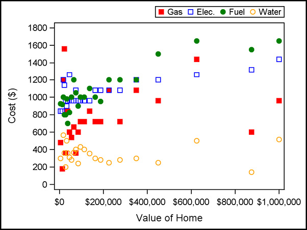
Plotting statements that create and display curve fits are also available as part of the SGPLOT procedure. Program 5.6.10 includes two polynomial regression curves (REG statement), a LOESS curve (LOESS statement), and a penalized B-spline (PBSPLINE statement). The statistical details of these curve fits, and others available in PROC SGPLOT, are beyond the scope of this book. However, the SAS Documentation contains further information about each of these methods and references other statistical publications.

Program 5.6.10: Fitting Curves for Utility Costs Versus Home Values

proc sgplot data= work.medians;

reg y=gas_median x=homevalue / degree=1 legendlabel=’Gas’

lineattrs=(color=red) markerattrs=(color=red symbol=squarefilled);

reg y=electric_median x=homevalue / degree=5 legendlabel=’Elec.’

lineattrs=(color=blue) markerattrs=(color=blue symbol=square);

loess y=fuel_median x=homevalue / legendlabel=’Fuel’

lineattrs=(color=green) markerattrs=(color=green symbol=circlefilled);

pbspline y=water_median x=homevalue / legendlabel=’Water’

lineattrs=(color=orange) markerattrs=(color=orange symbol=circle);

yaxis label=’Cost ($)’ values=(0 to 1600 by 200);

xaxis label=’Value of Home’ valuesformat=dollar12.;

keylegend / position=topright;

run;

 Like the SCATTER statement, each of these curve-fitting statements requires an X= and Y= variable. The curve is fit taking the Y= variable as a function of the X= variable.

 The REG statement fits a curve that is polynomial in the X= variable to the Y= variable. Though the available degrees of the polynomial fit vary across different maintenance releases of SAS, typically degrees from 1 to 10 are available.

 No matter which type of curve is fit, the curve itself is referred to as a line. Its attributes are set with LINEATTRS= and include COLOR=, THICKNESS=, and PATTERN=. PATTERN= includes both names and numbers as valid values. See the SAS Documentation for a list of names and numbers associated with various patterns.

 The LOESS and PBSPLINE statements fit a “smooth” curve to the data values. Both statements include the DEGREE= and SMOOTH= options to control the smoothness; however, they work differently for the two methods. See the SAS Documentation for more information and options.

Output 5.6.10: Fitted Curves for Utility Costs Versus Home Values

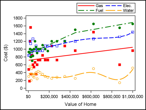
The previous examples used numeric variables exclusively for the X= and Y= variables, but these variables are not restricted to only the numeric type. Program 5.6.11 uses a character variable as one of the plotting variables and includes some options that are often helpful under that condition.

Program 5.6.11: Using a Categorical Variable with SCATTER

proc sgplot data=sashelp.cars;

scatter x=origin y=mpg_highway / jitter jitterwidth=0.8;

run;

 The variable Origin is not only categorical, it is stored as character—which is legal for use in either (or both) of the X= or Y= variable positions.

 When either variable is categorical, several data points can occupy the same position. The JITTER option moves observations slightly around the original position; balanced left-to-right when moving horizontally, or up-and-down when moving vertically.

 The amount of space available to jitter the points is controlled by the JITTERWIDTH= option. Much like the BARWIDTH= option introduced in Program 3.5.2, it sets the maximum area occupied by the jittered points as the proportion of available space.

Output 5.6.11: SCATTER Using a Categorical Variable

For these examples, plotting data for each of the utilities on the same graph requires multiple plotting statements which are subsequently overlaid. Section 5.7 shows a way to restructure the utility data and revisits these types of plots using the GROUP= option to also produce figures with distinct markers and/or curves for each utility type.

5.7 Restructuring Data with the TRANSPOSE Procedure

In the previous section, data for utility costs included one variable for each of four utilities. Under certain circumstances, it is advantageous (or even required) to restructure the data with one variable for the type of utility and another for its cost. This section shows how to perform this type of restructuring using the TRANSPOSE procedure and revisits some of the examples from Section 5.6 using this new data structure.

5.7.1 The TRANSPOSE Procedure

As a simple, preliminary example, Program 5.7.1 uses PROC TRANSPOSE with only a DATA= and OUT= option on a simplified data set.

Program 5.7.1: Transposing a Data Set

proc print data=sashelp.cars(keep=make model msrp mpg: obs=6) noobs;

run;

proc transpose data=sashelp.cars(keep=make model msrp mpg: obs=6)

out= work.carsTr;

run;

proc print data= work.carsTr noobs;

run;

 To make results easier to display, the Cars data is limited to a subset of the variables and observations available.

 Technically, OUT= is optional; however, PROC TRANSPOSE must produce a new data set to store the transposed data. If no name is supplied with the OUT= option, then SAS names the resulting data set automatically. It is considered a good programming practice to always explicitly name these output data sets.

Output 5.7.1 shows both the original data subset and its transpose. First, note that the make and model data do not appear in the transposed data set—only the numeric variables are transposed by default. However, a VAR statement is available to choose the variable values to be transposed, and character variables are only transposed when they are listed in it. Care should be taken with this as a record often contains a combination of character and numeric variables, but its transpose is to a single column. A column cannot contain both character and numeric types, so all values are converted to character.

Output 5.7.1: Transposing a Data Set

Make	Model	MSRP	MPG_City	MPG_Highway
Acura	MDX	$36,945	17	23
Acura	RSX Type S 2dr	$23,820	24	31
Acura	TSX 4dr	$26,990	22	29
Acura	TL 4dr	$33,195	20	28
Acura	3.5 RL 4dr	$43,755	18	24
Acura	3.5 RL w/Navigation 4dr	$46,100	18	24

_NAME_	_LABEL_	COL1	COL2	COL3	COL4	COL5	COL6
MSRP		36945	23820	26990	33195	43755	46100
MPG_City	MPG (City)	17	24	22	20	18	18
MPG_Highway	MPG (Highway)	23	31	29	28	24	24

Default behavior also includes naming the transposed variables with the prefix “col” and a numerical suffix and including a variable (_NAME_ by default) with values corresponding to the original variable names. In most cases a full transpose of rows and columns is not the objective; instead, like the example stated at the outset of this section, BY-group processing is exploited to transpose smaller structures throughout the data set. Program 5.7.2 turns each record from the utility cost data into four records, maintaining the Serial variable and replacing the four utility variables with one for utility type and another for the cost.

Program 5.7.2: Transposing Portions of Records Using BY-Group Processing

proc transpose data= work.ipums2005Utility out= work.Utility2;

by serial;

var electric--fuel;

run;

proc print data= work.Utility2(obs=8) noobs;

run;

 The requested transpose is now applied to each level of Serial. Since Serial is unique to each record, the transpose is applied on each record.

 The values of the four utility variables are transposed into three variables and four records. By default, the values of the transposed variables are assigned to the variable Col1 and the original variable names are assigned to the _NAME_ variable. The BY-group variable, Serial, is also preserved in the transposed data set.

 A subset of the transposed data is displayed in Output 5.7.2 to show the new structure.

Output 5.7.2: Transposing Portions of Records Using BY-Group Processing

serial	_NAME_	COL1
2	electric	$1,800
2	gas	$9,993
2	water	$700
2	fuel	$1,300
3	electric	$1,320
3	gas	$2,040
3	water	$120
3	fuel	$9,993

Options are given to set names for the transposed variables, though the RENAME= option is also available. Program 5.7.3 illustrates some strategies.

Program 5.7.3: Transposing Portions of Records Using BY-Group Processing

proc transpose data= work.ipums2005Utility name= work.Utility

prefix=Cost out= work.Utility2;

by serial;

var electric--fuel;

run;

proc transpose data= work.ipums2005Utility

out= work.Utility3(rename=(col1=Cost _name_=Utility));

by serial;

var electric--fuel;

run;

 The NAME= option replaces the default name of _NAME_ for the column containing the original variable name with the value specified.

 The PREFIX= option replaces the default prefix of COL for the names of the transposed variables. Whole number values are applied to each column resulting from the transpose. A SUFFIX= option is also available, with its value added to the end of the variable name following the column number.

 The RENAME= data set option can be applied to the output data set to directly set names of any columns, including those that result from the transpose operation.

If structure of the given data set is like that of Utility3 (four utility records on each value of Serial) and a structure like that of Ipums2005Utility (one record with four variables for each value of Serial) is desired, PROC TRANSPOSE can also perform this operation. Program 5.7.4 takes Utility3 as the input data set and returns it to the structure of the original Ipums2005Utility data.

Program 5.7.4: Transposing Multiple Records into a Set of Variables

proc transpose data= work.Utility3 out= work.Revert;

by serial;

var Cost;

run;

proc print data= work.Revert(obs=5) noobs;

run;

Output 5.7.4: Transposing Multiple Records into a Set of Variables

serial	_NAME_	COL1	COL2	COL3	COL4
2	Cost	$1,800	$9,993	$700	$1,300
3	Cost	$1,320	$2,040	$120	$9,993
4	Cost	$1,440	$120	$9,997	$9,993
5	Cost	$9,997	$9,993	$9,997	$9,993
6	Cost	$1,320	$600	$240	$9,993

Using BY-group processing results in the four records on the variable cost within each BY group for Serial being transformed into four variables on a single record for each unique Serial value. Here the _NAME_ variable is uniformly set to “Cost” and may not be particularly useful. The new variables containing utility costs have the default form of COL#, with # corresponding to the row order in the BY group.

A more useful set of variable names can be set using the RENAME= data set option; however, the TRANSPOSE procedure allows for another method via its ID statement. The ID statement uses the value of the selected variable as the name of the new variable, modifying those values to legal variable names if they do not satisfy proper naming conventions. (This modification produces variable names using the same process as PROC IMPORT, as shown in Program 3.8.1.) Program 5.7.5 uses the ID statement to select the values of the Utility variable as names for transposed cost values.

Program 5.7.5: Transposing Multiple Records into a Set of Variables

proc transpose data= work.Utility3 out= work.Revert2(drop=_name_);

by serial;

id Utility;

var Cost;

run;

proc print data= work.Revert2(obs=5) noobs;

run;

Output 5.7.5: Transposing Multiple Records into a Set of Variables

serial	electric	gas	water	fuel
2	$1,800	$9,993	$700	$1,300
3	$1,320	$2,040	$120	$9,993
4	$1,440	$120	$9,997	$9,993
5	$9,997	$9,993	$9,997	$9,993
6	$1,320	$600	$240	$9,993

If the ID statement uses more than one variable, their values are concatenated to form the variable name. The formation of these variable names also respects the PREFIX= and SUFFIX= options. Any records with missing values for the ID variable(s) are not included in the transpose. It is important to ensure that the ID variables are unique within each BY group and that the values align across BY groups—unintended or unexpected differences in spelling, casing, or spacing in text values can create unwanted results. For example, if Utility values for electricity are given the value Electric in some records and Electricity in others, two separate variables using these values as names are created in the transposed data, resulting in a misalignment. See Section 3.9 for data diagnostics and cleaning methods that are applicable in situations like these.

5.7.2 Revisiting Section 5.6 Examples Using Transposed Data

In Section 5.6.1, the utility cost data was originally read with a structure having each of the four utility costs in separate columns for each record corresponding to a unique value of Serial. In section 5.7.1, the TRANSPOSE procedure was used to restructure the data into four records for each unique value of Serial, having one variable for utility type and another for its corresponding cost. Each data structure has its advantages, and for certain operations or analyses only one of the two works. However, it is often true that either structure can be used to achieve the same result using slightly different syntax. This section revisits some of the examples of Section 5.6 using the transposed data, Utility3, created as part of Program 5.7.3.

Program 5.7.6 uses the transposed utility data (Utility3) to revisit the objectives of Programs 5.6.3 through 5.6.5, merging the utility and Ipums2005Basic data together and producing correlations between utility costs and other variables.

Program 5.7.6: Building Correlations Between Utility Costs and Other Variables from Transposed Data

data work.ipums2005cost2;

merge BookData.ipums2005basic work.Utility3;

by serial;

utility=propcase(utility);

label utility=’Utility’;

run;

proc sort data= work.ipums2005cost2;

by utility;

run;

proc corr data= work.ipums2005cost2;

by utility;

var cost;

with mortgagePayment hhincome homevalue;

where homevalue ne 9999999 and mortgageStatus contains ‘Yes’ and cost lt 9000;

ods select PearsonCorr;

run;

 The fundamental syntax of the merge does not change from Program 5.6.3, only the data set names are updated, as the matching still occurs on the Serial variable. However, it should be noted that this is now a one-to-many match rather than the one-to-one in Program 5.6.3.

 The values of the Utility variable are the original variable names chosen in the DATA step in Program 5.6.3 that read the Utility Cost 2005.txt file. To improve the display of these for later use, they are converted to proper case via the PROPCASE function.

 The CORR procedure does not allow for a CLASS statement; therefore, separating the analysis across utility types requires BY-group processing. Since the original merge has both data sets sorted on Serial, a subsequent sort on Utility is required prior to invoking PROC CORR.

 All the utility costs are now contained in the Cost variable, and the desired conditioning is achieved on this variable only—no resetting values to missing, as in Program 5.6.5, is required. However, a more defensive programming strategy of setting the values to missing is advised.

Output 5.7.6: Correlations Using Transposed Data (Partial Output)

Utility=Electric

Pearson Correlation Coefficients, N = 552600 Prob > \|r\| under H0: Rho=0
	Cost
MortgagePayment First mortgage monthly payment	0.22431 <.0001
HHINCOME Total household income	0.22240 <.0001
HomeValue House value	0.18481 <.0001

Utility=Fuel

Pearson Correlation Coefficients, N = 92646 Prob > \|r\| under H0: Rho=0
	Cost
MortgagePayment First mortgage monthly payment	0.18342 <.0001
HHINCOME Total household income	0.16220 <.0001
HomeValue House value	0.20998 <.0001

Program 5.7.7 also uses the transposed utility data (Utility3) to revisit the objectives of Programs 5.6.9, using the GROUP= option in the SCATTER statement to make a graph like that of Output 5.6.9.

Program 5.7.7: Making Scatterplots Based on Transposed Utility Data

ods listing close;

proc means data= work.ipums2005cost2 median;

var cost;

class homevalue utility;

where state eq ‘Vermont’ and homevalue ne 9999999 and cost lt 9000;

ods output summary= work.medians2;

run;

ods listing;

proc sgplot data= work.medians2;

scatter y=cost_median x=homevalue / group=utility;

yaxis label=’Cost ($)’ values=(0 to 1600 by 200);

xaxis label=’Value of Home’ valuesformat=dollar12.;

keylegend / position=topright;

run;

 Adding Utility as a class variable produces the summary statistic for each of the four utility types, ensuring the Utility variable is available in the output data set.

 Again, the single analysis variable is Cost and it can be effectively conditioned for all records on all utility types without special intervention.

 The GROUP= option distinguishes the observations on the plot across the four utility types. Looking at the legend in Output 5.7.7, note the value of using the PROPCASE function on the original variable names.

 The XAXIS, YAXIS, and KEYLEGEND statements are unaltered from those used in Program 5.6.9.

Output 5.7.7: Scatterplots Based on Transposed Utility Data

Since Program 5.7.7 does not include any options to modify the scatterplot markers, the colors and symbols used for them are the same as those shown in Output 5.6.8. When using the GROUP= option, control of markers and lines is handled somewhat differently. Program 5.7.8 uses the MARKERATTRS= option to make a limited modification to the markers.

Program 5.7.8: Setting Attributes for Markers in Grouped Scatter Plots

proc sgplot data= work.medians2;

scatter y=cost_median x=homevalue / group=utility markerattrs=(symbol=square);

yaxis label=’Cost ($)’ values=(0 to 1600 by 200);

xaxis label=’Value of Home’ valuesformat=dollar12.;

keylegend / position=topright;

run;

Output 5.7.8: Setting Attributes for Markers in Grouped Scatter Plots

The SYMBOL= attribute makes the symbol for each group a square, leaving the color cycle as the only distinguishing feature among the levels of Utility. Setting both COLOR= and SYMBOL= attributes in the MARKERATTRS= option makes the groups indistinguishable. Since the ability to control the full set of colors and symbols (and line types) is desirable for these plots as well, Program 5.7.9 shows one method to take control of these sets.

Program 5.7.9: Using the STYLEATTRS Statement to Set Attributes in Grouped Plots

proc sgplot data= work.medians2;

styleattrs datacontrastcolors=(red blue green orange)

datasymbols=(circle square triangle diamond)

datalinepatterns=(solid);

pbspline y=cost_median x=homevalue / group=utility;

yaxis label=’Cost ($)’ values=(0 to 1600 by 200);

xaxis label=’Value of Home’ valuesformat=dollar12.;

keylegend / position=topright;

run;

 The STYLEATTRS statement allows for setting style attributes broadly, across all plotting statements included in the PROC SGPLOT call.

 The DATACONTRASTCOLORS= option specifies a list of colors to be applied to markers and lines. This modifies the list of colors SAS cycles through as it moves through levels of a GROUP= variable or as it moves through different plotting statements to be overlaid. DATACOLORS= is also available to modify fill colors.

 The DATASYMBOLS= option modifies the list of marker symbol shapes SAS cycles through.

 The DATALINEPATTERNS= option sets the list of line styles SAS cycles through. For any of these lists, it is important to ensure the number of elements of the list is sufficient to properly distinguish the different categories on the graph. In Output 5.7.9, the four levels of Utility each have different colors for lines and markers along with different marker shapes; however, each uses the same line type.

Output 5.7.9: Using the STYLEATTRS Statement to Set Attributes in Grouped Plots

As an exercise, and to see that this behavior is not limited to the GROUP= option, remove the MARKERATTS= and LINEATTRS= option from each of the plotting statements in Program 5.6.10, add the STYLEATTRS statement used in Program 5.7.9, and submit the new version—the cycling of colors, symbols, line styles matches that of Output 5.7.9. However, note that Output 5.6.10 cannot be reproduced using a GROUP= option on the transposed data—Program 5.6.10 overlays plots of different types, while GROUP= splits across levels of the specified variable in a single plot type.

5.8 Wrap-Up Activity

Use the lessons and examples contained in this and previous chapters to complete the activity shown in Section 5.2.

Data

Various data sets are available for use to complete the activity. This data expands on the data used in the Wrap-Up Activity for Chapter 4, bringing in utility data for 2005 used in the in-chapter examples, plus similar data for 2010 and 2015. Completing this activity requires the following files:

Ipums2005Basic.sas7bdat
Ipums2010Basic.sas7bdat
Ipums2015Basic.sas7bdat
Utility Cost 2005.txt
Utility Costs 2010.csv
2015 Utility Cost.dat

Scenario

Use the skills mastered so far, including those from previous chapters, to assemble the listed files into a single data set and create the analyses shown in Section 5.2. To get the maximum benefit from this activity, build the graphs shown in 5.2.2 and 5.2.3 from the data assembled in its original form and also from appropriately transposed versions of that data.

5.9 Chapter Notes

1. Special Missing Numeric Values. Program 5.3.5 demonstrates using conditional logic to assign values to missing using the standard numeric missing value—a single period. However, SAS provides 27 distinct special missing values for a numeric variable in addition to the standard missing value. The special missing values are denoted by a period followed by either an underscore or a letter (._, .A, .B, …, .Z). While a lowercase letter is valid during assignment, SAS displays these values using capital letters. Because the values are distinct, SAS assigns them different sort priorities with ._ being the smallest special missing value, the standard missing value is the second smallest, then .A through .Z with .Z being the largest missing value. The sort order is important when using numeric missing values in ranges as using the standard missing value as the lower bound, such as in a format, would exclude missing values encoded with ._, but would include all other missing values. To exclude all missing values, a range must use .Z as the excluded lower bound of the range.

Special missing values are useful when a variable, such as the utility cost variables in the IPUMS CPS data sets, have missing values for multiple reasons. Program 5.9.1 demonstrates assigning two special missing values, .A and .B, based on the fact that in the IPUMS 2005 data a value of 9993 and 9997 had specific meanings. Outputs 5.9.1A and 5.9.1B show the results of displaying these special missing values with and without the application of a format.

Program 5.9.1: Assigning and Using Special Missing Values

data ipums2005UtilityB;

infile RawData(‘Utility Cost 2005.txt’) dlm=’09’x dsd firstobs=4;

input serial electric:comma. gas:comma. water:comma. fuel:comma.;

format electric gas water fuel dollar.;

if electric eq 9993 then electric=.A;

else if electric eq 9997 then electric=.B;

run;

proc freq data = ipums2005UtilityB;

table electric / missing;

where electric in (.A, .B);

run;

proc format;

value elecmiss .A = ‘No Charge or None Used’

.B = ‘Included in Rent or Condo Fee’

;

run;

proc freq data = ipums2005UtilityB;

table electric / missing;

where electric in (.A, .B);

format electric elecmiss.;

run;

Output 5.9.1A: Using Special Missing Values without Applying a Format

electric	Frequency	Percent	Cumulative Frequency	Cumulative Percent
A	9428	21.10	9428	21.10
B	35244	78.90	44672	100.00

Output 5.9.1B: Using Special Missing Values with a Format

electric	Frequency	Percent	Cumulative Frequency	Cumulative Percent
Included in Rent or Condo Fee	35244	78.90	35244	78.90
No Charge or None Used	9428	21.10	44672	100.00

1. Updating and Modifying. The DATA step offers two additional techniques for combining information from multiple SAS data sets: updating and modifying. These techniques are most similar to the horizontal techniques discussed in Section 5.3. The UPDATE statement, as the name implies, is useful for adding new information into an existing data set. It requires a BY statement to join records between a master data set and a transaction data set. Records with matching values of the key variables in both data sets are updated so that any new information from the transaction data set is copied into the master data set. UPDATE is very similar to MERGE, with the notable exception that MERGE overwrites nonmissing data with missing data unless conditional logic is present to prevent it from occurring. The UPDATE statement can have the same behavior, but its default is to not overwrite nonmissing values with missing data. The MODIFY statement offers some of the same functionality, but with an expanded set of options and risks. For more information about the MODIFY statement, see the SAS Documentation.

2. Semijoins and Antijoins. Semijoins are directional, just like left and right joins. The effect of a semijoin is to filter a table based on whether its records have matching key variable values in another table; however, no information from the second table is included in the resulting semijoin. For example, a left semijoin of two tables, A and B, returns all the rows in A that have matching key variable values in B. This is very similar to a left join, but a left semijoin only returns the columns from A, while a left join returns the columns of both A and B. An antijoin is the row-complement of a semijoin; a left antijoin of the tables A and B returns all the rows in A for which the key variables do not have a match in table B. Like left semijoins, a left antijoin of tables A and B does not include any columns from table B. While the examples here are for left semijoins and antijoins, right semijoins and antijoins work in an equivalent manner. In the DATA step, use the IN= data set options and conditional logic along with KEEP and DROP lists to produce semijoins or antijoins.

3. The DELETE Statement. In addition to providing the OUTPUT statement discussed in Section 5.5, SAS provides the closely related DELETE statement. Recall, using OUTPUT in a program forces the DATA step to immediately write the current PDV to the data set but continues executing any remaining statements in the DATA step. Conversely, using DELETE prevents the DATA step from writing the current PDV to the resulting DATA set and immediately returns control to the top of the DATA step, foregoing the execution of any remaining programming statements during the current iteration of the DATA step. As a result, the following two statements are equivalent.

IF expression;

IF NOT (expression) THEN DELETE;

Due to their ability to avoid complex operations on unwanted observations, the subsetting IF and DELETE statements are both important tools when computational efficiency is a priority.

5.10 Exercises

Concepts: Multiple Choice

1. If the SAS data set Mayflies exists in the work library, what output is produced by the following code?

proc corr data = Mayflies;

run;

a. None—it generates an error in the log.

b. None—it generates a warning in the log.

c. Correlations and associated statistics on all variables in the data set.

d. Correlations and associated statistics on all numeric variables in the data set.

2. If the SAS data set DataDivas exists in the work library, what result is produced by the following code?

proc transpose data = DataDivas;

run;

a. None—the OUT= option must be used to specify where to store the transposed results.

b. Transposes of all variables in the data set.

c. Transposes of all numeric variables in the data set.

d. Transposes of all character variables in the data set.

3. Assuming the SAS data set DataDivas exists in the work library, which of the following measures of association are produced by the following code?

proc freq data = DataDivas;

table Size*FileType / norow format = comma8.;

run;

a. None—the CORR option is required.

b. None—the MEASURES option is required.

c. Only Pearson correlations between Size and FileType.

d. Pearson and Spearman correlations between Size and FileType.

4. Consider the data set, Diagnosis, shown in the following table.

Diagnosis

Subject	Visit	DiagnosisCode
001	1	450
001	2	430
001	3	410
002	1	250
002	2	240
003	1	410
003	2	250
003	3	500
004	1	240

After running the following TRANSPOSE procedure, which of the answer choices below shows the resulting data set? (Assuming none of the variables have associated labels.)

proc transpose data = Diagnosis prefix = Dx

out = Rotated(drop = _NAME_);

by Subject;

id Visit;

var DiagnosisCode;

run;

Subject	Dx1	Dx2	Dx3
001	450	430	410
002	250	240	.
003	410	250	500
004	240	.	.

Subject	001	001	001	002	002	003	003	003	004
Visit	1	2	3	1	2	1	2	3	1
Diagnosis	450	430	410	250	240	410	250	500	240

Subject	Visit	Dx1	Dx2	Dx3
001	1	450	430	410
001	2	450	430	410
001	3	450	430	410
002	1	250	240	.
002	2	250	240	.
003	1	410	250	500
003	2	410	250	500
003	3	410	250	500
004	1	240	.	.

d. None of the above

5. Consider the data set, Height, shown in the following table.

Height

Height1	Height2	Height3
1	11	101
2	12	102
3	13	103
4	14	104
5	15	105

After running the following TRANSPOSE procedure, which of the answer choices below shows the resulting data set if none of the variables have associated labels?

proc transpose data = Height out = HeightRows;

var Height3 Height2 Height1;

run;

_NAME_	COL1	COL2	COL3	COL4	COL5
Height1	1	2	3	4	5
Height2	11	12	13	14	15
Height3	101	102	103	104	105

COL1	COL2	COL3	COL4	COL5
1	2	3	4	5
11	12	13	14	15
101	102	103	104	105

Height1	Height2	Height3	Height4	Height5
1	2	3	4	5
11	12	13	14	15
101	102	103	104	105

d. None of the above

6. Consider the Weight and Visit data sets shown below.

Weight (left) and Visit (right)

Subject	Visit	Weight	Subject	Visit	Date
1	1	101	1	1	18JAN2019
1	2	102	1	2	19JAN2019
2	1	103	1	3	20JAN2019
3	1	104	2	1	01FEB2019
3	2	105	2	2	03FEB2019

What type of join does the following DATA step carry out?

data combined;

merge weight visit;

by subject;

run;

a. One-to-one merge

b. One-to-one match-merge

c. One-to-many match-merge

d. Many-to-many match-merge

7. Using the data sets and code from the previous question, how many records appear in the data set Combined.

a. 0—no data set is produced due to an error

b. 5

c. 7

d. 10

8. The following DATA step is submitted.

data work.combined;

merge work.Employee work.Demog;

run;

A character variable named EmpID is contained in both the Work.Employee and Work.Demog data sets. The variable EmpID has a length of six in Work.Employee and a length of eight in Work.Demog. What is the length of the variable EmpID in the Work.Combined data set?

a. 6—because it is the first length from the two input data sets

b. 8—because it is the larger length from the two input data sets

c. 8—because it is the default length for character variables

d. 8—because it is the last length from the two input data sets

9. Selected components of the descriptor portions of the Employee and Demog data sets are shown below.

Data Set	Variable	Type	Length	Format	Label
Employee	EmpID	Char	6	$6.
	HireDate	Num	8	date9.	Date of Hire
	Salary	Num	8	dollar13.2	Current Salary
Demog	EmpID	Char	8	$6.	Employee ID
	HireDate	Num	8	mmddyy10.	Hire Date

If the following DATA step is submitted using the data sets described above, which of the answer choices below correctly identifies the format for HireDate?

data example;

merge employee demog;

by EmpID;

run;

a. DATE9.

b. MMDDYY10.

c. DATE10.

d. MMDDYY9.

10. Using the descriptor information and DATA step code from the previous question, which of the answer choices below correctly identifies the label for EmpID in the Example data set?

a. EmpID

b. Employee ID

c. None—there is no label for this variable in the Employee data set.

d. Employ

11. Consider the data set, OutputControl, shown below.

OutputControl

Y	Z
1	11
2	12
3	13
2	14
5	15
2	16

If the following program is submitted, how many observations are in each data set?

data A B;

set OutputControl;

if Y = 1 then output A;

else if Y = 2 then output B;

else output;

run;

a. A has 1 observation, B has 3 observations

b. A has 1 observation, B has 5 observations

c. A has 3 observations, B has 3 observations

d. A has 3 observations, B has 5 observations

12. Consider the data set, Quarks, shown below.

Quarks

Flavor	Sequence
Up	1
Down	2
Charm	3
Up	4
Strange	5
Charm	6

If the following program is submitted, how many observations are in each data set?

data Up Down Others;

set Quarks;

if Flavor = ‘Up’ then output Up;

else if Flavor = ‘Down’ then output Down;

run;

a. Up has 2 observations, Down has 1 observation, Others has 3 observations

b. Up has 2 observations, Down has 1 observation, Others has 0 observations

c. Up has 5 observations, Down has 4 observations, Others has 0 observations

d. Up has 5 observations, Down has 4 observations, Others has 3 observations

13. The Start data set is shown in the table below.

Start

Var1	Var2
A	3
B	5
C	8

How many records appear in each of the data sets created by the following DATA step?

data ID Count;

set start;

if var1 = ‘D’ then output ID;

run;

a. ID has 3 observations, Count has 3 observations

b. ID has 0 observations, Count has 3 observations

c. ID has 3 observations, Count has 0 observations

d. ID has 0 observations, Count has 0 observations

14. Consider the data sets Model and Retail shown in the following tables.

Model

Brand	ModelID
Sunny	SN-657-NK
Acre	TG-983-FP

Brand

Brand	Retail
Sunny	$400
Sunny	$350
Dull	$370
Dull	.

If the following DATA step is submitted, which of the answer choices shows the resulting data set?

data work.all;

merge work.model work.retail;

by descending brand;

run;

Brand	ModelID	Retail
Sunny	SN-657-NK	$400
Sunny	TG-983-FP	$350

Brand	ModelID	Retail
Sunny	SN-657-NK	$400
Sunny	SN-657-NK	$350
Dull		$370
Dull		.
Acre	TG-983-FP	.

Brand	ModelID	Retail
Sunny	SN-657-NK	$400
Sunny	TG-983-FP	$350
Dull		$370
Dull		.

Brand	ModelID	Retail
Sunny	SN-657-NK	$400
Sunny		$350
Dull		$370
Dull		.
Acre	TG-983-FP	.

Concepts: Short-Answer

1. Consider the different methods for combining three data sets—A, B, and C—in the DATA step. If the data sets contain a common variable named Sequence, and each data set is sorted by Sequence in ascending order, briefly describe the process SAS uses to join the records from the three input data sets in the following scenarios:

b. Each data set appears in its own SET statement.

c. All data sets appear in the same MERGE statement without a BY statement.

d. All data sets appear in the same MERGE statement, and Sequence is used as the only BY variable.

2. In PROC SORT, the OUT= option prevents SAS from replacing the original data set with the new, sorted, data set. In contrast, the TRANSPOSE procedure creates a new data set even if the OUT= is absent. Why is the default in PROC TRANSPOSE to not overwrite the original data?

3. In PROC TRANSPOSE, the PREFIX= and SUFFIX= options allow for customization of the variable names for any newly-created columns that result from rows in the input data set. Given the existence of these options, justify the existence of the ID statement by explaining how it differs from the PREFIX= and SUFFIX= options.

4. When investigating the association between two numeric variables, why is it typically not useful to apply a user-defined format (or even certain formats provided by SAS) to either of those numeric variables in PROC CORR when it is often quite useful to do so in PROC FREQ?

5. Consider the three data sets shown below: Contacts, Sales, and FilingDate.

Contracts (left), Sales (middle), and FilingDate (right)

CustomerID	Contact	CustomerID	QTR	Sales	CustomerID	Date
1	Fulanah AlFulaniyyah	1	1	18000	1	01JAN2019
2	John Doe	1	2	23000	1	01APR2019
3	Tran Thi B	1	3	15000	1	01JUL2019
4	Yossi Cohen	1	4	35000	1	01OCT2019
		2	1	22000	3	01JAN2017
		2	2	10000	4	01JAN2018
		2	3	8000	4	01APR2018
		2	4	40000	4	05APR2018
		4	1	20000	4	01JUL2018
		4	2	25000	4	09OCT2018
		4	3	22000	5	14APR2019
		4	4	24000	5	31DEC2019
		5	1	90000
		5	2	120000
		5	3	85000
		5	4	140000

e. Without executing the program below in a SAS session, write out the values of the user-defined variables in the PDV for iterations 2, 6, 9, and 10 of the following DATA step.

data Accounting;

merge contacts sales filingdate;

by customerID;

run;

f. If the variable Qtr is added to the FilingDate data set, is it possible to update the program in (a) so that it produces a one-to-many match-merge of the three provided data sets? Assume Qtr only takes on the values 1, 2, 3, or 4 and is not missing for any record.

14. Consider two data sets, A and B, that are connected through a single key variable, X. Describe the relationship between: the left antijoin of A with B, the right antijoin of A with B, the inner join of A with B, and the full outer join of A with B.

15. Explain why no observations appear in either of the created data sets when using the following DATA step.

data CompanyA CompanyB;

set employee(where = (Age < 25));

if Age eq 30 then output;

run;

Programming Basics

1. The following graph was generated using three variables from the Sashelp.Stocks data set: Stock (the name of the stock), High (the maximum value at which the stock was traded on a given date), and Date (the date on which the value of High was recorded).

image shown here

a. Use the Sashelp.Stocks data set to generate the graph shown above.

b. After submitting the following code, use the StockTr data set to create the graph shown above.

proc sort data=sashelp.stocks out=stockSort;

by date;

run;

proc transpose data=stockSort out=stockTr;

var high;

by date;

id stock;

run;

c. Compare the two SGPLOT procedures from part (a) and part (b). Which of the two techniques would scale up more easily to scenarios that needed to graph 500 different stocks instead of three?

2. Use the following code to create a subset of the Sashelp.Prdsale data set and exchange some row and column information from the subset.

proc sort data = sashelp.prdsale out = prdSubset(drop = year);

by country region division prodtype product quarter;

where year eq 1993;

run;

proc transpose data = PrdSubset out = salesWide prefix = month;

by country region division prodtype product quarter;

var actual predict;

run;

a. Write a program that reverses the transposition and recovers the PrdSubset data set.

b. Validate that the PrdSubset data generated by reversing the transposition matches the PrdSubset data set generated by the SORT procedure above.

3. Write a program that uses the Sashelp.Baseball data set and produces only the following output.

Pearson Correlation Coefficients, N = 322 Prob > \|r\| under H0: Rho=0
	nHome	nRuns	nRBI
nHits Hits in 1986	0.54165 <.0001	0.91167 <.0001	0.79311 <.0001
nBB Walks in 1986	0.46835 <.0001	0.71288 <.0001	0.59070 <.0001

4. Use the BookData.Visit and BookData.PayStatus data sets to write a program that does the following in a single DATA step.

◦ Joins the data sets by PatientID

◦ Creates three data sets: AllRecords, Match, and Mismatch

◦ Ensure every record goes into the AllRecords data set; only records that come from both data sets go into the Match data set; records that only come from one data set go into the Mismatch data set

◦ Writes the PDV to the log any time a mismatched observation is written to the Mismatch data set

5. Use the Sashelp.Citimon and Sashelp.Citiday data sets to answer the following questions.

a. What variables are available for use as key variables during a match-merge? Are the values useful for carrying out a match-merge?

b. Write a DATA step that carries out a one-to-many match-merge so that the monthly indicators from Sashelp.Citimon are joined with each record from the same month in Sashelp.Citiday. Ensure that only records from Sashelp.Citiday remain in the final data set.

6. Program 5.3.6 created several difference and ratio variables. In that program, operations on missing values result in unnecessary—and in some industries, unallowed—notes in the log. Similarly, division by zero results in the DATA step setting _ERROR_ to 1 and writing the associated messages to the log. Write a DATA step that produces equivalent results but without generating any notes, warnings, or errors as a result of operations on missing values or division by zero.

Case Studies

For additional practice, multiple case studies are available in addition to the IPUMS CPS case study used in the chapters. See Section 8.5 to apply the skills from this chapter to the Clinical Trials Case Study. For additional case studies, including extensions to the IPUMS CPS case study, see the author pages.

..................Content has been hidden....................

You can't read the all page of ebook, please click here login for view all page.

Table of Contents for Chapter 5: Joining Data Sets on Common Values and Measuring Association

Create new playlist

Sign In

Sign Up

Table of Contents for
Chapter 5: Joining Data Sets on Common Values and Measuring Association