
Chapter 2
Symmetry, Stability and Scalability
People today see not the moon the ancients saw, and yet this moon shone once upon the ancients.
—Li Bai (701–762), ‘Inquiring of the moon, with wine in hand'
This chapter introduces general models of distributed control systems based on graph theory and linear system theory. The symmetry property of distributed control systems in the frequency domain is defined and investigated. Classic results of the frequency-domain test of the stability of multivariable feedback control systems are reviewed with the emphasis on their extension to the semi-stability and the scalability for distributed control systems.
2.1 System Model
2.1.1 Graph-Based Model of Distributed Control Systems
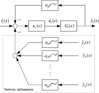
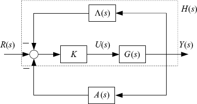
Consider a distributed control system with n subsystems, each of which is also called an agent in this book. Let the model of the dynamics of the ith agent be given by the following state-space model
where ![]() ,
, ![]() and
and ![]() denote the state, input and output, respectively, of the ith agent, Ti is the input delay. Note that in distributed control systems input delays are usually caused by the processing time for the packets arriving at each agent and/or the communication time between actuators and controllers.
denote the state, input and output, respectively, of the ith agent, Ti is the input delay. Note that in distributed control systems input delays are usually caused by the processing time for the packets arriving at each agent and/or the communication time between actuators and controllers.
The agents are interconnected according a fixed topology which can be described by a digraph ![]() of order n. Denote by Ni the set of neighbors of agent i. By (1.9), the aggregated measurement of agent i is based on the information from its neighbors and itself:
of order n. Denote by Ni the set of neighbors of agent i. By (1.9), the aggregated measurement of agent i is based on the information from its neighbors and itself:
where τij is the communication delay from agent j to agent i which mainly consists of propagation delay and queueing delay, τii is called self-delay which is often introduced to match the communication delays, aij is the weight for the output channel from agent j to agent i and aii is the weight for the self-loop of agent i. To incorporate the aggregated measurement (1.9) and the relative measurement (1.10) in a unified form, throughout this chapter, we assume that aij in (2.2) can be either positive or negative.
Suppose that agent i is manipulated by the following local controller
where ![]() is the state of the local controller for agent i,
is the state of the local controller for agent i, ![]() are parameters of the controller and ri(t) is some reference signal for agent i.
are parameters of the controller and ri(t) is some reference signal for agent i.
Denote by Gi(s) the transfer function of agent i, i.e.,
(2.4) ![]()
and by κi(s) the transfer function of the ith controller, i.e.,
(2.5) ![]()
The feedback control system for agent i is shown in Figure 2.1. Let ![]() and
and ![]() be the Laplace transformation of the output and input, respectively, of the i-agent. Denote
be the Laplace transformation of the output and input, respectively, of the i-agent. Denote
(2.6) ![]()
(2.7) ![]()
(2.8) ![]()
(2.9) ![]()
(2.10) ![]()
and
A(s) and ![]() can be considered as the weighted adjacency matrix and generalized weighted adjacency matrix, respectively, of topology digraph G. As a matter of fact, in our model the matrix
can be considered as the weighted adjacency matrix and generalized weighted adjacency matrix, respectively, of topology digraph G. As a matter of fact, in our model the matrix ![]() can be further extended to the following form
can be further extended to the following form
(2.13) ![]()
where the transfer function ![]() describes the possible dynamics of the communication channel from agent j to agent i.
describes the possible dynamics of the communication channel from agent j to agent i.
Figure 2.1 Feedback control system of agent i.
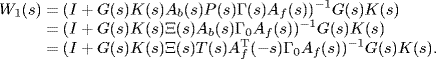
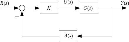
With notations introduced above, the closed-loop system composed of (2.1), (2.2) and (2.3) can be sketched in Figure 2.2. The transfer function matrix from R(s) to Y(s) is given by
Figure 2.2 Diagram of distributed control system.
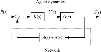
The system shown in Figure 2.2 is an interconnection of two parts. The first part G(s)K(s) is a diagonal matrix, which represents the agent dynamics. The second part A(s) + Λ(s) can be considered as a generalized complex adjacency matrix of the topology graph of the network; it reflects both the topology and the channel dynamics of the network used by the multi-agent system.
Definition 2.1 The dynamics of the agents in the distributed control system shown in Figure 2.1 are said to be homogeneous if κi(s)Gi(s) = κj(s)Gj(s) for all ![]() ; the network through which the agents are interconnected is said to be homogeneous if τij = τ0 and αij(s) = α0(s),
; the network through which the agents are interconnected is said to be homogeneous if τij = τ0 and αij(s) = α0(s), ![]() , where
, where ![]() and
and ![]() . The distributed control system is said to be homogeneous if all the agents and the network are all homogeneous. Otherwise, the agents (network) are said to be heterogeneous if they are not homogeneous. The system is said to be heterogeneous if it contains heterogeneous agents or heterogeneous network.
. The distributed control system is said to be homogeneous if all the agents and the network are all homogeneous. Otherwise, the agents (network) are said to be heterogeneous if they are not homogeneous. The system is said to be heterogeneous if it contains heterogeneous agents or heterogeneous network.
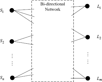
2.1.2 Bipartite Distributed Control Systems
There are many distributed control systems in which information exchanges are conducted through forward and backward channels. The interconnection of agents in such systems can be described by the weighted bipartite digraph shown in Figure 2.3. We call these systems bipartite systems. Denote by (S, L) and A the vertex bipartition and the weighted adjacency matrix of the graph, respectively, where
(2.15) ![]()
(2.16) ![]()
Let the agents associated with vertex class S be described by transfer functions Gi(s), ![]() ; and the agents associated with L be described by transfer functions Pj(s),
; and the agents associated with L be described by transfer functions Pj(s), ![]() . Agent i in S receives output information from its neighbors in L, and agent j in L receives output information from its neighbors in S, i.e.,
. Agent i in S receives output information from its neighbors in L, and agent j in L receives output information from its neighbors in S, i.e.,
(2.18) ![]()
(2.19) ![]()
Figure 2.3 Bipartite graph for distributed control systems.
where ![]() ,
, ![]() are the communication delay and the weight of the backward channel from agent l in L to agent i in S, respectively;
are the communication delay and the weight of the backward channel from agent l in L to agent i in S, respectively; ![]() ,
, ![]() are the communication delay and the weight of the forward channel from agent i in S to agent l in L. Considering (2.17), the following relationship should hold
are the communication delay and the weight of the forward channel from agent i in S to agent l in L. Considering (2.17), the following relationship should hold
Agent i in S is manipulated by dynamic controller κi(s), i = 1, ![]() , n, and agent l in L is manipulated by dynamic controller γl(s), l
, n, and agent l in L is manipulated by dynamic controller γl(s), l ![]() 1,
1, ![]() , m. Denote by
, m. Denote by
![]()
and
![]()
the reference input vector and output vector of all the agents in S, respectively; by
![]()
and
![]()
the reference input vector and output vector of all the agents in L, respectively. Then, the bipartite system with forward and backward channels can be shown by Figure 2.4, where
Figure 2.4 Bipartite distributed control system.
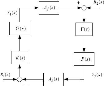
The transfer function matrix from R1(s) to Y1(s) is given by
(2.21) ![]()
and the transfer function matrix from R2(s) to Y2(s) is given by
(2.22) ![]()
Denote ![]() and
and ![]() . Then, the open-loop transfer function of W1(s) or W2(s) has the same structure as that of W(s) given by (2.14), i.e., it consists of a diagonal matrix corresponding to the agents' dynamics and a square matrix corresponding to the topology graph. This suggests that it is possible to deal with the stability problem of two kinds of distributed control systems in a unified framework.
. Then, the open-loop transfer function of W1(s) or W2(s) has the same structure as that of W(s) given by (2.14), i.e., it consists of a diagonal matrix corresponding to the agents' dynamics and a square matrix corresponding to the topology graph. This suggests that it is possible to deal with the stability problem of two kinds of distributed control systems in a unified framework.
2.2 Symmetry in the Frequency Domain
2.2.1 Symmetric Systems
In practice, many multi-agent systems are based on networks with undirected topology graph. In this case, if there is no delay and all the channels have constant dynamics, i.e., τij = 0 αij(s) = 1, ![]() , then the system shown in Figure 2.2 is said to be symmetric because the adjacency matrix of the topology graph is symmetric. Can such a conception of symmetry be extended to the case when there are non-zero delays or non-constant dynamics in network channels? In this book, we define the symmetry of networked-based distributed control systems as follows.
, then the system shown in Figure 2.2 is said to be symmetric because the adjacency matrix of the topology graph is symmetric. Can such a conception of symmetry be extended to the case when there are non-zero delays or non-constant dynamics in network channels? In this book, we define the symmetry of networked-based distributed control systems as follows.
Definition 2.2 Let the open-loop transfer function of a distributed control system be given by ![]() , where
, where ![]() is a diagonal matrix and
is a diagonal matrix and ![]() is a square matrix. The system is said to be symmetric if
is a square matrix. The system is said to be symmetric if ![]() can be decomposed as
can be decomposed as
(2.23) ![]()
where Θ(s) is a diagonal matrix and ![]() satisfies the following condition:
satisfies the following condition:
A starting point for this definition is that a complex generalized adjacency matrix of an undirected graph should be a Hermitian matrix as we defined in Chapter 1. Indeed, letting s = jω, then from (2.24) we have ![]() . So, if we absorb the diagonal matrix Θ(s) in the agents' dynamics which also form a diagonal matrix, then
. So, if we absorb the diagonal matrix Θ(s) in the agents' dynamics which also form a diagonal matrix, then ![]() can be regarded as a generalized adjacency matrix of the undirected topology graph in the frequency domain.
can be regarded as a generalized adjacency matrix of the undirected topology graph in the frequency domain.
Example 2.3 Symmetry in the frequency domain.
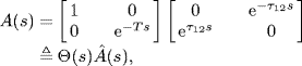
Consider the simplest undirected graph of two nodes, shown by Figure 2.5. Suppose the communication delays from node 1 to node 2 and from node 2 to node 1 are τ21 > 0 and τ12 > 0, respectively. It is natural to set e−τ12s and e−τ21s as the weights in the Laplace domain. But, the matrix
![]()
Figure 2.5 Symmetry in the frequency domain.
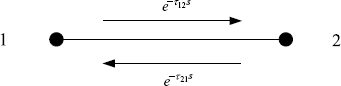
does not satisfy conjugate symmetry even in the case τ12 = τ21 = τ. In the frequency domain, A(jω) is not a Hermitian matrix, either. Now, let us scale the matrix A(s) by multiplying
where
(2.25) ![]()
which is called the round-trip time between node 1 and node 2. Then, we find that
where ![]() is a diagonal matrix,
is a diagonal matrix, ![]() satisfies
satisfies ![]() , and hence,
, and hence, ![]() is a Hermitian matrix. So, by Definition 2.2, the system based on the graph shown in Figure 2.5 is symmetric in the frequency domain even if τ12 ≠ τ21.
is a Hermitian matrix. So, by Definition 2.2, the system based on the graph shown in Figure 2.5 is symmetric in the frequency domain even if τ12 ≠ τ21.
Absorbing Θ(s) into the diagonal transfer function matrix of the agents implies that the agent associated with node 2 obtains an additional time delay T. So, this example shows that sometimes the frequency-domain symmetry of a communication topology can be achieved by introducing a lag in the time domain for agents!
Now, let us consider the general distributed control system composed of (2.1), (2.2) and (2.3) or equivalently the system shown in Figure 2.1. Assume the interconnection topology graph of the system is undirected. Then, to match the symmetry requirement of Definition 2.2, there should exist ![]() , such that
, such that
It is said that the system has symmetric communication delays if the requirement (2.26) is satisfied. Note that the symmetric communication delay does not imply τij = τji.
2.2.2 Symmetry of Bipartite Systems
Before we study the symmetry property of bipartite systems with forward and backward channels, let us introduce the notion of semi-homogeneousness as follows.
Definition 2.4 Consider a bipartite system which is based on the bipartite graph G(S ⊕ L). It is said to be semi-homogeneous by vertex L if for each agent i in S, the following conditions are satisfied:
Similarly, one can also define the semi-homogeneousness of the system by vertex class S.
Remark. Obviously, if all the agents in vertex class L have homogeneous dynamics, (2.27) holds.
The next theorem shows that the technique used in Example 2.3 can be applied to general semi-homogeneous bipartite systems.
Theorem 2.5 If the system based on the bipartite graph G(S ⊕ L) is semi-homogeneous by L or by S, then it is symmetric in the frequency domain.
Proof. We just consider the case that the system is semi-homogeneous by L. The proof for the other case is the same.
Denote Γ0 = diag{γ1, ![]() , γm} and Ξ(s) = diag{α1(s),
, γm} and Ξ(s) = diag{α1(s), ![]() , αn(s)}. Then, under assumption (2.27) we have
, αn(s)}. Then, under assumption (2.27) we have
![]()
Denote T(s) = diag{e−T1s, ![]() , e−Tns}. Then, by using (2.20) and (2.28), one can see that
, e−Tns}. Then, by using (2.20) and (2.28), one can see that
![]()
So, under the assumption of the semi-homogeneousness of the system by L, we get
So, we get the open-loop transfer function of the system as
![]()
where ![]() is a diagonal matrix,
is a diagonal matrix, ![]() satisfies
satisfies ![]() . Then, by Definition 2.2, the system is symmetric in the frequency domain.
. Then, by Definition 2.2, the system is symmetric in the frequency domain. ![]()
2.3 Stability of Multivariable Systems
2.3.1 Poles and Stability
Let the state-space representation of the closed-loop system (2.14) be
(2.30) ![]()
where ![]() is the state-vector of the system, {A0, B, C, D} is the minimal state-space realization of the system with all delays being zero,
is the state-vector of the system, {A0, B, C, D} is the minimal state-space realization of the system with all delays being zero, ![]() , are all possible time-delays in the closed-loop system,
, are all possible time-delays in the closed-loop system, ![]() , are the matrices corresponding to time-delayed states. Then, the poles of the system are the roots of the characteristic equation
, are the matrices corresponding to time-delayed states. Then, the poles of the system are the roots of the characteristic equation
(2.31) ![]()
where is ϕ(s) is the characteristic (or pole) quasi-polynomial of the system. We also call ϕ(s) characteristic (or pole) quasi-polynomial corresponding to the transfer function W(s) given by (2.14). By the theory of the time-delayed system (Gu, Kharitonov and Chen 2003), the stability of system (2.29) is fully determined by the characteristic quasi-polynomial ϕ(s). Namely, the system is stable if and only if ϕ(s) has no pole in the closed right half of the complex plane.
In this book we call the open left half of the complex plane simply the LHP and denote it as ![]() , and call the closed right half of the complex plane simply as RHP and denote it as
, and call the closed right half of the complex plane simply as RHP and denote it as ![]() . For simplicity of statement we also call the closed left half of the complex plane simply the closed LHP and denote it as
. For simplicity of statement we also call the closed left half of the complex plane simply the closed LHP and denote it as ![]() , and call the open right half of the complex plane simply the open RHP and denote it as
, and call the open right half of the complex plane simply the open RHP and denote it as ![]() .
.
Definition 2.6 The time-delayed system (2.29) is said to be stable if
(2.32) ![]()
By this definition there is no difference between “stable” and “asymptotically stable”, which are both used in this book. The following notion of semi-stability is also used in this book.
Definition 2.7 The time-delayed system (2.29) is said to be semi-stable if
(2.33) ![]()
In particular, it is said to be steady semi-stable if
(2.34) ![]()
By this definition, a linear time-invariant system is semi-stable if all its poles are inside the closed LHP which includes the imaginary axis, and steady semi-stable if all its poles are inside the LHP or at the origin of the complex plane. Obviously, if each root on the imaginary axis is simple, the semi-stability reduces to the so-called marginal stability.
The following theorem from MacFarlane and Karcanias (1976) allows us to determine the characteristic quasi-polynomial of the system directly from the transfer function matrix.
Theorem 2.8 The pole polynomial ϕ(s) corresponding to transfer function W(s) is the least common denominator of all non-identically-zero minors of all orders of W(s).
Let us illustrate the theorem by the following example, which shows how to determine the poles of the system directly from the transfer function matrix.
Example 2.9 Consider the transfer function matrix
(2.35) ![]()
The minors of order 1 are ![]() ,
, ![]() ,
, ![]() and
and ![]() . The minor of order 2 is the determinant
. The minor of order 2 is the determinant
The least common denominator of all the minors is
![]()
Therefore, the system has four poles: double at s = 0 and double at s = − 2.
For distributed control systems time-delay is inevitable. For a time-delayed system W(s) = G(s)e−τs, where G(s) is a rational function matrix and τ > 0 is the delay constant, one can use Theorem 2.8 to handle the rational part G(s) and calculate its “regular” poles. Then, by using a definition of the exponential function we have
So, if a transfer function has a factor e−τs, equation (2.36) implies that it also has an infinite number of LHP poles at ![]() .
.
2.3.2 Zeros and Pole-Zero Cancelation
In general, zeros are the values of complex variable s at which the transfer function matrix W(s) loses rank. This is the basis of the following definition of zeros for multivariable systems (or multiple-input multiple-output systems, or briefly MIMO systems) (MacFarlane and Karcanias (1976).
Definition 2.10 zi is a zero of W(s) if the rank of W(zi) is less than the normal rank of W(s). The zero polynomial is defined as ![]() where nz is the number of finite zeros of W(s).
where nz is the number of finite zeros of W(s).
Note that the normal rank of W(s) is the rank of W(s) at all values of s except at a finite number of points (which are the zeros). The zeros defined above are sometimes called transmission zeros.
If the system is described by a state-space model as follows:
then the transmission zeros of W(s) are the values s = z for which the matrix P(s) loses rank.
Based on this definition of zeros we can introduce the notion of minimum phase systems.
Definition 2.11 (Chen 1984; Davison 1983) The system defined by (2.37) and (2.38) is said to be minimum phase if all its transmission zeros lie inside the LHP.
The following theorem from MacFarlane and Karcanias (1976) is often used for calculating the zeros of a transfer function matrix.
Theorem 2.12 The zero polynomial corresponding to a minimal realization of the system W(s) is the greatest common divisor of all the numerators of all order-r minors of W(s), where r is the nominal rank of W(s), provided that these minors have been adjusted in such a way that the pole polynomial ϕ(s) is their denominator.
For single-input single-output (SISO) systems, if the transfer function has a pole and a zero at the same place on the complex plane, it is said that there is a pole-zero cancelation. For multivariable systems the situation becomes much more complicated. The following example shows a case of pole-zero cancelation.
Example 2.13 Consider the transfer function matrix
(2.39) ![]()
The minors of order 1 are ![]() ,
, ![]() ,
, ![]() and
and ![]() . The minor of order 2 is the determinant
. The minor of order 2 is the determinant
The least common denominator of all the minors is
![]()
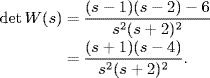
So, by Theorem 2.8, the system has three poles: two at s = 0 and one at s = − 2. And by Theorem 2.12, the zero polynomial of the system is z(s) = s − 5. Note that there is a pole-zero cancelation at s = − 2 when calculating the determinant of W(s).
The next example shows that even if a multivariable system has a pole and a zero at the same place, it does not mean that there must be a pole-zero cancelation.
Example 2.14 Consider the transfer function matrix
(2.40) ![]()
By Theorem 2.8, W(s) has poles at s = 0 and s = − 2. We also notice that W(s) loses rank at s = 0 and s = − 2. So, s = 0 and s = − 2 are also zeros of W(s), but there is no pole-zero cancelation.
If W(s) loses rank for any value of the complex variable s, by Definition 2.10 or Theorem 2.12, it does not mean that W(s) has (transmission) zeros at any place in the complex plane. However, such a “non-existing” zero may also cause a pole-zero cancelation. Sometimes, we call such a zero an invariant zero.
Example 2.15 Let
![]()
By Definition 2.10, both W1(s) and W2(s) have no zero. Now, let us check the poles of W1(s) and W2(s). By Theorem 2.8, W1(s) has only a single pole at s = 0 but W2(s) has double poles at s = 0. Where is another “pole” s = 0 for W1(s)? It may be assumed that the pole is canceled by an invariant zero at s = 0 because det W(s) = 0 for any value of s including zero, although such a zero is not counted by Definition 2.10.
Now, we consider the poles of the cascaded system W1(s)W2(s). At the first look, one may guess that the cascaded system has triple poles at s = 0. But, since
![]()
is singular for any complex variable s, by Theorem 2.8, we know that W1(s)W2(s) only has double poles at s = 0. The third pole at s = 0 is canceled again by the invariant zero.
Invariant zeros are actually caused by the singularity of system matrices. Note that in consensus problems, which will be discussed in Chapter 6 and Chapter 7, open-loop transfer function matrices are usually singular for any complex variable since the Laplacian matrix is singular.
2.4 Frequency-Domain Criteria of Stability
The return difference equation of the closed-loop system shown in Figure 2.2 is
(2.41) ![]()
According to linear system theory (Chen 1984; Desoer and Vidyasagar 1975), it holds that
where ϕc(s) is the characteristic polynomial (or quasi-polynomial for time-delayed systems) of the closed-loop system, and ϕo(s) is the characteristic polynomial (or quasi-polynomial for time-delayed systems) of the open-loop system. ![]() is referred to as the open-loop transfer function of the system. For the purpose of the well-posedness of the system we always assume that
is referred to as the open-loop transfer function of the system. For the purpose of the well-posedness of the system we always assume that
![]()
Equation (2.42) shows that the solutions of the following equation
may be a proper subset of the poles of the closed-loop system since cancelations may occur on the right side of (2.42). Nevertheless, if there is no cancelation between RHP pole(s) of the closed-loop system and RHP pole(s) of the open-loop system, the system is stable if and only if all the solutions of the equation (2.43) have strictly negative real parts.
Exercises2.16 Let the transfer function matrix W(s) be given by (2.14). Show that if
![]()
then (1) W(s)→ ∞ as s→ ∞, (2) the closed-loop system does not have a state representation in the standard form (A, B, C, D).
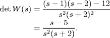
2.4.1 Loop Transformation and Multiplier
For a given closed-loop system, one can make some loop transformation as shown by Figure 2.6 for stability analysis. Obviously, we have
![]()
which yields the conclusion that
![]()
if and only if
![]()
and
![]()
where ![]() denotes a region in the complex plane, which can be
denotes a region in the complex plane, which can be ![]() ,
, ![]() , or
, or ![]() depending on the stability requirement. Therefore, if the feedback system composed of G1(s) and K(s) is (semi-)stable, the system shown by Figure 2.6(a) has the same (semi-)stability property as the system shown in Figure 2.6(b).
depending on the stability requirement. Therefore, if the feedback system composed of G1(s) and K(s) is (semi-)stable, the system shown by Figure 2.6(a) has the same (semi-)stability property as the system shown in Figure 2.6(b).
One can also introduce some multiplier into the loop as shown by Figure 2.7 and Figure 2.8.
Figure 2.6 (a) Original feedback system; (b) System with loop transformation.
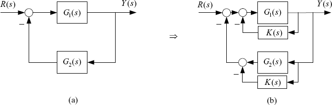
Figure 2.7 (a) Original feedback system; (b) System with multiplier.
Figure 2.8 (a) Original feedback system; (b) System with mixed loop transformation.
Loop transformation is a very useful tool in the analysis of the stability of feedback systems. When we apply some stability criteria such as the Nyquist criterion, ignorance of pole cancelations between the open-loop transfer function and the closed-loop transfer function may result in incorrect results as we will show later in this chapter. Proper loop transformation can remove such cancelations because it changes open-loop transfer functions. Moreover, since some stability criteria such as spectral radius theorem, small-gain theorem and passivity theorem (positive realness theorem) provide only sufficient conditions of stability and hence are conservative, loop transformations and multipliers change open-loop transfer functions and are helpful in reducing the conservatism of these stability criteria.
2.4.2 Multivariable Nyquist Stability Criterion
The stability test for closed-loop systems can be performed by use of frequency-domain techniques based on the multivariable (or generalized) Nyquist stability criterion. The following theorem is a modified version of the generalized Nyquist stability criterion which has been widely used in references (see, e.g., Vidyasagar (1985).
Theorem 2.17 Consider a system with an open-loop transfer function ![]() which has η RHP poles. Then, the closed-loop system has no RHP poles if and only if the Nyquist diagram of
which has η RHP poles. Then, the closed-loop system has no RHP poles if and only if the Nyquist diagram of ![]()
Remark 1. By the Nyquist diagram or the Nyquist plot of ![]() we mean the image of
we mean the image of ![]() as s goes clockwise around the Nyquist D-contour. The Nyquist D-contour includes the entire jω-axis and an infinite semi circle into the right-half plane. If
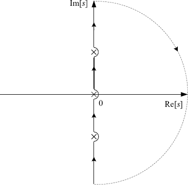
as s goes clockwise around the Nyquist D-contour. The Nyquist D-contour includes the entire jω-axis and an infinite semi circle into the right-half plane. If ![]() has jω-axis poles, one can use the D-contour illustrated in Figure 2.9 to avoid these poles by making sufficiently small semi circles into the RHP around them. By using such a D-contour the jω-axis poles of
has jω-axis poles, one can use the D-contour illustrated in Figure 2.9 to avoid these poles by making sufficiently small semi circles into the RHP around them. By using such a D-contour the jω-axis poles of ![]() are obviously excluded from the number of RHP poles of the open-loop system, which are sometimes briefly referred to as open-loop RPH poles (note that the “open-loop RHP pole” is not equal to the “open RHP pole”!). Since this D-contour goes around jω-axis poles of
are obviously excluded from the number of RHP poles of the open-loop system, which are sometimes briefly referred to as open-loop RPH poles (note that the “open-loop RHP pole” is not equal to the “open RHP pole”!). Since this D-contour goes around jω-axis poles of ![]() in the anti-clockwise direction, when drawing the Nyquist plot of
in the anti-clockwise direction, when drawing the Nyquist plot of ![]() one should add a semi circle with an infinite radius in the clockwise direction to connect the undefined part of the plot corresponding to each jω-axis pole. In this way, the jω-axis poles of the open-loop system are not regarded as “RHP poles”. So, the term “RHP poles” in the theorem actually should be understood as “open RHP poles”. If there is no cancelation of any of the jω-axis poles between the open-loop transfer function and the closed-loop transfer function, conditions (1) and (2) imply stability. Otherwise, only semi-stability is ensured.
one should add a semi circle with an infinite radius in the clockwise direction to connect the undefined part of the plot corresponding to each jω-axis pole. In this way, the jω-axis poles of the open-loop system are not regarded as “RHP poles”. So, the term “RHP poles” in the theorem actually should be understood as “open RHP poles”. If there is no cancelation of any of the jω-axis poles between the open-loop transfer function and the closed-loop transfer function, conditions (1) and (2) imply stability. Otherwise, only semi-stability is ensured.
Figure 2.9 D-contour excluding jω-axis poles.
Remark 2. The theorem itself does not tell if there is any RHP pole cancelation between the closed-loop system and the open-loop system. In Chapter 7 we will discuss how to justify if there exist multiple pole cancelations between the closed-loop system and the open-loop system at s = 0.
Remark 3. Since loop-transformation changes the open-loop transfer function but does not change the closed-loop transfer function, one can also use some loop transformation to avoid pole-zero cancelations of open-loop transfer functions and get the correct conclusion on the stability of the closed-loop system.
We use the following example to illustrate Theorem 2.17 and the associated remarks as well.
Example 2.18 Let ![]() , where
, where ![]() , and
, and ![]() By Theorem 2.8 we know that
By Theorem 2.8 we know that ![]() has a single pole at s = 0. Actually, as we have shown in Example 2.15, there is another open-loop pole at s = 0 which is canceled because det A = 0. Using the modified Nyquist D-contour given in Figure 2.9, the poles at s = 0 are not regarded as the RHP poles of
has a single pole at s = 0. Actually, as we have shown in Example 2.15, there is another open-loop pole at s = 0 which is canceled because det A = 0. Using the modified Nyquist D-contour given in Figure 2.9, the poles at s = 0 are not regarded as the RHP poles of ![]() . So we have η = 0. Because
. So we have η = 0. Because
![]()
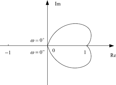
we can draw the Nyquist plot of ![]() as shown in Figure 2.10. In the plot we see that it neither passes through nor encircles the origin. Therefore, one may conclude that the closed-loop system has no RHP poles. But this does not lead to the conclusion that the system is stable. Instead, only the steady semi-stability can be derived, i.e., all the poles of the closed-loop system are inside the LHP or at s = 0.
as shown in Figure 2.10. In the plot we see that it neither passes through nor encircles the origin. Therefore, one may conclude that the closed-loop system has no RHP poles. But this does not lead to the conclusion that the system is stable. Instead, only the steady semi-stability can be derived, i.e., all the poles of the closed-loop system are inside the LHP or at s = 0.
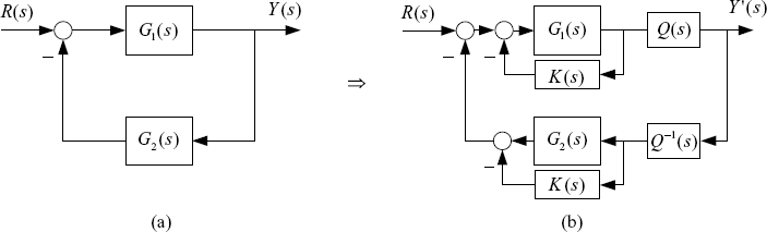
We can investigate the stability of this system by making a loop transformation. The system diagram is sketched in Figure 2.11(a). It can be transformed into the form given by Figure 2.11(c). From Figure 2.11(c) we have the transfer function matrix of the open-loop system as ![]() and
and ![]() . Therefore, we have η = 0. The Nyquist plot of
. Therefore, we have η = 0. The Nyquist plot of ![]() is given in Figure 2.12. It passes through the origin, and thus, the system is just marginally stable. The conclusion is the same as that obtained from the original diagram.
is given in Figure 2.12. It passes through the origin, and thus, the system is just marginally stable. The conclusion is the same as that obtained from the original diagram.
Figure 2.10 Nyquist plots without s = 0 as an open-loop RHP pole.
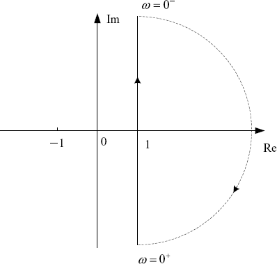
Figure 2.11 Transformation of system diagram.
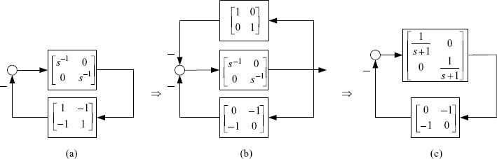
Figure 2.12 Nyquist plot of the transformed system.
As is well known, a great virtue of the classic Nyquist stability criterion is that it checks the closed-loop system stability by inspection of the Nyquist diagram of the open-loop transfer function. For SISO systems, Theorem 2.17 reduces to the classical Nyquist criterion since ![]() . For the multivariable systems, however, this theorem requires a plot of
. For the multivariable systems, however, this theorem requires a plot of ![]() . Desoer and Wang (1980) proved a version of the generalized Nyquist stability criterion which checks the stability of the closed-loop system by inspection of the eigenloci of the open-loop system.
. Desoer and Wang (1980) proved a version of the generalized Nyquist stability criterion which checks the stability of the closed-loop system by inspection of the eigenloci of the open-loop system.
The eigenloci are defined as the set of all the eigenvalues of the frequency response of the open-loop transfer function matrix, ![]() , as jω goes clockwise around the Nyquist D-contour. Note that, unlike the SISO case, in general
, as jω goes clockwise around the Nyquist D-contour. Note that, unlike the SISO case, in general ![]() is not a rational function of s, and hence the conjugate property does not hold, i.e.,
is not a rational function of s, and hence the conjugate property does not hold, i.e.,
![]()
This leads to the fact that a single eigenlocus ![]() may not form a closed path when ω varies from −∞ to ∞. Fortunately, when λi(s) is irrational on s, there always exists another eigenvalue λi+1(s) which is conjugate with λi(s), i.e.,
may not form a closed path when ω varies from −∞ to ∞. Fortunately, when λi(s) is irrational on s, there always exists another eigenvalue λi+1(s) which is conjugate with λi(s), i.e.,
![]()
Hence, the part of the eigenlocus ![]() is conjugate with the part of the eigenlocus
is conjugate with the part of the eigenlocus ![]() , and the part of the eigenlocus
, and the part of the eigenlocus ![]() is conjugate with the part of the eigenlocus
is conjugate with the part of the eigenlocus ![]() . Therefore, when ω varies from −∞ to ∞, the eigenloci of
. Therefore, when ω varies from −∞ to ∞, the eigenloci of ![]() and
and ![]() form two closed paths. In such a way, we can count the times in which the eigenloci
form two closed paths. In such a way, we can count the times in which the eigenloci ![]() , enclose the point (− 1, j0).
, enclose the point (− 1, j0).
Let N be the sum of the times in which the eigenloci ![]() , enclose the point (− 1, j0) anticlockwise as jω goes clockwise around the Nyquist D-contour. Then, the generalized Nyquist stability criterion can be stated as follows.
, enclose the point (− 1, j0) anticlockwise as jω goes clockwise around the Nyquist D-contour. Then, the generalized Nyquist stability criterion can be stated as follows.
Theorem 2.19 Consider a system with an open-loop transfer function ![]() which has η open RHP poles. Then, the closed-loop system has no open RHP poles if and only if
which has η open RHP poles. Then, the closed-loop system has no open RHP poles if and only if
Furthermore, if there is no cancelation of jω-axis poles between the open-loop system and the closed-loop system, the closed-loop system is stable.
Remark. The assumption of no cancelation of jω-axis poles between the open-loop system and the closed-loop system can always be satisfied by introducing a proper loop transformation.
For many network-based distributed control systems, open-loop systems composed of agents have no open RHP poles. The following theorem, which is actually a corollary of Theorem 2.19, is very useful for such systems.
Theorem 2.20 Suppose that the open-loop transfer function ![]() has no open RHP poles. Then, the closed-loop system has no open RHP poles if and only if the eigenloci
has no open RHP poles. Then, the closed-loop system has no open RHP poles if and only if the eigenloci ![]() , do not enclose the point (− 1, j0) as jω goes clockwise around the Nyquist D-contour. Furthermore, if there is no cancelation of jω-axis poles between the open-loop system and the closed-loop system, the closed-loop system is stable.
, do not enclose the point (− 1, j0) as jω goes clockwise around the Nyquist D-contour. Furthermore, if there is no cancelation of jω-axis poles between the open-loop system and the closed-loop system, the closed-loop system is stable.
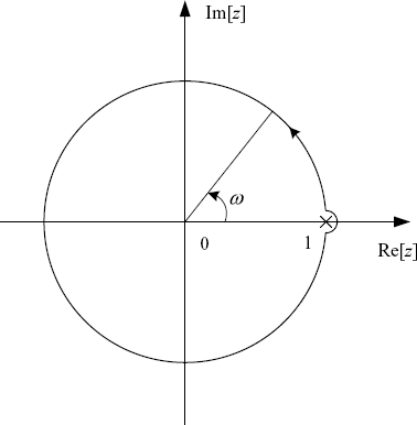
Theorem 2.17, Theorem 2.19 and Theorem 2.20 can be easily extended to discrete-time systems after replacing the D-contour by the unit circle in the complex plane. Note that if the z-transfer function matrix ![]() of the open-loop system has a pole just on the unit circle, the unit circle should be modified by making a sufficiently small semi circle into the region outside the unit circle around the pole (see Figure 2.13).
of the open-loop system has a pole just on the unit circle, the unit circle should be modified by making a sufficiently small semi circle into the region outside the unit circle around the pole (see Figure 2.13).
Figure 2.13 Modified unit circle.
For convenience of statement, we denote by ![]() the interior of the unit disc (briefly as IUD), i.e.,
the interior of the unit disc (briefly as IUD), i.e., ![]() . The closure of
. The closure of ![]() is denoted by
is denoted by ![]() and briefly referred to as the closed IUD. We also denote by
and briefly referred to as the closed IUD. We also denote by ![]() the closed outer part of the unit disc (briefly as OUD), i.e.,
the closed outer part of the unit disc (briefly as OUD), i.e., ![]() and denote by
and denote by ![]() the open outer part of the unit disc (briefly as the open OUD), i.e.,
the open outer part of the unit disc (briefly as the open OUD), i.e., ![]() .
.
Definition 2.21 Let ϕ(z) be the pole (quasi-)polynomial of a discrete-time. The system is said to be stable if
(2.44) ![]()
The system is said to be semi-stable if all its poles are in
(2.45) ![]()
In particular, it is said to be steady semi-stable if
(2.46) ![]()
Then, the discrete-time analog of Theorem 2.20 can be stated as follows. The discrete-time analogs of the other versions of the generalized Nyquist stability criterion are similar.
Theorem 2.22 Suppose that the open-loop transfer function ![]() of a discrete-time system has no open OUD poles. Then, the closed-loop system has no open OUD poles if and only if the eigenloci
of a discrete-time system has no open OUD poles. Then, the closed-loop system has no open OUD poles if and only if the eigenloci ![]() , do not enclose the point (− 1, j0) as ω varies from −π to π. Furthermore, if there is no cancelation of unit-circle poles between the open-loop system and the closed-loop system, the closed-loop system is stable.
, do not enclose the point (− 1, j0) as ω varies from −π to π. Furthermore, if there is no cancelation of unit-circle poles between the open-loop system and the closed-loop system, the closed-loop system is stable.
2.4.3 Spectral Radius Theorem and Small-Gain Theorem
Using the generalized Nyquist stability criterion, Theorem 2.17, it can be proved that the stability of a closed-loop system with a stable open-loop transfer function can be verified by testing the spectral radius of the open-loop transfer function at each frequency, which is defined as the maximum eigenvalue magnitude, i.e.,
(2.47) ![]()
Theorem 2.23 Consider a system with a stable open-loop transfer function ![]() . Then, the closed-loop system is stable if
. Then, the closed-loop system is stable if
(2.48) ![]()
This theorem which is referred to as the spectral radius theorem was proved in Skogestad and Postlethwaite (1996). With some modification of the proof we can prove the following extended spectral radius theorem for the test of steady semi-stability and marginal stability.
Theorem 2.24 Consider a system with a stable open-loop transfer function ![]() . Then, the closed-loop system is steady semi-stable, if
. Then, the closed-loop system is steady semi-stable, if
(2.49) ![]()
Moreover, if ![]() , and
, and ![]() , then the closed-loop system is marginally stable with s = 0 as a simple pole.
, then the closed-loop system is marginally stable with s = 0 as a simple pole.
Proof. Firstly, we note that the closed-loop system has no pure imaginary poles because ![]() .
.
Secondly, we prove that the closed-loop system has no open RHP poles. We prove this by contradiction. Suppose that it has at least one open RHP pole. By the generalized Nyquist theorem (Theorem 2.17), ![]() must enclose the origin, which implies that there exists an
must enclose the origin, which implies that there exists an ![]() such that
such that ![]() . Then, there exists a gain
. Then, there exists a gain ![]()
![]() (0, 1) such that
(0, 1) such that
(2.50) ![]()
because ![]() for
for ![]() = 0. Then, the following derivation leads a contradiction:
= 0. Then, the following derivation leads a contradiction:
(2.51) ![]()
(2.52) ![]()
(2.53) ![]()
(2.54) ![]()
(2.55) ![]()
Based on the above discussion we conclude that the closed-loop system is steady semi-stable.
Thirdly, ![]() implies that the closed-loop system has at least one pole at s = 0. Now, we show that any possible pole of the closed-loop system at s = 0 must be simple. Indeed, let us consider poles of a perturbed system with characteristic equation
implies that the closed-loop system has at least one pole at s = 0. Now, we show that any possible pole of the closed-loop system at s = 0 must be simple. Indeed, let us consider poles of a perturbed system with characteristic equation
(2.56) ![]()
where ![]()
![]() (0, 1). Obviously,
(0, 1). Obviously, ![]() , for all
, for all ![]() including ω = 0 because
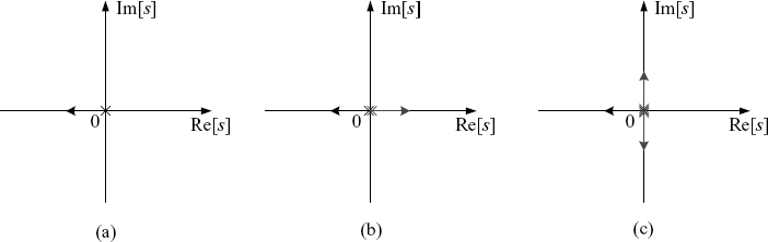
including ω = 0 because ![]() = 1. So, by Theorem 2.23 the perturbed system is stable. By the rule of root locus (Nise (2000), root loci for perturbed systems with simple pole, double poles and triple poles, respectively, at s = 0 are shown in Figure 2.14. It is clear that only the case of simple pole can be stable.
= 1. So, by Theorem 2.23 the perturbed system is stable. By the rule of root locus (Nise (2000), root loci for perturbed systems with simple pole, double poles and triple poles, respectively, at s = 0 are shown in Figure 2.14. It is clear that only the case of simple pole can be stable.
Figure 2.14 Root locus near s = 0: (a) simple pole, (b) double poles, (c) triple poles.
Note that the open-loop system ![]() in the above theorem may be obtained based on some loop transformation.
in the above theorem may be obtained based on some loop transformation.
Example 2.25 Let us consider the system given in Example 2.18 again. After the loop transformation shown by Figure 2.11 we have
![]()
It is easy to check that
![]()
and ![]() . So, the closed-loop system has no RHP poles except for a simple pole at s = 0, and hence, is marginally stable.
. So, the closed-loop system has no RHP poles except for a simple pole at s = 0, and hence, is marginally stable.
If we choose a matrix norm satisfying ||AB|| ≤ ||A|| · ||B||, we have ![]() . Then, some small-gain theorems can be directly obtained from Theorem 2.23 and Theorem 2.24 as follows.
. Then, some small-gain theorems can be directly obtained from Theorem 2.23 and Theorem 2.24 as follows.
Theorem 2.26 Consider a system with a stable open-loop transfer function ![]() . Then, the closed-loop system is stable if
. Then, the closed-loop system is stable if
(2.57) ![]()
Theorem 2.27 Consider a system with a stable open-loop transfer function ![]() . Then, the closed-loop system has all poles in the LHP except for a simple pole at s = 0 and hence is marginally stable, if
. Then, the closed-loop system has all poles in the LHP except for a simple pole at s = 0 and hence is marginally stable, if
(2.58) ![]()
(2.59) ![]()
2.4.4 Positive Realness Theorem
According to the generalized Nyquist stability criterion, Theorem 2.17, one can also analyze the stability of the closed-loop system by testing the positive realness of the eigenvalues of the transfer function matrix.
Theorem 2.28 Consider a system with a stable open-loop transfer function ![]() . Then, the closed-loop system is stable if
. Then, the closed-loop system is stable if
(2.60) ![]()
With slight modification of the proof of Theorem 2.24 one can also obtain the following theorem for the test of marginal stability.
Theorem 2.29 Consider a system with a stable open-loop transfer function ![]() . Then, the closed-loop system has all poles in the LHP except for a simple pole at s = 0 and hence is marginally stable, if
. Then, the closed-loop system has all poles in the LHP except for a simple pole at s = 0 and hence is marginally stable, if
(2.61) ![]()
(2.62) ![]()
2.5 Scalable Stability Criteria
2.5.1 Estimation of Spectrum of Complex Matrices
To apply Theorem 2.17 or Theorem 2.19 it is necessary to get the eigenloci ![]() . Generally, there is no analytical formula for calculating eigenvalues of matrices. The following lemmas can be used for the estimation of the spectrum of
. Generally, there is no analytical formula for calculating eigenvalues of matrices. The following lemmas can be used for the estimation of the spectrum of ![]() denoted by σ(A): = {λ1(A),
denoted by σ(A): = {λ1(A), ![]() , λn(A)}.
, λn(A)}.
The first lemma is usually called Gershgorin's disc lemma (Horn and Johnson (1985).
Lemma 2.30 For any ![]() it holds
it holds
(2.63) ![]()
where
Remark. The eigenvalues of A are also in the union of the discs:
(2.65) ![]()
From (2.64) it follows that ![]() , which implies that any complex number in the disk Di has the absolute value less than or equal to the sum of the absolute values of the entries of the same row. So, the following corollary is straightforward.
, which implies that any complex number in the disk Di has the absolute value less than or equal to the sum of the absolute values of the entries of the same row. So, the following corollary is straightforward.
Corollary 2.31 For any ![]() it holds
it holds
(2.66) 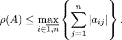
Define
(2.67) ![]()
where ![]() . We have ρ(A) = ρ(HAH−1) for
. We have ρ(A) = ρ(HAH−1) for ![]() . Based on this fact we get the following corollary of Gershgorin's disc lemma for reducing the conservatism of Corollary 2.31
. Based on this fact we get the following corollary of Gershgorin's disc lemma for reducing the conservatism of Corollary 2.31
Corollary 2.32 For any ![]() it holds
it holds
(2.68) 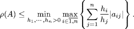
Let ![]() and ξ*ξ = 1. Then, for any eigenvalue λi of A we have λi = λiξ*ξ = ξ*Aξ. So, by defining the field of values of A as follows (Horn and Johnson (1991):
and ξ*ξ = 1. Then, for any eigenvalue λi of A we have λi = λiξ*ξ = ξ*Aξ. So, by defining the field of values of A as follows (Horn and Johnson (1991):
(2.69) ![]()
the following lemma is obvious.
Lemma 2.33 For any ![]() , it holds
, it holds
(2.70) ![]()
If the complex matrix A can be written as a product of a diagonal matrix and a Hermitian matrix, then its spectrum can be further estimated by Vinnicombe's lemma (Vinnicombe (2000), which can be derived from Lemma 2.33.
Lemma 2.34 Let ![]() , Q = Q* ≥ 0 and
, Q = Q* ≥ 0 and ![]() . Then,
. Then,
(2.71) ![]()
where ρ(·) denotes the matrix spectral radius, and Co(·) the convex hull.
Proof. Denote by N(A) the null space of the complex matrix A. Then,
So, we have
![]()
which implies that ![]() . The lemma is thus proved.
. The lemma is thus proved.
Remark. The lemma was proved by Vinnicombe (2000) for the case of Q = Q* > 0. The current form of the lemma and the proof are given by Lestas and Vinnicombe (2005).
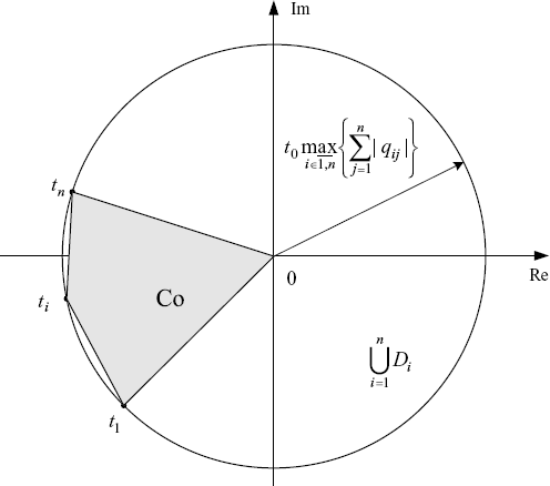
The following example illustrates that in most cases Vinnicombe's lemma is much less conservative than Gershgorin's disc lemma if A is a product of a diagonal matrix and a Hermitian matrix.
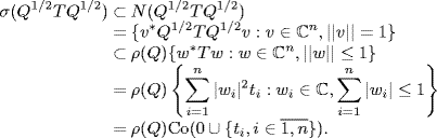
Example 2.35 Suppose ![]() , and
, and ![]() is a Hermitian matrix with zero as diagonal entries, i.e., qii = 0. Then, by Gershgorin's disc lemma we have
is a Hermitian matrix with zero as diagonal entries, i.e., qii = 0. Then, by Gershgorin's disc lemma we have
Now, by using Vinnicombe's lemma and Corollary 2.31 of Gershgorin's disc lemma we get
![]() is a disc centered at the origin with radius as
is a disc centered at the origin with radius as ![]() . Co is a convex polygon contained in the disc as shown by Figure 2.15. Obviously, the higher the diversity degree of θi is, the closer the two regions are.
. Co is a convex polygon contained in the disc as shown by Figure 2.15. Obviously, the higher the diversity degree of θi is, the closer the two regions are.
Figure 2.15 Comparison of Gershgorin's lemma and Vinnicombe's lemma.
2.5.2 Scalable Stability Criteria for Asymmetric Systems
Now, we consider the stability of the distributed control system described by (2.1), (2.2) and (2.3), which is shown by Figure 2.2. For convenience, let us re-sketched the diagram of the system as shown by Figure 2.16, where Λ(s) is defined by (2.11) and A(s) is defined by (2.12). The following theorem is a direct consequence of the spectral radius theorem and Gershgorin's disc lemma.
Figure 2.16 Distributed control system.
Theorem 2.36 Suppose Gi(s), ![]() , have no open RHP poles. The closed-loop system shown by Figure 2.16 has no open RHP poles, and hence is semi-stable if
, have no open RHP poles. The closed-loop system shown by Figure 2.16 has no open RHP poles, and hence is semi-stable if
Furthermore, if there is no cancelation of jω-axis poles between the open-loop system and the closed-loop system, the closed-loop system is stable.
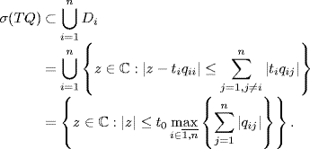
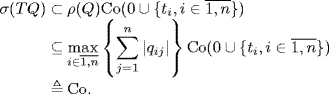
Proof. Denote by H(s) the upper part of the system as shown by Figure 2.16, i.e.,
Then, the open-loop transfer function of the system can be written as diag{Hi(s)}A(s). By Theorem 2.20, the closed-loop system has no open RHP poles if and only if the eigenloci
![]()
do not enclose the point (− 1, j0) for m = 1, ![]() , n as ω varies from 0 to infinity. By Lemma 2.30, the spectrum of
, n as ω varies from 0 to infinity. By Lemma 2.30, the spectrum of ![]() is contained in the union of the following discs:
is contained in the union of the following discs:
Obviously, the eigenloci ![]() do not enclose (− 1, j0) if
do not enclose (− 1, j0) if
![]()
which is equivalent to (2.72). Therefore, the closed-loop system does indeed have no open RHP poles. If there is no cancelation of jω-axis poles between the open-loop system and the closed-loop system, by Theorem 2.20 again, the closed-loop system is stable.
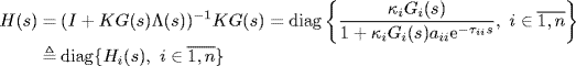
Theorem 2.36 gives a sufficient stability condition which is independent of communication delays τij, i ≠ j. But it still depends on the self-delays τii. However, if we replace e−jωτii by a unit disc ![]() , then a sufficient condition for (2.72) is given by the following corollary.
, then a sufficient condition for (2.72) is given by the following corollary.
Corollary 2.37 Suppose Gi(s), ![]() , have no open RHP poles. The closed-loop system shown by Figure 2.16 has no open RHP poles if
, have no open RHP poles. The closed-loop system shown by Figure 2.16 has no open RHP poles if
Furthermore, if there is no cancelation of jω-axis poles between the open-loop system and the closed-loop system, the closed-loop system is stable.
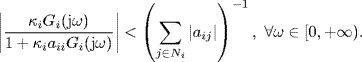
This is a more conservative condition but it is independent of self-delays. The geometric meaning of condition (2.73) can be illustrated as follows: all the circle centered at the Nyquist plot of κiaiiGi(jω) with radius ![]() is inside but does not touch the unit disc (see Figure 2.17).
is inside but does not touch the unit disc (see Figure 2.17).
Figure 2.17 Geometrical illustration of Corollary 2.37.
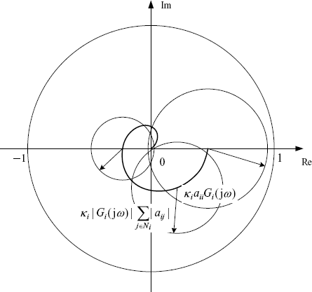
Figure 2.17 clearly shows that the condition (2.73) can be satisfied only if ![]() . In the other hand, if
. In the other hand, if ![]() , it can be shown that there always exist local proportional controls stabilizing the system.
, it can be shown that there always exist local proportional controls stabilizing the system.
Corollary 2.38 Suppose ![]() ,
, ![]() . Then, the system shown by Figure 2.16 is stable if control gains
. Then, the system shown by Figure 2.16 is stable if control gains ![]() , are sufficiently small.
, are sufficiently small.
Proof. Since Gi(s) has no jω-axis poles, we know that |Gi(jω)| is bounded for all ![]() . Therefore,
. Therefore,
![]()
This implies that (2.72) is always satisfied if ![]() , are sufficiently small.
, are sufficiently small.
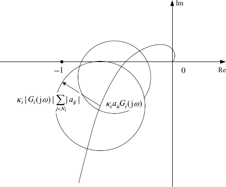
Remark. If all self-delays are zero, i.e. τii = 0, the condition (2.72) reduces to
This condition does not require ![]() (see Figure 2.18 for illustration).
(see Figure 2.18 for illustration).
Figure 2.18 Geometrical illustration of Theorem 2.36 for the case τii = 0.
For the case when the transfer function of the open-loop system is stable, by applying Theorem 2.24 and the argument similar to the proof of Theorem 2.36, we can get the following scalable criterion for the test of the steady semi-stability and the marginal stability.
Theorem 2.39 Suppose ![]() ,
, ![]() . The closed-loop system shown by Figure 2.16 is steady semi-stable if
. The closed-loop system shown by Figure 2.16 is steady semi-stable if
(2.74) 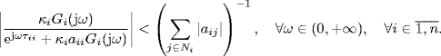
Moreover, if ρ(diag{Hi(0)}A(0)) = 1, and det (I + diag{Hi(0)}A(0)) = 0, then the closed-loop system is marginally stable with s = 0 as a simple pole.
2.5.3 Scalable Stability Criteria for Symmetric Systems
Since ![]() , the system in Figure 2.2 can be re-sketched in Figure 2.19. Recall that the system is said to be symmetric if
, the system in Figure 2.2 can be re-sketched in Figure 2.19. Recall that the system is said to be symmetric if ![]() .
.
Figure 2.19 Distributed control system.
For symmetric systems one can get some scalable stability criterion that is less conservative than Theorem 2.36.
Theorem 2.40 Suppose ![]() and Gi(s) has no open RHP poles. Let γi be the gain margin of the stable transfer function Gi(s), and
and Gi(s) has no open RHP poles. Let γi be the gain margin of the stable transfer function Gi(s), and ![]() . Then, the closed-loop system shown by Figure 2.19 has no open RHP poles if the following conditions are satisfied for all ω ≥ 0:
. Then, the closed-loop system shown by Figure 2.19 has no open RHP poles if the following conditions are satisfied for all ω ≥ 0:
Furthermore, if there is no cancelation of jω-axis poles between the open-loop system and the closed-loop system, the closed-loop system is stable.
Proof. We just prove the semi-stability part. The stability part follows directly from Theorem 2.20.
By Theorem 2.20, the closed-loop system has no RHP poles if and only if the eigenloci
![]()
do not enclose the point (− 1, j0) for m = 1, ![]() , n as ω varies from 0 to infinity. Note that
, n as ω varies from 0 to infinity. Note that
![]()
And moreover, ![]() because
because ![]() . Therefore, by Lemma 2.34, the closed-loop system has no open RHP poles if
. Therefore, by Lemma 2.34, the closed-loop system has no open RHP poles if
![]()
The above condition is satisfied if
(2.75) ![]()
and
Since the spectral radius of any matrix is bounded by its maximum absolute row sum, (2.76) is satisfied if condition (2) of the theorem holds. Thus, the theorem is proved.
If we use Corollary 2.32 instead of Corollary 2.31 of Gershgorin's disc lemma in the proof, we can get the following result for reducing the conservatism of Theorem 2.40.
Theorem 2.41 Suppose ![]() and Gi(s) has no open RHP poles. The closed-loop system shown by Figure 2.19 has no open RHP poles if there exist positive real numbers
and Gi(s) has no open RHP poles. The closed-loop system shown by Figure 2.19 has no open RHP poles if there exist positive real numbers ![]() such that the following conditions are satisfied for all ω ≥ 0:
such that the following conditions are satisfied for all ω ≥ 0:
Furthermore, if there is no cancelation of jω-axis poles between the open-loop system and the closed-loop system, the closed-loop system is stable.
If the condition
in the above theorem is satisfied, the second condition in Theorem 2.40 or Theorem 2.41 gives a local and hence scalable test for the stability. Therefore, condition (2.77) can be considered as a scalability condition. Note that the scalability condition (2.77) does not necessarily hold even if each Nyquist plot ![]() does not contain (− 1, j0). This problem will be studied in the next chapter.
does not contain (− 1, j0). This problem will be studied in the next chapter.
Exercises 2.42 Let
![]()
and
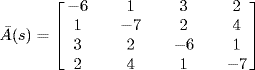
in the system shown by Figure 2.19. Derive scalable semi-stability conditions by Theorem 2.36, Theorem 2.40 and Theorem 2.41, respectively. Compare the conservatism of the obtained conditions with the help of a simulation toolbox (e.g., MATLAB®).
2.5.4 Robust Stability in Deformity of Symmetry
Symmetry of is such a fragile property that may be easily destroyed by small perturbations. Many factors in practical systems, such as uncertainty of agent dynamics, diversity of communication delays or heterogeneousness of channel dynamics, may lead to deformity of the symmetry defined by Definition 2.2 Therefore, any analysis or design method based on the assumption of the system symmetry must be robust against perturbations. Fortunately, the robust control theory can help us to extend the scalable stability criteria to most cases of deformity of symmetry.
Let us consider the case when there are some uncertainties in communication channels that cause the asymmetry of the system, as shown by Figure 2.20. Here, we assume that the nominal system, i.e., the system with ΔA(s) = 0, is symmetric. Suppose that the uncertainty matrix ΔA(s) is subject to the following structural constraint:
where ![]() and
and ![]() are some constant matrices that describe the structure of the uncertainty, Δ(s) satisfies the following condition:
are some constant matrices that describe the structure of the uncertainty, Δ(s) satisfies the following condition:
where ![]() is a known function of ω. Then, by loop transformation we can equivalently transform the system into an interconnection form shown by Figure 2.21 with
is a known function of ω. Then, by loop transformation we can equivalently transform the system into an interconnection form shown by Figure 2.21 with
![]()
According to the robust control theory (see, e.g., Feng, Tian and Xin 1996, Zhou, Doyle and Glover (1996)), under the assumption that
the asymmetric uncertain system shown by Figure 2.20 is robustly stable if and only if
We summarize the conclusion of the above discussion in the following theorem.
Figure 2.20 Distributed control system with uncertainty in network channels.
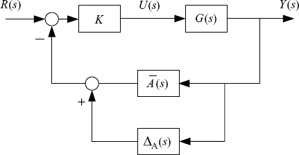
Figure 2.21 Symmetric system with asymmetric perturbations.
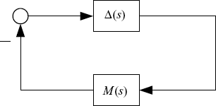
Theorem 2.43 Under the conditions (2.78), (2.79) and (2.80), the perturbed system shown by Figure 2.20 is robustly stable if and only if (2.81) holds.
Remark. A sufficient condition for ![]() is that
is that
Note that the left-hand side of (2.82) is just the nominal symmetric system. So, its stability can be checked by Theorem 2.40 or Theorem 2.41.
We can also consider the bipartite system with an additive uncertainty ΔP(s) in agent plants, as shown by Figure 2.22. Note that the uncertainty ΔP(s) may destroy the homogeneousness assumption (2.27), and hence, destroy the symmetry of the system. Suppose that ΔP(s) is subject to the following structural constraint:
where ![]() and
and ![]() describe the structure of the uncertainty, and Δ(s) satisfies the following condition:
describe the structure of the uncertainty, and Δ(s) satisfies the following condition:
where ![]() is a known function of ω. The system can also be equivalently transformed into the interconnection form shown by Figure 2.21 with
is a known function of ω. The system can also be equivalently transformed into the interconnection form shown by Figure 2.21 with
Similarly, we assume that
Then, we have the following result.
Figure 2.22 Distributed control system with uncertainty in agent plants.
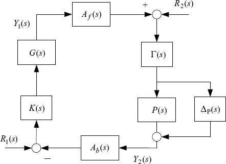
Theorem 2.44 Under the conditions (2.83), (2.84) and (2.86), the perturbed system shown by Figure 2.22 is robustly stable if and only if
(2.87) ![]()
where M(s) is given by (2.85).
2.6 Notes and References
Modeling of systems with forward and backward communication channels are discussed in many references on coordination control and congestion control (see, e.g., Arcak 2007; Low, Paganini and Doyle 2002; Wen and Arcak 2003). Using bipartite graphs to describe interconnection topologies of such systems and the symmetry analysis is new. The definitions of poles and zeros are given following MacFarlane and Karcanias (1976). Note that for multivariable systems there are various definitions of zeros, see MacFarlane and Karcanias (1976) and Rosenbrock (1973). For their computation, see Davison and Wang (1978) and Laub and Moore (1978). The difficulties associated with pole-zero cancelations in multivariable systems can be treated by state-space techniques using the concepts of controllability and observability. A pure algebraic approach to analyzing input-output properties including the equivalence between the systems after/before loop transformations can be found in more detail in the classic book of Desoer and Vidyasagar (1975), where general settings are used. The Nyquist stability was generalized in several ways for multivariable systems in the 1970s (Barman and Katzenelson 1974; Belletrutti and MacFarlane 1971; Callier and Desoer 1972; Davis 1972; Desoer and Vidyasagar 1975; MacFarlane and Postlethwaite 1977; Saeks 1975). Theorem 2.17 is taken from Vidyasagar (1985) while Theorem 2.19 adopts the result of Desoer and Vidyasagar (1975). Gershgorin's disc lemma has been a well-known tool for deriving scalable or decentralized stability results due to the study of frequency-domain analysis and design of multivariable systems by the so-called British school (Belletrutti and MacFarlane 1971; MacFarlane and Karcanias 1976; Rosenbrock 1970, 1974). Lemma 2.34 is a recent important contribution made by Vinnicombe (2000) to the estimation of the spectrum of complex matrices with application to the scalable stability analysis.
Arcak M (2007). Passivity as a design tool for group coordination. IEEE Transactions on Automatic Control, 52, 1380–1390.
Barman JF and Katzenelson J (1974). A generalized Nyquist-type stability criterion for multivariable feedback systems. International Journal of Control, 20(4), 593–622.
Belletrutti JJ and MacFarlane AGJ (1971). Characteristic loci techniques in multivariable control systems. Proc. Inst. Elec. Eng., 118, 1291–1297.
Callier FM and Desoer CA (1972). A graphical test for checking the stability of a linear time-invariant feedback systems. IEEE Transactions on Automatic Control, 17, 773–780.
Chen CT (1984). Linear System Theory and Design. CBS College Publishing, New York.
Davis JH (1972). Encirclement conditions for stability and instability of feedback control systems with delays. International Journal of Control, 15, 793–799.
Davison EJ (1983). Some properties of minimum phase systems and “square-down” systems. IEEE Transactions on Automatic Control, 28, 221–222.
Davison EJ and Wang SH (1978). An algorithm for the calculation of transmission zeros of (C,A,B,D) using high-gain output feedback. IEEE Transactions on Automatic Control, 23, 738–741.
Desoer CA and Vidyasagar M (1975). Feedback Systems: Input-Output Properties, Academic Press, New York.
Desoer CA and Wang Y-T (1980). On the generalized Nyquist Stability Criterion. IEEE Transactions on Automatic Control, 25(2), 187–196.
Feng C-B, Tian Y-P and Xin X (1996). Robust Control System Design (in Chinese). Southeast University Press, Nanjing.
Gu K, Kharitonov VL and Chen J (2003). Stability of Time-delayed Systems. Birkhäuser, Boston.
Horn RA and Johnson CR (1985). Matrix analysis, 1st edn. Cambridge University Press, New York.
Horn RA and Johnson CR (1991). Topics in Matrix analysis, 1st edn. Cambridge University Press, New York.
Laub AJ and Moore BC (1978). Calculation of transmission zeros using QZ techniques. Automatica, 14, 557–566.
Lestas I and Vinnicombe G (2005). Scalable robustness for consensus protocols with heterogeneous dynamics. Proceedings of IFAC world Congress, Prague.
Low SH, Paganini F and Doyle JC (2002). Internet congestion control. IEEE control systems Magazine, 22, 28–43.
MacFarlane AGJ and Karcanias N (1976). Poles and zeros of linear multivariable systems: a survey of algebraic, geometric and complex variable theory. International Journal of Control, Vol.24, 33–74.
MacFarlane AGJ and Postlethwaite I (1977). Generalized Nyquist stability criterion and multivariable root loci. International Journal of Control, 25(1), 81–127.
Nise NS (2000). Control Systems Engineering. 3rd ed., John Wiley & Sons, New York.
Rosenbrock HH (1970). State-space and Multivariable Theory. Nelson, London.
Rosenbrock HH (1973). The zeros of a system. International Journal of Control, 18, 297–299.
Rosenbrock HH (1974). Computer-Aided Control System Design. Academic Press, New York.
Saeks R (1975). On the encirclement condition and its generalization. IEEE Transactions on Circuits and Systems, 22, 780–785.
Skogestad S and Postlethwaite I (1996). Multivariable Feedback Control: Analysis And Design. John Wiley & Sons.
Vidyasagar M (1985). Control System Synthesis: A Factorization Approach. MIT Press.
Vinnicombe G (2000). On the stability of end-to-end congestion control for the Internet. Technical report CUED/F-INFENG/TR., No.398, 2000.
Wen JT and Arcak M (2003). A unifying passivity framework for network flow control. Proceedings of IEEE Infocom, San Francisco, California.
Zhou K, Doyle JC and Glover K (1996). Robust and Optimal Control. Prentice-Hall, Upper Saddle River, NJ.