
2
Single‐Integrator Model
This chapter will set the foundation for the formation control designs presented in the book. We use here a very simple model for the motion of the agents known as the single‐integrator model, which only includes two variables: position and velocity. This is a simplified kinematic model for omnidirectional robots (e.g., mobile robots with Swedish wheels 41). Specifically, we consider a system of ![]() agents governed by the first‐order differential equation
agents governed by the first‐order differential equation
where ![]() is the position and
is the position and ![]() is the velocity‐level control input of the
is the velocity‐level control input of the ![]() th agent with respect to an Earth‐fixed coordinate frame. The name “single integrator” originates from the fact that the transfer function matrix of (2.1) is
th agent with respect to an Earth‐fixed coordinate frame. The name “single integrator” originates from the fact that the transfer function matrix of (2.1) is
where ![]() is the Laplace variable, i.e., the inputs and outputs are separated by one integrator.
is the Laplace variable, i.e., the inputs and outputs are separated by one integrator.
Formation controllers based on ( 2.1 ) are called high‐level control laws because they are often embedded in controllers designed for more refined agent models. Therefore, the control laws introduced in this chapter will form the basis for all subsequent designs.
2.1 Formation Acquisition
We begin with the formation acquisition problem defined in Section 1.4. Given 2.1, we seek to design ![]() ,
, ![]() and
and ![]() , where
, where ![]() was defined in (1.2) to achieve the control objective described by (1.26) (or equivalently (1.27)).
was defined in (1.2) to achieve the control objective described by (1.26) (or equivalently (1.27)).
It is appropriate at this point to elaborate on an issue mentioned at the end of Section 1.3.6 regarding framework ambiguities. The inputs ![]() ,
, ![]() will directly control the distances
will directly control the distances ![]() ,
, ![]() . Therefore, they can only directly ensure that
. Therefore, they can only directly ensure that
which is equivalent to
Note that 2.3 is different than (1.27) since it is only defined for ![]() while (1.27) is defined for all
while (1.27) is defined for all ![]() . This is potentially problematic since (with abuse of notation)
. This is potentially problematic since (with abuse of notation) ![]() Iso
Iso![]() Amb
Amb![]() . Therefore, the control scheme will need to avoid the possibility that
. Therefore, the control scheme will need to avoid the possibility that ![]() Amb
Amb![]() as
as ![]() . This will be accomplished by initializing the agents sufficiently close to Iso
. This will be accomplished by initializing the agents sufficiently close to Iso![]() in the sense that dist
in the sense that dist![]() dist
dist![]() .
.
To simplify the notation in the following derivations, we define the relative position of two agents as
and let ![]() ,
, ![]() with the same ordering of terms as the edge function (1.7). The distance error is given by
with the same ordering of terms as the edge function (1.7). The distance error is given by
Note that (1.27) is equivalent to ![]() as
as ![]() ,
, ![]() . The distance error dynamics can be derived from 2.6 and 2.1 as
. The distance error dynamics can be derived from 2.6 and 2.1 as

Let
which can be rewritten as
using 2.6. Given that ![]() (or equivalently,
(or equivalently, ![]() ), it is not difficult to see that
), it is not difficult to see that ![]() if and only if
if and only if ![]() . We now introduce the following Lyapunov function candidate
. We now introduce the following Lyapunov function candidate

where ![]() and
and ![]() ,
, ![]() are ordered as (1.7). This function is positive definite in
are ordered as (1.7). This function is positive definite in ![]() and its level surfaces,
and its level surfaces, ![]() for some
for some ![]() , are closed since
, are closed since ![]() .
.
The time derivative of 2.10 along 2.7 is given by

Using (1.15), (1.16), and 2.9, 2.11 can be conveniently written as1
where ![]() is the stacked vector of control inputs.
is the stacked vector of control inputs.
Before presenting the main result, we introduce a lemma that establishes the relationship between Corollary 1.2 and the level surfaces of the Lyapunov function candidate.
The control law for solving the formation acquisition problem is given in the following theorem. Its structure is based on 2.12 and Lyapunov stability theory. Specifically, the goal is to make the time derivative of the Lyapunov function candidate negative definite 8.

Figure 2.1Energy landscape showing the two equilibrium points, Iso and Amb
 , at the bottom of each well.
The initial condition ![]() in Theorem 2.1 is a sufficient condition for the actual formation
in Theorem 2.1 is a sufficient condition for the actual formation ![]() to (i) remain infinitesimally rigid for all time and (ii) be closer to a framework in Iso
to (i) remain infinitesimally rigid for all time and (ii) be closer to a framework in Iso![]() at
at ![]() than to one in Amb
than to one in Amb![]() in order to avoid converging to an ambiguous framework. The former constraint is satisfied by
in order to avoid converging to an ambiguous framework. The former constraint is satisfied by ![]() while the latter is satisfied by
while the latter is satisfied by ![]() . The set
. The set ![]() exists because it is always possible to select
exists because it is always possible to select ![]() sufficiently close to a framework in Iso
sufficiently close to a framework in Iso![]() .
.
The control 2.15 can be expressed element‐wise as
which is only a function of ![]() and
and ![]() for
for ![]() . Thus, the control law is decentralized in the sense of Definition 1.1 since it only requires the
. Thus, the control law is decentralized in the sense of Definition 1.1 since it only requires the ![]() th agent to measure its relative position to neighboring agents.
th agent to measure its relative position to neighboring agents.
Notice that each individual term of the summation in 2.20 is a vector whose direction is along ![]() . If all
. If all ![]() agents are positioned collinearly at
agents are positioned collinearly at ![]() (see Figure 2.2a), the control input of each one will necessarily be directed along the line. As a result, the agents will be stuck in a collinear formation and will never converge to the desired formation. In other words, the collinear formation is an invariant set. However, if at least one agent is not initially collinear with the others (see Figure 2.2b), the agents will not necessarily remain collinear because the edges between these agents and the noncollinear ones will create control components whose directions are not parallel to the line.
(see Figure 2.2a), the control input of each one will necessarily be directed along the line. As a result, the agents will be stuck in a collinear formation and will never converge to the desired formation. In other words, the collinear formation is an invariant set. However, if at least one agent is not initially collinear with the others (see Figure 2.2b), the agents will not necessarily remain collinear because the edges between these agents and the noncollinear ones will create control components whose directions are not parallel to the line.

Figure 2.2(a) The collinearity of agents 1, 2, 3, and 4 is invariant. (b) The collinearity of agents 1, 3, and 4 is not invariant.
The stability result of Theorem 2.1 guarantees that the desired formation is acquired up to rotation and translation. In other words, the formation acquisition controller does not regulate the formation to a pre‐defined global location in space. This is a reflection of the facts that ![]() is not a function of
is not a function of ![]() but only of the relative positions
but only of the relative positions ![]() ,
, ![]() and that the control objective is to regulate
and that the control objective is to regulate ![]() .
.
Since we are only concerned with the inter‐agent distances, any coordinate frame can be used to implement ![]() . That is, although the above analysis was done with the variables defined with respect to a common, fixed coordinate frame for convenience, 2.20 can be implemented in practice with respect to the
. That is, although the above analysis was done with the variables defined with respect to a common, fixed coordinate frame for convenience, 2.20 can be implemented in practice with respect to the ![]() th agent's own local coordinate frame. This means that the agents do not need to have a common sense of orientation and 2.20 is rotationally invariant. To see this, let
th agent's own local coordinate frame. This means that the agents do not need to have a common sense of orientation and 2.20 is rotationally invariant. To see this, let ![]() and
and ![]() denote the Earth‐fixed coordinate frame and the local coordinate frame of the
denote the Earth‐fixed coordinate frame and the local coordinate frame of the ![]() th agent, respectively (see Figure 2.3). If
th agent, respectively (see Figure 2.3). If ![]() denotes the rotation matrix representing the orientation of
denotes the rotation matrix representing the orientation of ![]() with respect to
with respect to ![]() , we have that
, we have that

where the superscript denotes the coordinate frame in which the vector is specified. From 2.20, we can then write

since ![]() is independent of the coordinate frame.
is independent of the coordinate frame.

Figure 2.3Fixed and local coordinate frames.
Finally, the control (2.7) is in fact the standard gradient descent law that often appears in the literature (see, for example, 23). If we rewrite ![]() as
as
where (1.7) and 2.8 were used, it follows from 2.10 that
The derivative of 2.22 with respect to ![]() is given by
is given by

where (1.15) was used. Therefore,

which is the same as (2.7) without the control gain. That is, since 2.22 (also called a potential function) has a minimum when ![]() , it is well known from optimization theory that the negative gradient causes the system trajectory to approach the local minimum.
, it is well known from optimization theory that the negative gradient causes the system trajectory to approach the local minimum.
2.2 Formation Maneuvering
In this section, we solve the formation maneuvering problem defined in Section 1.4 using model 2.1. Since formation acquisition is embedded in the formation maneuvering problem, we use 2.12 as the starting point. The control law here will take the form ![]() ,
, ![]() and
and ![]() where
where ![]() , which was defined in (1.28), is a bounded continuous function.
, which was defined in (1.28), is a bounded continuous function.
The control 2.23 has two independent components: the term ![]() is responsible for formation acquisition while
is responsible for formation acquisition while ![]() is responsible for rigid body maneuvers of the whole formation. We can see from 2.26 that the control exploits the special structure of the rigidity matrix to disassociate the formation acquisition stability analysis from the formation maneuvering analysis. Another interesting point is that, despite being based on the single‐integrator model, 2.24 is generally not open‐loop in nature since it depends on feedback of
is responsible for rigid body maneuvers of the whole formation. We can see from 2.26 that the control exploits the special structure of the rigidity matrix to disassociate the formation acquisition stability analysis from the formation maneuvering analysis. Another interesting point is that, despite being based on the single‐integrator model, 2.24 is generally not open‐loop in nature since it depends on feedback of ![]() . That is, 2.24 has an open‐loop form only when the maneuver is purely translational.
. That is, 2.24 has an open‐loop form only when the maneuver is purely translational.
The control law can be written element‐wise as

which shows that it is decentralized according to Definition 1.1. Note that in many applications the signals ![]() and
and ![]() are known a priori and therefore can be stored on each agent's onboard computer. Also, since
are known a priori and therefore can be stored on each agent's onboard computer. Also, since ![]() , the formation maneuvering term of the leader only has the translation component
, the formation maneuvering term of the leader only has the translation component ![]() . This is expected since the leader by design lies on the axis of rotation of the virtual rigid body.
. This is expected since the leader by design lies on the axis of rotation of the virtual rigid body.
2.3 Flocking
Here, we consider the special case of formation maneuvering where the desired velocity only includes the translation component. Recall from Section 1.4 that this is commonly referred to as flocking. Unlike Section 2.2, we consider that the desired flocking velocity is only available to a subset of agents. We will overcome this constraint by employing a distributed observer that estimates this velocity by exploiting the connectedness of the formation graph.
2.3.1 Constant Flocking Velocity
We first consider the case where the flocking velocity is constant. Let ![]() be the constant flocking velocity and
be the constant flocking velocity and ![]() be the nonempty subset of agents that have direct access to
be the nonempty subset of agents that have direct access to ![]() . To solve this flocking problem, we use the continuous controller–observer scheme
. To solve this flocking problem, we use the continuous controller–observer scheme

where
![]() was defined in 2.15,
was defined in 2.15, ![]() contains the velocity estimates for each agent, and
contains the velocity estimates for each agent, and ![]() is a user‐defined observer gain.
is a user‐defined observer gain.
The form of (2.28b) is inspired by multi‐agent consensus algorithms 39. The premise behind the observer is that agents that do not have direct access to ![]() can acquire this information from its neighbors since the graph modeling the communication network is connected. Note that the observer (2.28b) can accommodate a leader–follower strategy (only one agent has access to
can acquire this information from its neighbors since the graph modeling the communication network is connected. Note that the observer (2.28b) can accommodate a leader–follower strategy (only one agent has access to ![]() ) as well as the general case where the velocity information exchange happens between any two agents.
) as well as the general case where the velocity information exchange happens between any two agents.
2.3.2 Time‐Varying Flocking Velocity
The observer scheme in (2.28b) cannot be proven to ensure ![]() as
as ![]() for the case where the flocking velocity varies with time. In this situation, one can use the variable structure‐type observer
for the case where the flocking velocity varies with time. In this situation, one can use the variable structure‐type observer
where ![]() is the time‐varying flocking velocity, which is assumed to be differentiable with
is the time‐varying flocking velocity, which is assumed to be differentiable with ![]() for all time,
for all time, ![]() was defined in 2.29, and
was defined in 2.29, and ![]() is the standard signum function:
is the standard signum function:

The dynamics of the estimation error now become
where sgn![]() ,
, ![]() . Notice that 2.38 has a discontinuous right‐hand side; thus, its solution needs to be studied using nonsmooth analysis (see Appendix C.5). Since
. Notice that 2.38 has a discontinuous right‐hand side; thus, its solution needs to be studied using nonsmooth analysis (see Appendix C.5). Since ![]() is Lebesgue measurable and essentially locally bounded, one can show the existence of generalized solutions by embedding the differential equation into the differential inclusion
is Lebesgue measurable and essentially locally bounded, one can show the existence of generalized solutions by embedding the differential equation into the differential inclusion
where ![]() is a nonempty, compact, convex, upper semicontinuous set‐valued map and
is a nonempty, compact, convex, upper semicontinuous set‐valued map and ![]() sgn
sgn![]() .
.
If we define the Lyapunov function candidate
we get that 42

where a.e. is the abbreviation for the term “almost everywhere”. If we define SGN![]() ,
, ![]() where
where


By choosing ![]() , we get that
, we get that ![]() is negative definite. Therefore, from Theorem C.6, we know that
is negative definite. Therefore, from Theorem C.6, we know that ![]() is asymptotically stable.
is asymptotically stable.
Now the proof that 2.15 and 2.36 guarantee that (1.26) and (1.28) are satisfied directly follows from the proof of Theorem 2.3.
2.4 Target Interception with Unknown Target Velocity
We now turn our attention to the target interception problem defined in Section 1.4. We assume the target motion is such that ![]() is three times continuously differentiable and
is three times continuously differentiable and ![]()
![]() . Furthermore, we consider the target velocity
. Furthermore, we consider the target velocity ![]() to be unknown to all agents, but that the leader can measure the target's relative position
to be unknown to all agents, but that the leader can measure the target's relative position ![]() with its onboard sensors and can broadcast this information to the followers.
with its onboard sensors and can broadcast this information to the followers.
To simplify the notation, we let ![]() and
and
denote the interception error between the leader and target. The control, which will include a term to “learn” the unknown target velocity, will take the general form ![]() ,
, ![]() and
and ![]() where
where ![]() is the target velocity estimate. This term is generated by the following continuous dynamic estimation mechanism
is the target velocity estimate. This term is generated by the following continuous dynamic estimation mechanism

where ![]() are user‐defined control gains. This mechanism is inspired by the work in 24,43 and allows one to learn or compensate for sufficiently smooth, nonperiodic signals.
are user‐defined control gains. This mechanism is inspired by the work in 24,43 and allows one to learn or compensate for sufficiently smooth, nonperiodic signals.
Before presenting the control law, a lemma adopted from 24 that is related to 2.45 is introduced.
Similar to the formation maneuvering control, the target interception controller 2.53 and 2.54 has two components with well‐defined roles: ![]() ensures formation acquisition while the term
ensures formation acquisition while the term ![]() guarantees target interception. The controller for the followers can be written element‐wise as
guarantees target interception. The controller for the followers can be written element‐wise as

for ![]() where
where

whereas the control for the leader is given by 2.56. As one can see, each follower control input depends on its relative position to neighboring agents, the target interception error, and the formation acquisition control term of the leader. Therefore, it is less decentralized than the formation acquisition and maneuvering controllers since now information needs to be wirelessly broadcast from the leader to the followers, but still in conformance with Definition 1.1.
Finally, note that the target interception error 2.44 could be redefined to include a constant offset so that the leader does not collide with the target, i.e., ![]() where
where ![]() is a constant vector.
is a constant vector.
2.5 Dynamic Formation Acquisition
So far, we have only considered formation acquisition when the desired formation ![]() is static. In certain applications it may be necessary that the formation size and/or geometric shape change in time, such as to avoid obstacles, dynamically adapt to a change of mission, or adapt to limits in communication range and bandwidth. Thus, we consider now the problem of dynamic formation acquisition in the sense that the desired formation is a function of time,
is static. In certain applications it may be necessary that the formation size and/or geometric shape change in time, such as to avoid obstacles, dynamically adapt to a change of mission, or adapt to limits in communication range and bandwidth. Thus, we consider now the problem of dynamic formation acquisition in the sense that the desired formation is a function of time, ![]() . In control systems jargon, we will deal here with the more general tracking problem instead of the simpler setpoint problem.
. In control systems jargon, we will deal here with the more general tracking problem instead of the simpler setpoint problem.
Note that dynamic formation acquisition is independent of what we call formation maneuvering. In the former, the time‐varying nature is related to the formation itself, whereas in the latter, the formation (whether static or dynamic) maneuvers as a virtual rigid body. The formal statement of the dynamic formation acquisition problem is as follows.
Because of the time‐varying nature of 2.65, the distance error dynamics is now given by

where 2.6 and 2.1 were used. As a result, the derivative of 2.10 along 2.68 becomes

where
with elements ordered as (1.7). We assume ![]() is a continuously differentiable function of time and
is a continuously differentiable function of time and ![]()
![]() . The presence of the extra term,
. The presence of the extra term, ![]() , in the derivative of the Lyapunov function candidate will dictate a different control structure.
, in the derivative of the Lyapunov function candidate will dictate a different control structure.
The proof of this theorem is nearly identical to the proof of Theorem 2.1 so the details are omitted. The main difference is that, since ![]() has full row rank for
has full row rank for ![]() , then
, then ![]() 45 for
45 for ![]() . Therefore, substituting 2.71 into 2.69 yields
. Therefore, substituting 2.71 into 2.69 yields
From this point on, the proof of Theorem 2.1 can be directly followed to show that 2.66 holds for ![]() .
.
A fundamental difference exists in the implementation of 2.71 in comparison to the previous controllers of this chapter. Namely, the matrix ![]() couples the variables such that
couples the variables such that ![]() ,
, ![]() and
and ![]() . That is, unlike in the previous cases where
. That is, unlike in the previous cases where ![]() for the
for the ![]() th input, here each input is dependent on all
th input, here each input is dependent on all ![]() variables.
variables.
Formation maneuvering can be performed on top of dynamic formation acquisition by modifying 2.71 to
where ![]() was defined in 2.24. It is straightforward to show that 2.73 ensures (1.28) by following the proof of Theorem 2.2.
was defined in 2.24. It is straightforward to show that 2.73 ensures (1.28) by following the proof of Theorem 2.2.
2.6 Simulation Results
In this section, simulations are presented to demonstrate the performance of the above‐designed formation controllers. The simulations show agents moving in two‐dimensional (2D) and three‐dimensional (3D) space. The simulations were carried out in MATLAB using ODE solver ![]() .
.
2.6.1 Formation Acquisition
A simulation of five agents was conducted to show that control objective (1.26) is achieved by applying control input 2.15 to 2.1. The desired formation ![]() was set to the regular convex pentagon shown in Figure 2.4 with vertices at coordinates
was set to the regular convex pentagon shown in Figure 2.4 with vertices at coordinates ![]() ,
, ![]() ,
, ![]() ,
, ![]() ,
, ![]() where
where
The vertices of the framework were ordered counterclockwise with the coordinate ![]() as vertex number 1 (i.e.,
as vertex number 1 (i.e., ![]() ). The desired framework was made minimally rigid and infinitesimally rigid by introducing seven edges and leaving the vertex pairs
). The desired framework was made minimally rigid and infinitesimally rigid by introducing seven edges and leaving the vertex pairs ![]() ,
, ![]() , and
, and ![]() disconnected. That is,
disconnected. That is,
Thus, the desired distances being directly controlled were ![]() and
and ![]() .
.

Figure 2.4Formation acquisition: desired formation  .
.
The initial conditions of the agents were randomly set by
where ![]() ,
, ![]() , and
, and ![]() generates a random
generates a random ![]() vector whose elements are uniformly distributed on the interval
vector whose elements are uniformly distributed on the interval ![]() . The control gain
. The control gain ![]() in 2.15 was set to 1. Figure 2.5 shows the trajectories of the five agents forming the desired shape (up to rotation and translation), while Figure 2.6 shows the distance errors
in 2.15 was set to 1. Figure 2.5 shows the trajectories of the five agents forming the desired shape (up to rotation and translation), while Figure 2.6 shows the distance errors ![]() ,
, ![]() approaching zero7. The
approaching zero7. The ![]() ‐ and
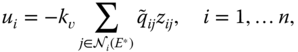
‐ and ![]() ‐direction components of the control inputs
‐direction components of the control inputs ![]() ,
, ![]() are given in Figure 2.7.
are given in Figure 2.7.

Figure 2.5Formation acquisition: agent trajectories  ,
,  .
.

Figure 2.6Formation acquisition: distance errors  ,
,  .
.

Figure 2.7Formation acquisition: control inputs  ,
,  .
.
A second simulation was conducted to illustrate the local nature of the stability result, as discussed in Section 2.1. To this end, the distance between each agent at ![]() and its corresponding target position was increased by selecting the initial conditions according to 2.76 with
and its corresponding target position was increased by selecting the initial conditions according to 2.76 with ![]() . The simulation results in Figure 2.8 show the agents reaching an incorrect formation due to
. The simulation results in Figure 2.8 show the agents reaching an incorrect formation due to ![]() . Notice that this incorrect formation corresponds to a flip ambiguity where edges 4 and 7 are flipped over edge 3 (see labels in Figure 2.4). That is, in this case, the control drives the agents to a formation with guaranteed desired inter‐agent distances only for agent pairs
. Notice that this incorrect formation corresponds to a flip ambiguity where edges 4 and 7 are flipped over edge 3 (see labels in Figure 2.4). That is, in this case, the control drives the agents to a formation with guaranteed desired inter‐agent distances only for agent pairs ![]() since the agents are initially positioned such that dist
since the agents are initially positioned such that dist![]() dist
dist![]() . This is clear from the plots in Figure 2.9 where the distance errors have been segregated by whether
. This is clear from the plots in Figure 2.9 where the distance errors have been segregated by whether ![]() (subplot (a)) or
(subplot (a)) or ![]() (subplot (b)). One can see that all
(subplot (b)). One can see that all ![]() with
with ![]() converge to zero, but the
converge to zero, but the ![]() values that are not in the edge set 2.75 do not necessarily converge to zero.
values that are not in the edge set 2.75 do not necessarily converge to zero.

Figure 2.8Formation acquisition: agents converging to an ambiguous framework.

Figure 2.9Formation acquisition: (a) distance errors  ,
,  and (b) distance errors
  ,
,  .
.
Figure 2.8 indicates that agent 5 is the one that is not properly initialized and therefore causing convergence to the incorrect formation. Now consider that we modify the edge set of the framework in Figure 2.4 to
leading to the framework in Figure 2.10. Notice that agent 5 is now connected to agent 2, ensuring that this distance is directly controlled. If the simulation is re‐run with the exact same initial conditions as Figure 2.8, the agents will converge to the desired formation (up to rotation and translation), as shown in Figure 2.11. This suggests that, in practice, the edges of the desired framework should be judiciously chosen based on the actual formation at ![]() to avoid convergence to an ambiguous framework.
to avoid convergence to an ambiguous framework.

Figure 2.10Desired formation  with modified edge set.

Figure 2.11Formation acquisition: agents converging to correct formation after change in edge set.
2.6.2 Formation Maneuvering
The purpose here was to simulate the use of the control law given by 2.23, 2.15, and 2.24 to achieve (1.26) and (1.28). Two simulations were conducted: one in 2D and the other in 3D.
Simulation 1: In this simulation, the agents were required to form a regular convex pentagon on the plane while maneuvering according to 2.24 with
The desired formation ![]() is shown in Figure 2.12. The five outer vertices of the pentagon represent the followers while the vertex at the geometric center of the pentagon represents the leader about which the followers will rotate. Thus, here,
is shown in Figure 2.12. The five outer vertices of the pentagon represent the followers while the vertex at the geometric center of the pentagon represents the leader about which the followers will rotate. Thus, here, ![]() . The desired framework was made minimally rigid and infinitesimally rigid by introducing 9 (
. The desired framework was made minimally rigid and infinitesimally rigid by introducing 9 (![]() ) edges with all followers connected to the leader. The edge set was selected as
) edges with all followers connected to the leader. The edge set was selected as
The desired inter‐agent distances were ![]() and
and ![]() .
.

Figure 2.12Formation maneuvering (Simulation 1): desired formation  .
.
The initial conditions of the agents were selected by 2.76 with ![]() and
and ![]() , while the control gain
, while the control gain ![]() was set to 1.
was set to 1.
Figure 2.13 shows snapshots of the actual formation ![]() over time, where the dotted line represents the leader trajectory. Notice that by
over time, where the dotted line represents the leader trajectory. Notice that by ![]() , the agents have virtually formed the desired shape while simultaneously translating and rotating according to 2.77. The rotation is counterclockwise about the axis coming out of the page based on the right‐hand rule. All the distance errors
, the agents have virtually formed the desired shape while simultaneously translating and rotating according to 2.77. The rotation is counterclockwise about the axis coming out of the page based on the right‐hand rule. All the distance errors ![]() ,
, ![]() are depicted in Figure 2.14 and converge to zero as expected. The
are depicted in Figure 2.14 and converge to zero as expected. The ![]() ‐ and
‐ and ![]() ‐direction components of the control inputs
‐direction components of the control inputs ![]() ,
, ![]() are given in Figure 2.15. Notice that in the
are given in Figure 2.15. Notice that in the ![]() (resp.,
(resp., ![]() ) direction, the control input converges to the first (resp., second) element of
) direction, the control input converges to the first (resp., second) element of ![]() in 2.77 plus the contribution from the angular velocity (see 2.24).
in 2.77 plus the contribution from the angular velocity (see 2.24).

Figure 2.13Formation maneuvering (Simulation 1): snapshots of  at different instants of time.

Figure 2.14Formation maneuvering (Simulation 1): distance errors  ,
,  .
.

Figure 2.15Formation maneuvering (Simulation 1): control inputs  ,
,  .
.
Simulation 2: Here, the desired formation was selected to be a cube with edge length of 2 as shown in Figure 2.16. For ease of implementation, the eight vertices of the cube were chosen to represent the followers while the geometric center of the cube (point ![]() was chosen to represent the leader (i.e., agent 9), thus
was chosen to represent the leader (i.e., agent 9), thus ![]() . The required minimally rigid and infinitesimally rigid conditions of
. The required minimally rigid and infinitesimally rigid conditions of ![]() were enforced by introducing 21 (
were enforced by introducing 21 (![]() ) edges with all followers connected to the leader. The edge set was set to
) edges with all followers connected to the leader. The edge set was set to

The desired inter‐agent distances were given by ![]() ,
, ![]()
![]()
![]()
![]()
![]() , and
, and ![]() . The initial conditions were chosen as in Simulation 1.
. The initial conditions were chosen as in Simulation 1.

Figure 2.16Formation maneuvering (Simulation 2): desired formation  .
.
The maneuvering velocity was set to
which corresponds to a circular orbit of the formation about the ![]() ‐axis with the same side of the cube always facing the interior of the orbit. The control gain was again chosen as 1. Figure 2.17 shows snapshots of the formation maneuver, the distance errors are shown in Figure 2.18, and the control inputs are shown in Figure 2.19.
‐axis with the same side of the cube always facing the interior of the orbit. The control gain was again chosen as 1. Figure 2.17 shows snapshots of the formation maneuver, the distance errors are shown in Figure 2.18, and the control inputs are shown in Figure 2.19.

Figure 2.17Formation maneuvering (Simulation 2): snapshots in time of the formation maneuver. The asterisk denotes the orbit center, the dots are the leader trajectory, the squares are the agent 2 trajectory, and the crosses are the agent 8 trajectory.

Figure 2.18Formation maneuvering (Simulation 2): distance errors  ,
,  .
.
Figure 2.19Formation maneuvering (Simulation 2): control inputs  ,
,  in the
  ,
,  , and
, and  directions.
2.6.3 Flocking
The flocking schemes from Section 2.3 were simulated for the case where five agents have to acquire the desired formation shown in Figure 2.4 and flock with some desired velocity. The control and observer gains in (2.28) and 2.36 were set to ![]() and
and ![]() , respectively. The initial positions of the agents were randomly generated by 2.76 with
, respectively. The initial positions of the agents were randomly generated by 2.76 with ![]() while
while ![]() .
.
First, the controller–observer scheme in (2.28) was simulated with desired velocity ![]() under two conditions: one where only agent 2 has knowledge of
under two conditions: one where only agent 2 has knowledge of ![]() (
(![]() ) and the other where
) and the other where ![]() . The trajectory of the actual formation
. The trajectory of the actual formation ![]() is shown in Figure 2.20 for the case where
is shown in Figure 2.20 for the case where ![]() . The inter‐agent distances errors and velocity estimation errors are shown Figures 2.21 and 2.22, respectively. The control inputs are given in Figure 2.23. As can be seen from the figures, the agents meet the flocking objective by approximately
. The inter‐agent distances errors and velocity estimation errors are shown Figures 2.21 and 2.22, respectively. The control inputs are given in Figure 2.23. As can be seen from the figures, the agents meet the flocking objective by approximately ![]() . Notice from Figure 2.22 that the estimation error with the fastest convergence is
. Notice from Figure 2.22 that the estimation error with the fastest convergence is ![]() since agent 2 has direct access to
since agent 2 has direct access to ![]() . This is followed by
. This is followed by ![]() and
and ![]() , which are directly connected to agent 2 (see Figure 2.4), and then
, which are directly connected to agent 2 (see Figure 2.4), and then ![]() and
and ![]() , which are one hop away from agent 2.
, which are one hop away from agent 2.

Figure 2.20Flocking (continuous controller–observer;  ): snapshots of
  at different instants of time.

Figure 2.21Flocking (continuous controller–observer;  ): distance errors
  ,
,  .
.

Figure 2.22Flocking (continuous controller–observer;  ): velocity estimation errors
  ,
,  in the
  and
and  directions.

Figure 2.23Flocking (continuous controller–observer;  ): control inputs
  ,
,  in the
  and
and  directions.
The results for the case where ![]() are given in Figures 2.24–2.26. One can see from Figure 2.25 that the estimation errors of all agents converge faster than in Figure 2.22 since the flocking velocity is available to more agents, resulting in faster consensus. This is also reflected in the distance errors, which also have a faster convergence.
are given in Figures 2.24–2.26. One can see from Figure 2.25 that the estimation errors of all agents converge faster than in Figure 2.22 since the flocking velocity is available to more agents, resulting in faster consensus. This is also reflected in the distance errors, which also have a faster convergence.

Figure 2.24Flocking (continuous controller–observer;  ): distance errors
  ,
,  .
.

Figure 2.25Flocking (continuous controller–observer;  ): velocity estimation errors
  ,
,  in the
  and
and  directions.

Figure 2.26Flocking (continuous controller–observer;  ): control inputs
  ,
,  in the
  and
and  directions.
Next, the controller–observer in (2.28) was simulated with desired velocity ![]() and
and ![]() . Due to the inability of observer ( 2.28b
) in ensuring
. Due to the inability of observer ( 2.28b
) in ensuring ![]() as
as ![]() when
when ![]() is time varying, one can see from Figure 2.27 that the flocking velocity estimation error in the
is time varying, one can see from Figure 2.27 that the flocking velocity estimation error in the ![]() direction is nonzero. This also affects the formation acquisition as evidenced by the inter‐agent distances errors in Figure 2.28.
direction is nonzero. This also affects the formation acquisition as evidenced by the inter‐agent distances errors in Figure 2.28.

Figure 2.27Flocking (continuous controller–observer;  ): velocity estimation errors with time‐varying desired velocity.

Figure 2.28Flocking (continuous controller–observer;  ): distance errors with time‐varying desired velocity.
When the discontinuous controller–observer (2.28a) and 2.36 is applied to the same time‐varying velocity case, we get the results shown in Figures 2.29–2.31. The variable structure nature of the observer allows for a fast estimation of the flocking velocity, which in turn causes the agent velocities to converge to ![]() by
by ![]() .
.

Figure 2.29Flocking (discontinuous controller–observer;  ): distance errors with time‐varying desired velocity.

Figure 2.30Figure 2.30Flocking (discontinuous controller–observer;  ): velocity estimation errors with time‐varying desired velocity.
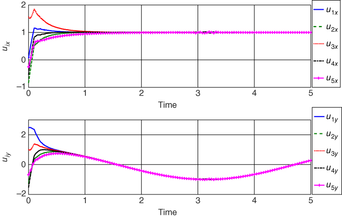
Figure 2.31Flocking (discontinuous controller–observer;  ): control inputs.
2.6.4 Target Interception
In this simulation, we tested the control law defined by 2.53, 2.54, and 2.45 in satisfying (1.26) and (1.29). The unknown velocity of the moving target was set to
with initial position ![]() . We used the same desired formation topology defined in Section 2.6.2 (see Figure 2.12) with agent 6 being the leader that is responsible for tracking the target. The initial conditions were again set by 2.76 with
. We used the same desired formation topology defined in Section 2.6.2 (see Figure 2.12) with agent 6 being the leader that is responsible for tracking the target. The initial conditions were again set by 2.76 with ![]() and
and ![]() while
while ![]() . The control gains were set to
. The control gains were set to ![]() ,
, ![]() , and
, and ![]() . The fact that this value for
. The fact that this value for ![]() does not satisfy 2.47 since
does not satisfy 2.47 since ![]() from 2.80 will demonstrate that this condition is indeed only sufficient for stability of the target tracking error.
from 2.80 will demonstrate that this condition is indeed only sufficient for stability of the target tracking error.
Figure 2.32 shows the leader intercepting the target and the followers simultaneously enclosing it with the pentagon formation. The inter‐agent distance errors are given in Figure 2.33. Figure 2.34 displays the control inputs of each agent converging to ![]() (viz., 1 in the
(viz., 1 in the ![]() direction and
direction and ![]() in the
in the ![]() direction), despite the target velocity being unknown.
direction), despite the target velocity being unknown.

Figure 2.32Target interception: snapshots of  at different instants of time along with target motion.

Figure 2.33Target interception: distance errors  ,
,  .
.

Figure 2.34Target interception: control inputs  ,
,  .
.
2.6.5 Dynamic Formation
We simulated a scenario where the formation needs to vary in order to move through a narrow passageway. To this end, control law 2.73 was simulated since it includes the dynamic formation acquisition control law 2.71. The primary objective here is 2.66.
The desired dynamic formation ![]() was set to a regular convex pentagon that expanded and contracted uniformly over time.8 The desired formation at
was set to a regular convex pentagon that expanded and contracted uniformly over time.8 The desired formation at ![]() ,
, ![]() , is the same one used in the simulation of Section 2.6.1 and depicted in Figure 2.4. The desired formation was made dynamic by setting the vertex coordinates to
, is the same one used in the simulation of Section 2.6.1 and depicted in Figure 2.4. The desired formation was made dynamic by setting the vertex coordinates to

where 2.74 was used and
As a result, the desired inter‐agent distances were given by

The desired swarm velocity was set to ![]() . The initial conditions of the agents were selected by 2.76 with
. The initial conditions of the agents were selected by 2.76 with ![]() and
and ![]() . The control gain
. The control gain ![]() was set to 10.
was set to 10.
Figure 2.35 shows the agent trajectories over time as they track the desired formation while translating according to ![]() . The effective tracking of
. The effective tracking of ![]() is better depicted by Figure 2.36, which shows the inter‐agent distance errors approaching zero. The
is better depicted by Figure 2.36, which shows the inter‐agent distance errors approaching zero. The ![]() ‐ and
‐ and ![]() ‐direction components of the control inputs are given in Figure 2.37, where the left plots show their transient behavior (
‐direction components of the control inputs are given in Figure 2.37, where the left plots show their transient behavior (![]() ) and the right plots show the steady‐state behavior (
) and the right plots show the steady‐state behavior (![]() ).
).

Figure 2.35Dynamic formation: snapshots of  at different instants of time along with agent trajectories.

Figure 2.36Dynamic formation: distance errors  ,
,  .
.

Figure 2.37Dynamic formation: control inputs 
 .
.
2.7 Notes and References
Several results on formation control of multi‐agent systems based on the single‐integrator model that consider the stabilization of the inter‐agent distance dynamics to desired distances have appeared in the literature. The first to use the gradient descent control law for the 2D formation acquisition problem were 23,46. A similar 2D formation acquisition controllers was discussed in 47, whereas 3D formations were considered in 48. In 49, the authors provided a unified approach for the exponential stability analysis of minimally and nonminimally rigid formations. In 50,51, 2D formation maneuvering controllers were introduced that only considered swarm translation. 2D formation maneuvering (translation only) and target interception schemes were designed in 2. In 52, the 2D translational maneuvering scheme involved a leader with a constant velocity command and followers who track the leader while maintaining the formation shape. The control law consisted of the standard gradient descent formation acquisition term plus an integral term to ensure zero steady‐state error with respect to the velocity command. In all the above results, the desired formation is assumed static. A related problem is when the control objective is the stabilization to a static formation with a desired orientation. This problem was recently addressed in 53, where the controller included a term to perform orientation stabilization in addition to the gradient descent formation acquisition control. A minimal number of agents should have knowledge of a global coordinate system for this to occur. For other work that addresses this problem, see 53. Recently, an interesting approach for ensuring convergence to a unique formation (i.e., without ambiguities) was proposed in 54 where the desired formation is defined with both distance and signed area constraints.
To the best of our knowledge, the Lyapunov function candidate ( 2.10
) first appeared in 55, where it was used in the stability analysis of triangular formations. The local nature of our stability results in Euclidean space is inherent to the formation control approach based on rigid graph theory; see, e.g., 23,46,47,56,57. Even in the case of three agents attempting to form a triangle, the stability set excludes the situation where the agents are initially collocated or collinear. In fact, the invariance of the collinear set appears to have been first shown in 23. For ![]() ‐agent formations, the size of the stability set likely decreases with increasing
‐agent formations, the size of the stability set likely decreases with increasing ![]() since the number of possible framework ambiguities grows. The condition on the initial distance error given in the theorems of this chapter is a sufficient condition for stability, and simply indicates that a stability set exists. In practice, the stability set is best quantified by running simulations for different initial conditions since its size is likely larger than that provided by the sufficient condition.
since the number of possible framework ambiguities grows. The condition on the initial distance error given in the theorems of this chapter is a sufficient condition for stability, and simply indicates that a stability set exists. In practice, the stability set is best quantified by running simulations for different initial conditions since its size is likely larger than that provided by the sufficient condition.
The directionality of the information exchange among agents is an important design factor. This issue is of practical importance since it relates to the number of communication, sensing, and/or control channels of the multi‐agent system. In the case of bidirectional information exchange, a pair of agents concurrently controls the distance between them, whereas only one agent in the pair is responsible for this task in the unidirectional case. In terms of graph theory, bidirectional (resp., unidirectional) formation controllers are based on undirected (resp., directed) graphs. Undirected formation controllers have built‐in redundancy, providing robustness. However, it can also lead to instability in the formation acquisition if agent pairs use slightly different values for the distance between them due to measurement errors 31. In 58, 59 it was shown that this measurement mismatch causes a distortion of the formation from its desired shape and a circular (resp., helical) orbit of the distorted formation in 2D (resp., 3D). One possible remedy for this problem is to have the agents communicate their respective measurements to one another and then use a common value for control (e.g., the average of the two measurements). A more rigorous solution was proposed in 60 by using an estimator‐based gradient control law to make the system robust against measurement inconsistency. Yet another solution is to use a directed graph‐based controller since it reduces the overall number of communication/sensing/control channels while avoiding the potential conflict between a pair of agents trying to achieve the same objective. However, in directed graphs it is possible to have cycles in the pathways, which are more challenging to control and can lead to formation instability 57. Therefore, the issue of cyclic versus acyclic graphs is an important consideration for directed formation control.
While the results in this book use undirected graphs, the directed graph problem has also received considerable attention. The idea of applying input‐to‐state stability to study the stability properties of directed acyclic formation graphs was discussed in 61, but without considering the control design problem. For directed graphs, the traditional notion of rigidity is not enough to maintain the formation structure. In 31, the concept of rigidity of a directed graph was first discussed and a formation control law was proposed that assumes the global position of the leader and first‐follower agents are known in a 2D acyclic graph. A method for analyzing the rigidity of 2D directed formations that have a leader–follower structure was provided in 62 without consideration of the control design problem. The concept of rigidity of a directed graph was refined and formalized in 63,64 by introducing the notions of constraint consistence and persistence. The intuitive meaning of a constraint consistent graph is that every agent is able to satisfy all its distance constraints when all the others are trying to do the same. A directed graph that is both rigid and constraint consistent is called persistent The notion of persistence was introduced in 63 for 2D graphs and generalized to higher dimensional graphs in 64. The problem of a triangular formation with cyclic ordering was considered in 65 and a locally exponentially stabilizing control law was proposed based on measurements of all inter‐agent distances but only one inter‐agent angle. A generalized control law for cyclic triangular formations was presented in 66. In 7, a control law was designed for directed planar formations of ![]() agents modeled by a minimally persistent graph with a leader‐first‐follower topology. A controller for
agents modeled by a minimally persistent graph with a leader‐first‐follower topology. A controller for ![]() ‐agent persistent formations whose graph is constructed by a sequence of Henneberg insertions was proposed in 23, and the local asymptotic stability of the desired formation was proven using the linearized dynamics. The stability of the control from 23 was analyzed in 55 using differential geometry for a three‐agent cyclic formation. In 57, the result from 7 was generalized to also include minimally persistent graphs with leader‐remote‐follower and coleader topologies, which are inherently cyclic. In 67, a discontinuous controller was proposed to achieve finite‐time convergence to the desired formation for acyclic persistent graphs.
‐agent persistent formations whose graph is constructed by a sequence of Henneberg insertions was proposed in 23, and the local asymptotic stability of the desired formation was proven using the linearized dynamics. The stability of the control from 23 was analyzed in 55 using differential geometry for a three‐agent cyclic formation. In 57, the result from 7 was generalized to also include minimally persistent graphs with leader‐remote‐follower and coleader topologies, which are inherently cyclic. In 67, a discontinuous controller was proposed to achieve finite‐time convergence to the desired formation for acyclic persistent graphs.
While the above discussion was focused on formation control approaches based on rigid graph theory and controlling inter‐agent distances, other approaches can be found in the literature. The treatment of multi‐agent formations as a consensus control problem was discussed in 39 where the information state, whose value is to be negotiated by the consensus algorithm, is the center of the formation. A broad literature review of different formation control schemes is presented in Section of 4. In 2, formation acquisition controllers were designed using the gradient of a general potential function that represents the repulsion/attraction between agents and is chosen based on the desired inter‐agent distances. Formation maneuvering and target interception schemes were also designed in 2 by adding appropriate terms to the gradient law. Formation acquisition (static and dynamic) and formation maneuvering protocols were introduced in 68 that ensure convergence to the desired formation in finite time. A complex graph Laplacian scheme is presented in 69 for the formation acquisition problem where the formation scale is determined by two leader agents. The idea of triangular formation acquisition using only inter‐agent angle measurements was proposed in 70. In 56, a formation control strategy was demonstrated that is based on the distributed estimation of the agent absolute positions from relative position measurements when the inter‐agent sensing/communication graph has a spanning tree.
Relatively few results exist for the general formation maneuvering (translation and rotation) problem. A 3D formation maneuvering control law was presented in 71 but without considering the stability of the formation acquisition. In 72 a controller was proposed that can steer the entire formation in rotation and/or translation in 3D. The rotation component was specified relative to a body‐fixed frame whose origin is at the centroid of the desired formation and needs to be known.
The material in this chapter is mostly based on the work in 73–75. The observers used in the flocking problem of Section 2.3 are based on 76, 77.