9
Predictive Analysis to Support Fog Application Deployment
Antonio Brogi Stefano Forti and Ahmad Ibrahim
9.1 Introduction
Connected devices are changing the way we live and work. In the next years, the Internet of Things (IoT) is expected to bring more and more intelligence around us, being embedded in or interacting with the objects that we will use daily. Self‐driving cars, autonomous domotics systems, energy production plants, agricultural lands, supermarkets, healthcare, and embedded AI will more and more exploit devices and things that are an integral part of the Internet and of our existence without us being aware of them. CISCO foresees 50 billion connected entities (people, machines, and connected things) by 2020 [1], and estimates they will have generated around 600 zettabytes of information by that time, only 10% of which will be useful to some purpose [2]. Furthermore, cloud connection latencies are not adequate to host real‐time tasks such as life‐saving connected devices, augmented reality, or gaming [3]. In such a perspective, the need to provide processing power, storage, and networking capabilities to run IoT applications closer to sensors and actuators has been highlighted by various authors, such as [4, 5].
Fog computing [6] aims at selectively pushing computation closer to where data are produced, by exploiting a geographically distributed multitude of heterogeneous devices (e.g., gateways, micro‐datacenters, embedded servers, personal devices) spanning the continuum from cloud to things. On one hand, this will enable low‐latency responses to (and analysis of) sensed events, on the other hand, it will relax the need for (high) bandwidth availability from/to the cloud [7]. Overall, fog computing is expected to fruitfully extend the IoT+Cloud scenario, enabling quality‐of‐service‐ (QoS) and context‐aware application deployments [5].
Modern applications usually consist of many independently deployable components – each with its hardware, software, and IoT requirements – that interact together distributedly. Such interactions may have stringent QoS requirements – typically on latency and bandwidth – to be fulfilled for the deployed application to work as expected [3]. If some application components (i.e., functionalities) are naturally suited to the cloud (e.g., service back‐ends) and others are naturally suited to edge devices (e.g., industrial control loops), there are some applications for which functionality segmentation is not as straightforward (e.g., short‐ to medium‐term analytics). Supporting deployment decision in the fog also requires comparing a multitude of offerings where providers can deploy applications to their infrastructure integrated with the cloud, with the IoT, with federated fog devices as well as with user‐managed devices. Moreover, determining deployments of a multi‐component application to a given fog infrastructure, while satisfying its functional and nonfunctional constraints, is an NP‐hard problem [8].
As highlighted in [9], novel fog architectures call for modeling complex applications and infrastructures, based on accurate models of application deployment and behavior to predict their runtime performance, also relying on historical data [10]. Algorithms and methodologies are to be devised to help deciding how to map each application functionality (i.e., component) to a substrate of heterogeneously capable and variably available nodes [11].
All of this, including node mobility management, and taking into account possible variations in the QoS of communication links (fluctuating bandwidth, latency, and jitter over time) supporting component–component interactions as well as the possibility for deployed components to remotely interact with the IoT via proper interfaces [10]. Moreover, other orthogonal constraints such as QoS‐assurance, operational cost targets, and administration or security policies should be considered when selecting candidate deployments.
Clearly, manually determining fog applications (re‐)deployments is a time‐consuming, error‐prone, and costly operation, and deciding which deployments may perform better – without enacting them – is difficult. Modern enterprise IT is eager for tools that permit to virtually compare business scenarios and to design both pricing schemes and SLAs by exploiting what‐if analyses [12] and predictive methodologies, abstracting unnecessary details.
In this chapter, we present an extended version of FogTorchΠ [13, 14], a prototype based on a model of the IoT+Fog+Cloud scenario to support application deployment in the Fog. FogTorchΠ permits to express processing capabilities, QoS attributes (viz., latency and bandwidth) and operational costs (i.e., costs of virtual instances, sensed data) of a fog infrastructure, along with processing and QoS requirements of an application. In short, FogTorchΠ:
- Determines the deployments of an application over a fog infrastructure that meet all application (processing, IoT and QoS) requirements.
- Predicts the QoS‐assurance of such deployments against variations in the latency and bandwidth of communications links.
- Returns an estimate of the fog resource consumption and a monthly cost of each deployment.
Overall, the current version of FogTorchΠ features (i) QoS‐awareness to achieve latency reduction, bandwidth savings and to enforce business policies, (ii) context‐awareness to suitably exploit both local and remote resources, and (iii) cost‐awareness to determine the most cost‐effective deployments among the eligible ones.
FogTorchΠ models the QoS of communication links by using probability distributions (based on historical data), describing variations in featured latency or bandwidth over time, depending on network conditions. To handle input probability distributions and to estimate the QoS assurance of different deployments, FogTorchΠ exploits the Monte Carlo method [17]. FogTorchΠ also exploits a novel cost model that extends existing pricing schemes for the cloud to fog computing scenarios, whilst introducing the possibility of integrating such schemes with financial costs that originate from the exploitation of IoT devices (sensing‐as‐a‐service [15] subscriptions or data transfer costs) in the deployment of applications. We show and discuss how predictive tools like FogTorchΠ can help IT experts in deciding how to distribute application components over fog infrastructures in a QoS‐ and context‐aware manner, also considering cost of fog application deployments.
The rest of this chapter is organized as follows. After introducing a motivating example of a smart building application (Section ), we describe FogTorchΠ predictive models and algorithms (Section ). Then, we present and discuss the results obtained by applying FogTorchΠ to the motivating example (Section ). Afterward, some related work and a comparison with the iFogSim simulator are provided (Section ). Finally, we highlight future research directions (Section ) and draw some concluding remarks (Section ).
9.2 Motivating Example: Smart Building
Consider a simple fog application (Figure 9.1) that manages fire alarm, heating and air conditioning systems, interior lighting, and security cameras of a smart building. The application consists of three microservices:
- IoTController, interacting with the connected cyber‐physical systems,
- DataStorage, storing all sensed information for future use and employing machine learning techniques to update sense‐act rules of the IoTController so to optimize heating and lighting management based on previous experience and/or on people behavior, and
- Dashboard, aggregating and visualizing collected data and videos, as well as allowing users to interact with the system.

Figure 9.1 Fog application of the motivating example.1
Each microservice 1 represents an independently deployable component of the application [16] and has hardware and software requirements in order to function properly (as indicated in the gray boxes associated with components in Figure 9.1). Hardware requirements are expressed in terms of the virtual machine (VM) types 2 listed in Table 9.1 and must be fulfilled by the VM that will host the deployed component.
Table 9.1 Hardware specification for different VM types.
| VM Type | vCPUs | RAM (GB) | HDD (GB) |
| tiny | 1 | 1 | 10 |
| small | 1 | 2 | 20 |
| medium | 2 | 4 | 40 |
| large | 4 | 8 | 80 |
| xlarge | 8 | 16 | 160 |
Application components must cooperate so that well‐defined levels of service are met by the application. Hence, communication links supporting component‐component interactions should provide suitable end‐to‐end latency and bandwidth (e.g., the IoTController should reach the DataStorage within 160 ms and have at least 0.5 Mbps download and 3.5 Mbps upload free bandwidths). Component–things interactions have similar constraints, and also specify the sampling rates at which the IoTController is expected to query things at runtime (e.g., the IoTController should reach a fire_sensor, queried once per minute, within 100 ms having at least 0.1 Mbps download and 0.5 Mbps upload free bandwidths).
Figure 9.2 shows the infrastructure – two cloud data centers, three fog nodes, and nine things – selected by the system integrators in charge of deploying the smart building application for one of their customers. The deployed application will have to exploit all the things connected to Fog 1 and the weather_station_3 at Fog 3. Furthermore, the customer owns Fog 2, what makes deploying components to that node cost‐free.
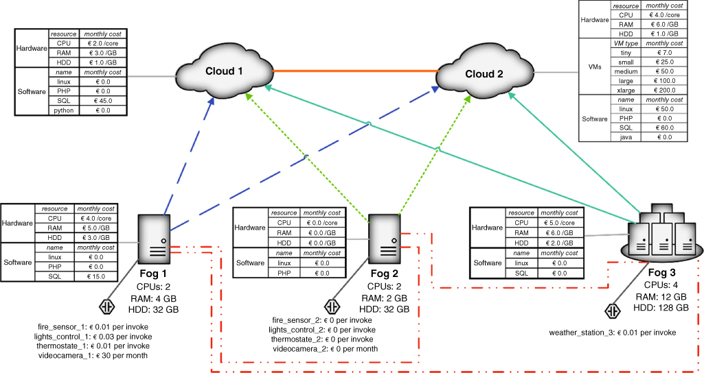
Figure 9.2 Fog infrastructure of the motivating example.4
All fog and cloud nodes are associated with pricing schemes, either to lease an instance of a certain VM type (e.g., a tiny instance at Cloud 2 costs €7 per month), or to build on‐demand instances by selecting the required number of cores and the needed amount of RAM and HDD to support a given component.
Fog nodes offer software capabilities, along with consumable (i.e., RAM, HDD) and non-consumable (i.e., CPUs) hardware resources. Similarly, cloud nodes offer software capabilities, while cloud hardware is considered unbounded, assuming that, when needed, one can always purchase extra instances.
Finally, Table 9.2 lists the QoS of the end‐to‐end communication links supported by the infrastructure of Figure 9.2, connecting fog and cloud nodes. They are represented as probability distributions based on real data 4 , to account for variations in the QoS they provide. Mobile communication links at Fog 2 initially feature a 3G Internet access. As per the current technical proposals (e.g., [6] and [10]), we assume fog and cloud nodes are able to access directly connected things as well as things at neighboring nodes via a specific middleware layer (through the associated communication links).
Table 9.2 QoS profiles associated to the communication links.
| Dash Type | Profile | Latency | Download | Upload |
|
|
Satellite 14M | 40 ms |
98%: 10.5 Mbps 2%: 0 Mbps |
98%: 4.5 Mbps 2%: 0 Mbps |
|
|
3G | 54 ms |
99.6%: 9.61 Mbps 0.4%: 0 Mbps |
99.6%: 2.89 Mbps 0.4%: 0 Mbps |
| 4G | 53 ms |
99.3%: 22.67 Mbps 0.7%: 0 Mbps |
99.4%: 16.97 Mbps 0.6%: 0 Mbps |
|
|
|
VDSL | 60 ms | 60 Mbps | 6 Mbps |
|
|
Fiber | 5 ms | 1000 Mbps | 1000 Mbps |
|
|
WLAN | 15 ms |
90%: 32 Mbps 10%: 16 Mbps |
90%: 32 Mbps 10%: 16 Mbps |
Planning to sell the deployed solution for €1,500 a month, the system integrators set the limit of the monthly deployment cost at €850. Also, the customer requires the application to be compliant with the specified QoS requirements at least 98% of the time. Then, interesting questions for the system integrators before the first deployment of the application are, for instance:
- Q1(a) — Is there any eligible deployment of the application reaching all the needed things at Fog 1 and Fog 3, and meeting the aforementioned financial (at most € 850 per month) and QoS‐assurance (at least 98% of the time) constraints? 3
- Q1(b) — Which eligible deployments minimize resource consumption in the fog layer so to permit future deployment of services and sales of virtual instances to other customers?
Suppose also that with an extra monthly investment of €20, system integrators can exploit a 4G connection at Fog 2. Then:
- Q2 — Would there be any deployment that complies with all previous requirements and reduces financial cost and/or consumed fog resources if upgrading from 3G to 4G at Fog 2?
In Section , we will show how FogTorchΠ can be exploited to obtain answers to all the above questions.
9.3 Predictive Analysis with FogTorchΠ
9.3.1 Modeling Applications and Infrastructures
FogTorchΠ [13, 14] is an open‐source Java prototype 5 (based on the model presented in [8]) that determines eligible QoS‐, context‐ and cost‐aware multi‐component application deployments to fog infrastructures.
FogTorchΠ input consists of the following:
- Infrastructure I . The input includes a description of an infrastructure I specifying the IoT devices, the fog nodes, and the cloud data centers available for application deployment (each with its hardware and software capabilities), along with the probability distributions of the QoS (viz., latency, bandwidth) featured by the available (cloud‐to‐fog, fog‐to‐fog and fog‐to‐things) end‐to‐end communication links 6 and cost for purchasing sensed data and for cloud/fog virtual instances.
- Multicomponent application A . This specifies all hardware (e.g., CPU, RAM, storage), software (e.g., OS, libraries, frameworks) and IoT requirements (e.g., which type of things to exploit) of each component of the application, and the QoS (i.e., latency and bandwidth) needed to adequately support component–component and component–thing interactions once the application has been deployed.
- Things binding ϑ . This maps each IoT requirement of an application component to an actual thing available in I .
- Deployment policy δ . The deployment policy white‐lists the nodes where A components can be deployed 7 according to security or business‐related constraints.

Figure 9.3 Bird's‐eye view of FogTorchΠ.
Figure 9.3 offers a bird's‐eye view of FogTorchΠ, with the input to the tool on the left‐hand side and its output on the right‐hand side. In the next sections we will present the backtracking search exploited by FogTorchΠ to determine the eligible deployments, the models used to estimate the fog resource consumption and cost of such deployments, and the Monte Carlo method [17] employed to assess their QoS‐assurance against variations in the latency and bandwidth featured by communication links.
9.3.2 Searching for Eligible Deployments
Based on the input described in Section , FogTorchΠ determines all the eligible deployments of the components of an application A to cloud or fog nodes in an infrastructure I .
An eligible deployment Δ maps each component γ of A to a cloud or fog node n in I so that:
- n complies with the specified deployment policy δ (viz., n ∈ δ(γ)) and it satisfies the hardware and software requirements of γ,
- The things specified in the Things binding ϑ are all reachable from node n (either directly or through a remote end‐to‐end link),
- The hardware resources of n are enough to deploy all components of A mapped to n, and
- The component–component and component–thing interactions QoS requirements (on latency and bandwidth) are all satisfied.
To determine the eligible deployments of a given application A to a given infrastructure I (complying with both ϑ and δ ), FogTorchΠ exploits a backtracking search, as illustrated in the algorithm of Figure 9.4. The preprocessing step (line 2) builds, for each software component γ∈ A , the dictionary K[γ] of fog and cloud nodes that satisfy conditions (1) and (2) for a deployment to be eligible, and also meet the latency requirements for the things requirements of component γ. If there exists even one component for which K[γ] is empty, the algorithm immediately returns an empty set of deployments (lines 3–5). Overall, the preprocessing completes in O(N) time, with N being the number of available cloud and fog nodes, having to check the capabilities of at most all fog and cloud nodes for each application component.

Figure 9.4 Pseudocode of the exhaustive search algorithm.
The call to the BACKTRACKSEARCH( D, Δ, A, I, K, ϑ ) procedure (line 7) inputs the result of the preprocessing and looks for eligible deployments. It visits a (finite) search space tree having at most N nodes at each level and height equal to the number Γ of components of A . As sketched in Figure 9.5, each node in the search space represents a (partial) deployment Δ, where the number of deployed components corresponds to the level of the node. The root corresponds to an empty deployment, nodes at level i are partial deployments of i components, and leaves at level Γ contain complete eligible deployments. Edges from one node to another represent the action of deploying a component to some fog or cloud node. Thus, search completes in O(N Γ) time.

Figure 9.5 Search space to find eligible deployments of A to I .
At each recursive call, BACKTRACKSEARCH (D, Δ, A, I, K, ϑ) first checks whether all components of A have been deployed by the currently attempted deployment and, if so, it adds the found deployment to set D (lines 2–3) as listed in Figure 9.6, and returns to the caller (line 4). Otherwise, it selects a component still to be deployed (SELECTUNDEPLOYEDCOMPONENT (Δ, A)) and it attempts to deploy it to a node chosen in K[γ] (SELECTDEPLOYMENTNODE (K[γ], A). The ISELIGIBLE (Δ, γ, n, A, I, ϑ) procedure (line 8) checks conditions (3) and (4) for a deployment to be eligible and, when they hold, the DEPLOY (Δ, γ, n, A, I, ϑ) procedure (line 9) decreases the available hardware resources and bandwidths in the infrastructure, according to the new deployment association. UNDEPLOY (Δ, γ, n, I, A, ϑ) (line 11) performs the inverse operation of DEPLOY (Δ, γ, n, A, I, ϑ), releasing resources and freeing bandwidth when backtracking on a deployment association.

Figure 9.6 Pseudocode for the backtracking search.
9.3.3 Estimating Resource Consumption and Cost
Procedure FINDDEPLOYMENTS (A, I, δ, ϑ) computes an estimate of fog resource consumption and of the monthly cost 8 of each given deployment.
The fog resource consumption that is output by FogTorchΠ indicates the aggregated averaged percentage of consumed RAM and storage in the set of fog nodes 9 F , considering all deployed application components γ ∈ A . Overall, resource consumption is computed as the average

where RAM(γ), HDD(γ) indicate the amount of resources needed by component γ , and RAM(f), HDD(f ) are the total amount of such resources available at node f.
To compute the estimate of the monthly cost of deployment for application A to infrastructure I , we propose a novel cost model that extends to fog computing previous efforts in cloud cost modelling [18] and includes costs due to IoT [19], and software costs.
At any cloud or fog node n , our cost model considers that a hardware offering H can be either a default VM (Table 9.1) offered at a fixed monthly fee or an on‐demand VM (built with an arbitrary amount of cores, RAM and HDD). Being R the set of resources considered when building on‐demand VMs (viz., R = {CPU, RAM, HDD}), the estimated monthly cost for a hardware offering H at node n is:

where c(H, n) is the monthly cost of a default VM offering H at fog or cloud node n , while H. ρ indicates the amount of resources ρ ∈ R used by 10 the on‐demand VM represented by H , and c(ρ, n) is the unit monthly cost at n for resource ρ.
Analogously, for any given cloud or fog node n , a software offering S can be either a predetermined software bundle or an on‐demand subset of the software capabilities available at n (each sold separately). The estimated monthly cost for S at node n is:

where c(S, n) is the cost for the software bundle S at node n , and c(s, n) is the monthly cost of a single software s at n .
Finally, in sensing‐as‐a‐service [15] scenarios, a thing offering T exploiting an actual thing t can be offered at a monthly subscription fee or through a pay‐per‐invocation mechanism. Then, the cost of offering T at thing t is:

where c(T, t) is the monthly subscription fee for T at t , while T. k is the number of monthly invocations expected over t , and c(t) is the cost per invocation at t (including thing usage and/or data transfer costs).
Assume that Δ is an eligible deployment for an application
A
to an infrastructure
I
, as introduced in Section . In addition, let γ ∈ A
be a component of the considered application
A
, and let ![]() ,
, ![]() and
and ![]() be its hardware, software and things requirements, respectively. Overall, the expected monthly cost for a given deployment Δ can be first approximated by combining the previous pricing schemes as:
be its hardware, software and things requirements, respectively. Overall, the expected monthly cost for a given deployment Δ can be first approximated by combining the previous pricing schemes as:

Although the above formula provides an estimate of the monthly cost for a given deployment, it does not feature a way to select the “best” offering to match the application requirements at the VM, software and IoT levels. Particularly, it may lead the choice always to on‐demand and pay‐per‐invocation offerings when the application requirements do not match exactly default or bundled offerings, or when a cloud provider does not offer a particular VM type (e.g., starting its offerings from medium). This can lead to overestimating the monthly deployment cost.
For instance, consider the infrastructure of Figure 9.2 and the hardware requirements of a component to be deployed to Cloud 2, specified as R = {CPU : 1, RAM : 1GB, HDD : 20GB}. Since no exact matching exists between the requirements R and the offerings at Cloud 2, this first cost model would select an on‐demand instance, and estimate its cost of €30. 11 However, Cloud 2 also provides a small instance that can satisfy the requirements at a (lower) cost of €25.
Since larger VM types always satisfy smaller hardware requirements, bundled software offerings may satisfy multiple software requirements at a lower price, and subscription‐based thing offerings can be more or less convenient, depending on the number of invocations on a given thing, some policy must be used to choose the “best” offerings for each software, hardware and thing requirement of an application component. In what follows, we refine our cost model to also account for this.
A requirement‐to‐offering matching policy
p
m
(r, n) matches hardware or software requirements
r
of a component (![]() ) to the estimated monthly cost of the offering that will support them at cloud or fog node
n
, and a thing requirement
) to the estimated monthly cost of the offering that will support them at cloud or fog node
n
, and a thing requirement ![]() to the estimated monthly cost of the offering that will support
r
at thing
t
.
to the estimated monthly cost of the offering that will support
r
at thing
t
.
Overall, this refined version of the cost model permits an estimation of the monthly cost of Δ including a cost‐aware matching between application requirements and infrastructure offering (for hardware, software and IoT), chosen as per p m . Hence:

The current implementation of FogTorchΠ exploits a best‐fit lowest‐cost policy for choosing hardware, software and thing offerings. Indeed, it selects the cheapest between the first default VM (from tiny to xlarge) that can support ![]() at node
n
and the on‐demand offering built as per
at node
n
and the on‐demand offering built as per ![]() . Likewise, software requirements in
. Likewise, software requirements in ![]() are matched with the cheapest compatible version available at
n
, and thing per invocation offer is compared to monthly subscription so to select the cheapest.
12
are matched with the cheapest compatible version available at
n
, and thing per invocation offer is compared to monthly subscription so to select the cheapest.
12
Formally, the cost model used by FogTorchΠ can be expressed as:
-

-

- p m (r, t) = min {p(T, t)} ∀ T ∈ {subscription, pay‐per‐invocation} ∧ T ⊨ r
where O ⊨ R reads as offering O satisfies requirements R .
It is worth noting that the proposed cost model separates the cost of purchasing VMs from the cost of purchasing the software. This choice keeps the modelling general enough to include both IaaS and PaaS Cloud offerings. Furthermore, even if we referred to VMs as the only deployment unit for application components, the model can be easily extended so to include other types of virtual instances (e.g., containers).
9.3.4 Estimating QoS‐Assurance
In addition to fog resource consumption and cost, FogTorchΠ outputs an estimate of the QoS‐assurance of output deployments. FogTorchΠ exploits the algorithms described in Section and parallel Monte Carlo simulations to estimate the QoS‐assurance of output deployments, by aggregating the eligible deployments obtained when varying the QoS featured by the end‐to‐end communication links in I (as per the given probability distributions). Figure 9.7 lists the pseudocode of FogTorchΠ overall functioning.

Figure 9.7 Pseudocode of the Monte Carlo simulation in FogTorchΠ.
First, an empty (thread‐safe) dictionary
D
is created to contain key‐value pairs 〈Δ, counter
〉, where the key (Δ) represents an eligible deployment and the value (counter) keeps track of how many times Δ will be generated during the Monte Carlo simulation (line 2). Then, the overall number
n
of Monte Carlo runs is divided by the number
w
of available worker threads
13
, each executing
n
w
=⌈n/w⌉ runs in a parallel for loop, modifying its own (local) copy of
I
(lines 4–6). At the beginning of each run of the simulation, each worker thread samples a state
I
s
of the infrastructure following the probability distributions of the QoS of the communication links in
I
(line 4).
The function FINDDEPLOYMENTS (A, I s , ϑ, δ) (line 5) is the exhaustive (backtracking) search of Section to determine the set E of eligible deployments Δ of A to I s , i.e. deployments of A that satisfy all processing and QoS requirements in that state of the infrastructure. The objective of this step is to look for eligible deployments, whilst dynamically simulating changes in the underlying network conditions. An example of sampling function that can be used to sample links QoS is shown in Figure 9.8, however, FogTorchΠ supports arbitrary probability distributions.

Figure 9.8 Bernoulli sampling function example.
At the end of each run, the set
E
of eligible deployments of
A
to
I
s
is merged with
D
as shown in Figure 9.7. The function UNIONUPDATE (D, E) (line 6) updates
D
by adding deployments 〈Δ, 1〉 discovered during the last run (Δ ∈ E keys(D)) and by incrementing the counter of those deployments that had already been found in a previous run (Δ ∈ E ∩ keys(D)).
After the parallel for loop is over, the output QoS‐assurance of each deployment Δ is computed as the percentage of runs that generated Δ. Indeed, the more a deployment is generated during the simulation, the more it is likely to meet all desired QoS constraints in the actual infrastructure at varying QoS. Thus, at the end of the simulation (
n ≥ 100,000), the QoS‐assurance of each deployment Δ ∈ keys(D) is computed by dividing the counter associated to Δ by
n
(lines 8–10), i.e. by estimating how likely each deployment is to meet QoS constraints of
A
, considering variations in the communication links as per historical behavior of
I
. Finally, dictionary
D
is returned (line 11).
In the next section, we describe the results of FogTorchΠ running over the smart building example of Section to get answers to the questions of the system integrators.
Table 9.3 Eligible deployments generated by FogTorchΠ for Q1 and Q2.14
| Dep. ID | IoTController | DataStorage | Dashboard |
| Δ1 | Fog 2 | Fog 3 | Cloud 2 |
| Δ2 | Fog 2 | Fog 3 | Cloud 1 |
| Δ3 | Fog 3 | Fog 3 | Cloud 1 |
| Δ4 | Fog 2 | Fog 3 | Fog 1 |
| Δ5 | Fog 1 | Fog 3 | Cloud 1 |
| Δ6 | Fog 3 | Fog 3 | Cloud 2 |
| Δ7 | Fog 3 | Fog 3 | Fog 2 |
| Δ8 | Fog 3 | Fog 3 | Fog 1 |
| Δ9 | Fog 1 | Fog 3 | Cloud 2 |
| Δ10 | Fog 1 | Fog 3 | Fog 2 |
| Δ11 | Fog 1 | Fog 3 | Fog 1 |
| Δ12 | Fog 2 | Cloud 2 | Fog 1 |
| Δ13 | Fog 2 | Cloud 2 | Cloud 1 |
| Δ14 | Fog 2 | Cloud 2 | Cloud 2 |
| Δ15 | Fog 2 | Cloud 1 | Cloud 2 |
| Δ16 | Fog 2 | Cloud 1 | Cloud 1 |
| Δ17 | Fog 2 | Cloud 1 | Fog 1 |
9.4 Motivating Example (continued)
In this section, we exploit FogTorchΠ to address the questions raised by the system integrators in the smart building example of Section . FogTorchΠ outputs the set of eligible deployments along with their estimated QoS‐assurance, fog resource consumption and monthly cost as per Section 9.3.
For question Q1(a) and Q1(b):
- Q1(a) — Is there any eligible deployment of the application reaching all the needed things at Fog 1 and Fog 3, and meeting the aforementioned financial (at most € 850 per month) and QoS‐assurance (at least 98% of the time) constraints?
- Q1(b) — Which eligible deployments minimize resource consumption in the fog layer so as to permit future deployment of services and sales of virtual instances to other customers?
FogTorchΠ outputs 11 eligible deployments (Δ1 — Δ11 in Table 9.3). 14
It is worth recalling that we envision remote access to things connected to fog nodes from other cloud and fog nodes. In fact, some output deployments map components to nodes that do not directly connect to all the required things. For instance, in the case of Δ1, IoTController is deployed to Fog 2 but the required Things (fire_sensor_1, light_control_1, thermostate_1, video_camera_1, weather_station_3) are attached to Fog 1 and Fog 3, still being reachable with suitable latency and bandwidth.
Figure 9.9 only shows the five output deployments that satisfy the QoS and budget constraints imposed by the system integrators. Δ3, Δ4, Δ7 and Δ10 all feature 100% QoS‐assurance. Among them, Δ7 is the cheapest in terms of cost, consuming as much fog resources as Δ4 and Δ10, although more with respect to Δ3. On the other hand, Δ2, still showing QoS‐assurance above 98% and consuming as much fog resources as Δ3, can be a good compromise at the cheapest monthly cost of € 800, what answers question Q1(b).
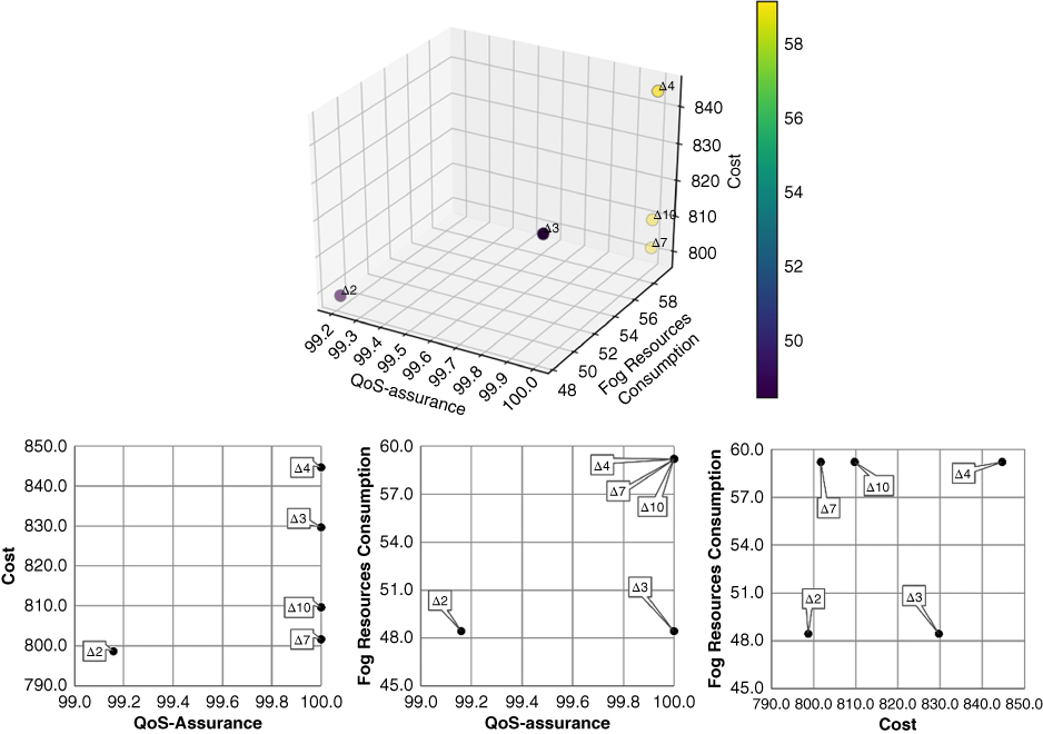
Figure 9.9 Results for Q1(a) and Q1(b).15
Finally, to answer question Q2:
- Q2 — Would there be any deployment that complies with all previous requirements and reduces financial cost and/or consumed fog resources if upgrading from 3G to 4G at Fog 2?
we change the Internet access at Fog 2 from 3G to 4G. This increases the monthly expenses by € 20. Running FogTorchΠ now reveals six new eligible deployments (Δ12 — Δ17) in addition to the previous output. Among those, only Δ16 turns out to meet also the QoS and budget constraints that the system integrators require (Figure 9.10). Interestingly, Δ16 costs € 70 less than the best candidate for Q1(b) (Δ2), whilst sensibly reducing fog resource consumption. Hence, overall, the change from 3G to 4G would lead to an estimated monthly saving of € 50 with Δ16 with respect to Δ2.

Figure 9.10 Results16 for Q2.
The current FogTorchΠ prototype leaves to system integrators the final choice for a particular deployment, permitting them to freely select the “best” trade‐off among QoS‐assurance, resource consumption and cost. Indeed, the analysis of application‐specific requirements (along with data on infrastructure behavior) can lead decision toward different segmentations of an application from the IoT to the cloud, trying to determine the best trade‐off among metrics that describe likely runtime behavior of a deployment and make it possible to evaluate changes in the infrastructure (or in the application) before their actual implementation (what‐if analysis [12]).
9.5 Related Work
9.5.1 Cloud Application Deployment Support
The problem of deciding how to deploy multicomponent applications has been thoroughly studied in the cloud scenario. Projects like SeaClouds [20], Aeolus [21], or Cloud‐4SOA [22], for instance, proposed model‐driven optimized planning solutions to deploy software applications across multiple (IaaS or PaaS) Clouds. [23] proposed using OASIS TOSCA [24] to model IoT applications in Cloud+IoT scenarios.
With respect to the 15 16 cloud paradigm, the fog introduces new problems, mainly due to its pervasive geo‐distribution and heterogeneity, need for connection‐awareness, dynamicity, and support to interactions with the IoT, that were not taken into account by previous work (e.g., [25–27]). Particularly, some efforts in cloud computing considered nonfunctional requirements (mainly e.g., [28, 29]) or uncertainty of execution (as in fog nodes) and security risks among interactive and interdependent components (e.g., [30]). Only recently, [31] has been among the first attempts to consider linking services and networks QoS by proposing a QoS‐ and connection‐aware cloud service composition approach to satisfy end‐to‐end QoS requirements in the cloud.
Many domain‐specific languages (DSLs) have been proposed in the context of cloud computing to describe applications and resources, e.g. TOSCA YAML [24] or JSON‐based CloudML [32]. We aim not to bind to any particular standard for what concerns the specification of software/hardware offerings so that the proposed approach stays general and can potentially exploit suitable extensions (with respect to QoS and IoT) of such DSLs. Also, solutions to automatically provision and configure software components in cloud (or multi‐cloud) scenarios are currently used by the DevOps community to automate application deployment or to lead deployment design choices (e.g., Puppet [33] and Chef [34]).
In the context of IoT deployments, formal modelling approaches have been recently exploited to achieve connectivity and coverage optimization [35, 36], to improved resource exploitation of Wireless Sensors Networks [37], and to estimate reliability and cost of service compositions [38].
Our research aims at complementing those efforts, by describing the interactions among software components and IoT devices at a higher level of abstraction to achieve informed segmentation of applications through the fog – that was not addressed by previous work.
9.5.2 Fog Application Deployment Support
To the best of our knowledge, few approaches have been proposed so far to specifically model fog infrastructures and applications, as well as to determine and compare eligible deployments for an application to an fog infrastructure under different metrics. Service latency and energy consumption were evaluated in [39] for the new fog paradigm applied to the IoT, as compared to traditional cloud scenarios. The model of [39], however, deals only with the behavior of software already deployed over fog infrastructures.
iFogSim [40] is one of the most promising prototypes to simulate resource management and scheduling policies applicable to fog environments with respect to their impact on latency, energy consumption and operational cost. The focus of iFogSim model is mainly on stream‐processing applications and hierarchical tree‐like infrastructures, to be mapped either cloud‐only or edge‐ward so as to compare results. In Section , we will show how iFogSim and FogTorchΠ can be used complementarily to solve deployment challenges.
Building on top of iFogSim, [41] compares different task scheduling policies, considering user mobility, optimal fog resource utilization and response time. [42] presents a distributed approach to cost‐effective application placement, at varying workload conditions, with the objective of optimizing operational cost across the entire infrastructure. Apropos, [43] introduces a hierarchy‐based technique to dynamically manage and migrate applications between cloud and fog nodes. They exploit message passing among local and global node managers to guarantee QoS and cost constraints are met. Similarly, [44] leverages the concept of fog colonies [45] for scheduling tasks to fog infrastructures, whilst minimizing response times. [46] provides a first methodology for probabilistic record‐based resource estimation to mitigate resource underutilization, to enhance the QoS of provisioned IoT services.
All the aforementioned approaches are limited to monolithic or DAG application topologies and do not take into account QoS for the component–component and component–thing interactions, nor historical data about fog infrastructure or deployment behavior. Furthermore, the attempts to explicitly target and support with predictive methodologies the decision‐making process to deploy IoT applications to the fog did not consider matching of application components to the best virtual instance (virtual machine or container), depending on expressed preferences (e.g., cost or energy targets) in this work.
9.5.3 Cost Models
While pricing models for the cloud are quite established (e.g., [18] and references therein), they do not account for costs generated by the exploitation of IoT devices. Cloud pricing models are generally divided into two types, pay‐per‐use and subscription‐based schemes. In [18], based on given user workload requirements, a cloud broker chooses a best VM instance among several cloud providers. The total cost of deployment is calculated considering hardware requirements such as number of CPU cores, VM types, time duration, type of instance (reserved or pre‐emptible), etc.
On the other hand, IoT providers normally process the sensory data coming from the IoT devices and sell the processed information as value added service to the users. [19] shows how they can also act as brokers, acquiring data from different owners and selling bundles. The authors of [19] also considered the fact that different IoT providers can federate their services and create new offers for their end users. Such end users are then empowered to estimate the total cost of using IoT services by comparing pay‐per‐use and subscription‐based offers, depending on their data demand.
More recently, [47] proposed a cost model for IoT+Cloud scenario. Considering parameters such as the type and number of sensors, number of data request and uptime of VM, their cost model can estimate the cost of running an application over a certain period of time. In fog scenarios, however, there is a need to compute IoT costs at a finer level, also accounting for data‐transfer costs (i.e., event‐based).
Other recent studies tackle akin challenges from an infrastructural perspective, either focusing on scalable algorithms for QoS‐aware placement of microdata centers [48], on optimal placement of data and storage nodes that ensures low latencies and maximum throughput, optimizing costs [49], or on the exploitation of genetic algorithms to place intelligent access points at the edge of the network [50].
To the best of our knowledge, our attempt to model costs in the fog scenario is the first that extends cloud pricing schemes to the fog layer and integrates them with costs that are typical of IoT deployments.
9.5.4 Comparing iFogSim and FogTorchΠ
iFogSim [40] is a simulation tool for fog computing scenarios. In this section, we discuss how both iFogSim and FogTorchΠ can be used together to solve the same input scenario (i.e., infrastructure and application). We do so by assessing whether the results of FogTorchΠ are in line with the results obtained with iFogSim. In this section, we review the VR Game case study employed for iFogSim in [40], execute FogTorchΠ over it, and then compare the results obtained by both prototypes.
The VR Game is a latency sensitive smartphone application which allows multiple players to interact with each other through EEG sensors. It is a multi‐component application consisting of three components (viz., client, coordinator and concentrator) (Figure 9.11). To allow players to interact in real time, the application demands a high level of QoS (i.e., minimum latency) in between components. The infrastructure to host the application consists of a single cloud node, an ISP proxy, several gateways, and smartphones connected to EEG sensors (Figure 9.12). The number of gateways is variable and can be set (to 1, 2, 4, 8 or 16), while the number of smartphones connected to each gateway remains constant (viz., 4).

Figure 9.11 VR Game application.

Figure 9.12 VR Game infrastructure.18
For the given input application and infrastructure, iFogSim produces and simulates a single deployment (either cloud‐only or edge‐ward [40]) that satisfies all the specified hardware and software requirements. Simulation captures tuple exchange among components in the application, as in an actual deployment. This enables administrators to compare the average latency of the time‐sensitive control loop 〈EEG‐client‐concentrator‐client‐screen〉 when adopting a cloud‐only or an edge‐ward deployment strategy.
On the other hand, FogTorchΠ produces various eligible deployments 17 for the same input to choose from. Indeed, FogTorchΠ outputs a set of 25 eligible deployments depending on variations in the number of gateways used in the infrastructure.
As shown in Table 9.4, FogTorchΠ output mainly includes edge‐ward deployments for the VR Game application example. This is very much in line with the results obtained with iFogSim in [40], where cloud‐only deployments perform much worse than edge‐ward ones (especially when the number of involved devices – smartphones and gateways – increases). Also, the only output deployments that exploit the cloud as per FogTorchΠ results over this example are Δ2 and Δ5 , featuring a very low QoS‐assurance (< 1%).
Table 9.4 Result of FogTorchΠ for the VR Game.

|
As per [40], iFogSim does not yet feature performance prediction capabilities – such as the one implemented by FogTorchΠ – in its current version. However, such functionalities can be implemented by exploiting the monitoring layer offered by the tool, also including a knowledge base that conserves historical data about the infrastructure behavior.
Summing up, iFogSim and FogTorchΠ can be seen as somewhat complementary tools designed to help end users in choosing how to deploy their fog applications by first predicting properties of a given deployment beforehand and by, afterward, being able to simulate most promising deployment candidates for any arbitrary time duration. The possibility of integrating predicting features of FogTorchΠ with simulation features of iFogSim is indeed in the scope of future research directions. 18
9.6 Future Research Directions
We see several directions for future work on FogTorchΠ. A first direction could be including other dimensions and predicted metrics to evaluate eligible deployments, to refine search algorithms, and to enrich input and output expressiveness. Particularly, it would be interesting to do the following:
- Introduce estimates 19 of energy consumption as a characterizing metric for eligible deployments, possibly evaluating its impact – along with financial costs – on SLAs and business models in fog scenarios,
- Account for security constraints on secure communication, access control to nodes and components, and trust in different providers, and
- Determine mobility of Fog nodes and IoT devices, with a particular focus on how an eligible deployment can opportunistically exploit the (local) available capabilities or guarantee resilience to churn.
Another direction is to tame the exponential complexity of FogTorchΠ algorithms to scale better over large infrastructures, by leading the search with improved heuristics and by approximating metrics estimation.
A further direction could be to apply multiobjective optimization techniques in order to rank eligible deployments as per the estimated metrics and performance indicators, so to automate the selection of a (set of) deployment(s) that best meet end‐user targets and application requirements.
The reuse of the methodologies designed for FogTorchΠ to generate deployments to be simulated in iFogSim is under study. This will permit comparisons of the predicted metrics generated by FogTorchΠ against the simulation results obtained with iFogSim, and it would provide a better validation to our prototype.
Finally, fog computing lacks medium‐ to large‐scale test‐bed deployments (i.e., infrastructure and applications) to test devised approaches. Last, but not least, it would be interesting to further engineer FogTorchΠ and to assess the validity of the prototype over an experimental lifelike testbed that is currently being studied.
9.7 Conclusions
In this chapter, after discussing some of the fundamental issues related to fog application deployment, we presented the FogTorchΠ prototype, as a first attempt to empower fog application deployers with predictive tools that permit to determine and compare eligible context‐, QoS‐ and cost‐aware deployments of composite applications to Fog infrastructures. To do so, FogTorchΠ considers processing (e.g., CPU, RAM, storage, software), QoS (e.g., latency, bandwidth), and financial constraints that are relevant for real‐time fog applications.
To the best of our knowledge, FogTorchΠ is the first prototype capable of estimating the QoS‐assurance of composite fog applications deployments based on probability distributions of bandwidth and latency featured by end‐to‐end communication links. FogTorchΠ also estimates resource consumption in the fog layer, which can be used to minimize the exploitation of certain fog nodes with respect to others, depending on the user needs. Finally, it embeds a novel cost model to estimate multi‐component application deployment costs to IoT+Fog+Cloud infrastructures. The model considers various cost parameters (hardware, software, and IoT), and extends cloud computing cost models to the fog computing paradigm, while taking into account costs associated with the usage of IoT devices and services.
The potential of FogTorchΠ has been illustrated by discussing its application to a smart building fog application, performing what‐if analyses at design time, including changes in QoS featured by communication links and looking for the best trade‐off among QoS‐assurance, resource consumption, and cost.
Needless to say, the future of predictive tools for fog computing application deployment has just started, and much remains to understand how to suitably balance different types of requirements so to make the involved stakeholders aware of the choices to be made throughout application deployment.
References
- 1 CISCO. Fog computing and the Internet of Things: Extend the cloud to where the things are. https://www.cisco.com/c/dam/en_us/solutions/trends/iot/docs/computing‐overview.pdf, 30/03/2018.
- 2 CISCO. Cisco Global Cloud Index: Forecast and Methodology. 2015–2020, 2015.
- 3 A. V. Dastjerdi and R. Buyya. Fog Computing: Helping the Internet of Things Realize Its Potential. Computer , 49(8): 112–116, August 2016.
- 4 I. Stojmenovic, S. Wen, X. Huang, and H. Luan. An overview of fog computing and its security issues. Concurrency and Computation: Practice and Experience , 28(10): 2991–3005, July 2016.
- 5 R. Mahmud, R. Kotagiri, and R. Buyya. Fog computing: A taxonomy, survey and future directions. Internet of Everything: Algorithms, Methodologies, Technologies and Perspectives, Beniamino Di Martino, Kuan‐Ching Li, Laurence T. Yang, Antonio Esposito (eds.), Springer, Singapore, 2018.
- 6 F. Bonomi, R. Milito, P. Natarajan, and J. Zhu. Fog computing: A platform for internet of things and analytics. Big Data and Internet of Things: A Roadmap for Smart Environments, N. Bessis, C. Dobre (eds.), Springer, Cham, 2014.
- 7 W. Shi and S. Dustdar. The promise of edge computing. Computer , 49(5): 78–81, May 2016.
- 8 A. Brogi and S. Forti. QoS‐aware Deployment of IoT Applications Through the Fog. IEEE Internet of Things Journal , 4(5): 1185–1192, October 2017.
- 9 P. O. Östberg, J. Byrne, P. Casari, P. Eardley, A. F. Anta, J. Forsman, J. Kennedy, T.L. Duc, M.N. Mariño, R. Loomba, M.Á.L. Peña, J.L. Veiga, T. Lynn, V. Mancuso, S. Svorobej, A. Torneus, S. Wesner, P. Willis and J. Domaschka. Reliable capacity provisioning for distributed cloud/edge/fog computing applications. In Proceedings of the 26th European Conference on Networks and Communications, Oulu, Finland, June 12–15, 2017.
- 10 OpenFog Consortium. OpenFog Reference Architecture (2016), http://openfogconsortium.org/ra, 30/03/2018.
- 11 M. Chiang and T. Zhang. Fog and IoT: An overview of research opportunities. IEEE Internet of Things Journal, 3(6): 854–864, December 2016.
- 12 S. Rizzi, What‐if analysis. Encyclopedia of Database Systems, Springer, US, 2009.
- 13 A. Brogi, S. Forti, and A. Ibrahim. How to best deploy your fog applications, probably. In Proceedings of the 1st IEEE International Conference on Fog and Edge Computing, Madrid, Spain, May 14, 2017.
- 14 A. Brogi, S. Forti, and A. Ibrahim. Deploying fog applications: How much does it cost, by the way? In Proceedings of the 8th International Conference on Cloud Computing and Services Science, Funchal (Madeira), Portugal, March 19–21, 2018.
- 15 C. Perera. Sensing as a Service for Internet of Things: A Roadmap. Leanpub, Canada, 2017.
- 16 S. Newman. Building Microservices: Designing Fine‐Grained Systems. O'Reilly Media, USA, 2015.
- 17 W. L. Dunn and J. K. Shultis. Exploring Monte Carlo Methods. Elsevier, Netherlands, 2011.
- 18 J. L. Dìaz, J. Entrialgo, M. Garcìa, J. Garcìa, and D. F. Garcìa. Optimal allocation of virtual machines in multi‐cloud environments with reserved and on‐demand pricing, Future Generation Computer Systems, 71: 129–144, June 2017.
- 19 D. Niyato, D. T. Hoang, N. C. Luong, P. Wang, D. I. Kim and Z. Han. Smart data pricing models for the internet of things: a bundling strategy approach, IEEE Network 30(2): 18–25, March–April 2016.
- 20 A. Brogi, A. Ibrahim, J. Soldani, J. Carrasco, J. Cubo, E. Pimentel and F.D'Andria. SeaClouds: a European project on seamless management of multi‐cloud applications. Software Engineering Notes of the ACM Special Interest Group on Software Engineering , 39(1): 1–4, January 2014.
- 21 R.Di Cosmo, A. Eiche, J. Mauro, G. Zavattaro, S. Zacchiroli, and J. Zwolakowski. Automatic Deployment of Software Components in the cloud with the Aeolus Blender. In Proceedings of the 13th International Conference on Service‐Oriented Computing, Goa, India, November 16–19, 2015.
- 22 A. Corradi, L. Foschini, A. Pernafini, F. Bosi, V. Laudizio, and M.Seralessandri. Cloud PaaS brokering in action: The Cloud4SOA management infrastructure. In Proceedings of the 82nd IEEE Vehicular Technology Conference, Boston, MA, September 6–9, 2015.
- 23 F. Li, M. Voegler, M. Claesens, and S. Dustdar. Towards automated IoT application deployment by a cloud‐based approach. In Proceedings of the 6th IEEE International Conference on Service‐Oriented Computing and Applications, Kauai, Hawaii, December 16–18, 2013.
- 24 A. Brogi, J. Soldani and P. Wang. TOSCA in a Nutshell: Promises and Perspectives. In Proceedings of the 3rd European Conference on Service‐Oriented and Cloud Computing, Manchester, UK, September 2–4, 2014.
- 25 P. Varshney and Y. Simmhan. Demystifying fog computing: characterizing architectures, applications and abstractions. In Proceedings of the 1st IEEE International Conference on Fog and Edge Computing, Madrid, Spain, May 14, 2017.
- 26 Z. Wen, R. Yang, P. Garraghan, T. Lin, J. Xu, and M. Rovatsos. Fog orchestration for Internet of Things services. iEEE Internet Computing , 21(2): 16–24, March–April 2017.
- 27 J.‐P. Arcangeli, R. Boujbel, and S. Leriche. Automatic deployment of distributed software systems: Definitions and state of the art. Journal of Systems and Software , 103: 198–218, May 2015.
- 28 R. Nathuji, A. Kansal, and A. Ghaffarkhah. Q‐Clouds: Managing Performance Interference Effects for QoS‐Aware Clouds. In Proceedings of the 5th EuroSys Conference, Paris, France, April 13–16, 2010.
- 29 T. Cucinotta and G.F. Anastasi. A heuristic for optimum allocation of real‐time service workflows. In Proceedings of the 4th IEEE International Conference on Service‐Oriented Computing and Applications, Irvine, CA, USA, December 12–14, 2011.
- 30 Z. Wen, J. Cala, P. Watson, and A. Romanovsky. Cost effective, reliable and secure workflow deployment over federated clouds. IEEE Transactions on Services Computing , 10(6): 929–941, November–December 2017.
- 31 S. Wang, A. Zhou, F. Yang, and R. N. Chang. Towards network‐aware service composition in the cloud. IEEE Transactions on Cloud Computing, August 2016.
- 32 A. Bergmayr, A. Rossini, N. Ferry, G. Horn, L. Orue‐Echevarria, A. Solberg, and M. Wimmer. The Evolution of CloudML and its Manifestations. In Proceedings of the 3rd International Workshop on Model‐Driven Engineering on and for the Cloud, Ottawa, Canada, September 29, 2015.
- 33 Puppetlabs, Puppet, https://puppet.com. Accessed March 30, 2018.
- 34 Opscode, Chef, https://www.chef.io. Accessed March 30, 2018.
- 35 J. Yu, Y. Chen, L. Ma, B. Huang, and X. Cheng. On connected Target k‐Coverage in heterogeneous wireless sensor networks. Sensors, 16(1): 104, January 2016.
- 36 A.B. Altamimi and R.A. Ramadan. Towards Internet of Things modeling: a gateway approach. Complex Adaptive Systems Modeling , 4(25): 1–11, November 2016.
- 37 H. Deng, J. Yu, D. Yu, G. Li, and B. Huang. Heuristic algorithms for one‐slot link scheduling in wireless sensor networks under SINR. International Journal of Distributed Sensor Networks , 11(3): 1–9, March 2015.
- 38 L. Li, Z. Jin, G. Li, L. Zheng, and Q. Wei. Modeling and analyzing the reliability and cost of service composition in the IoT: A probabilistic approach. In Proceedings of 19th International Conference on Web Services, Honolulu, Hawaii, June 24–29, 2012.
- 39 S. Sarkar and S. Misra. Theoretical modelling of fog computing: a green computing paradigm to support IoT applications. IET Networks , 5(2): 23–29, March 2016.
- 40 H. Gupta, A.V. Dastjerdi, S.K. Ghosh, and R. Buyya. iFogSim: A Toolkit for Modeling and Simulation of Resource Management Techniques in Internet of Things, Edge and Fog Computing Environments. Software Practice Experience , 47(9): 1275–1296, June 2017.
- 41 L.F. Bittencourt, J. Diaz‐Montes, R. Buyya, O.F. Rana, and M. Parashar, Mobility‐aware application scheduling in fog computing. IEEE Cloud Computing, 4(2): 26–35, April 2017.
- 42 W. Tarneberg, A.P. Vittorio, A. Mehta, J. Tordsson, and M. Kihl, Distributed approach to the holistic resource management of a mobile cloud network. In Proceedings of the 1st IEEE International Conference on Fog and Edge Computing, Madrid, Spain, May 14, 2017.
- 43 S. Shekhar, A. Chhokra, A. Bhattacharjee, G. Aupy and A. Gokhale, INDICES: Exploiting edge resources for performance‐aware cloud‐hosted services. In Proceedings of the 1st IEEE International Conference on Fog and Edge Computing, Madrid, Spain, May 14, 2017.
- 44 O. Skarlat, M. Nardelli, S. Schulte and S. Dustdar. Towards QoS‐aware fog service placement. In Proceedings of the 1st IEEE International Conference on Fog and Edge Computing, Madrid, Spain, May 14, 2017.
- 45 O. Skarlat, S. Schulte, M. Borkowski, and P. Leitner. Resource Provisioning for IoT services in the fog. In Proceedings of the 9th IEEE International Conference on Service‐Oriented Computing and Applications, Macau, China, November 4–6, 2015.
- 46 M. Aazam, M. St‐Hilaire, C. H. Lung, and I. Lambadaris. MeFoRE: QoE‐based resource estimation at Fog to enhance QoS in IoT. In Proceedings of the 23rd International Conference on Telecommunications, Thessaloniki, Greece, May 16–18, 2016.
- 47 A. Markus, A. Kertesz and G. Kecskemeti. Cost‐Aware IoT Extension of DISSECT‐CF, Future Internet, 9(3): 47, August 2017.
- 48 M. Selimi, L. Cerdà‐Alabern, M. Sànchez‐Artigas, F. Freitag and L. Veiga. Practical Service Placement Approach for Microservices Architecture. In Proceedings of the 17th IEEE/ACM International Symposium on Cluster, Cloud and Grid Computing, Madrid, Spain, May 14–17, 2017.
- 49 I. Naas, P. Raipin, J. Boukhobza, and L. Lemarchand. iFogStor: an IoT data placement strategy for fog infrastructure. In Proceedings of the 1st IEEE International Conference on Fog and Edge Computing, Madrid, Spain, May 14, 2017.
- 50 A. Majd, G. Sahebi, M. Daneshtalab, J. Plosila, and H. Tenhunen. Hierarchal placement of smart mobile access points in wireless sensor networks using fog computing. In Proceedings of the 25th Euromicro International Conference on Parallel, Distributed and Network‐based Processing, St. Petersburg, Russia, March 6–8, 2017.
- 51 K. Fatema, V.C. Emeakaroha, P.D. Healy, J.P. Morrison and T. Lynn. A survey of cloud monitoring tools: Taxonomy, capabilities and objectives. Journal of Parallel and Distributed Computing, 74(10): 2918–2933, October 2014.
- 52 Y. Breitbart, C.‐Y. Chan, M. Garofalakis, R. Rastogi, and A. Silberschatz. Efficiently monitoring bandwidth and latency in IP networks. In Proceedings of the 20th Annual Joint Conference of the IEEE Computer and Communications Societies, Alaska, USA, April 22–26, 2001.