
6 Computer vision: Object recognition
- Vectorizing images into quantitative features for ML
- Using pixel values as features
- Extracting edge information from images
- Fine-tuning deep learning models to learn optimal image representations
Continuing our journey through dealing with unstructured data leads us to our image case study. Just as it was an issue with our NLP case study, the big question of this chapter is, how do we represent images in a machine-readable format? Throughout this chapter, we will take a look at ways to construct, extract, and learn feature representations of images for the purpose of solving an object recognition problem.
Object recognition simply means we are going to work with labeled images, where each image contains a single object, and the purpose of the model is to classify the image as a category that specifies what object is in the image. Object recognition is considered a relatively simple computer vision problem, as we don’t have to worry about finding the object or objects within an image using bounding boxes, nor do we have to do anything beyond pure classification into (usually) mutually exclusive categories. Let’s jump right into taking a look at the dataset for this case study—the CIFAR-10 dataset.
Warning This chapter also has some long-running code samples throughout the chapter. Working with images can be cumbersome due to file sizes and the memory required to keep them in memory. Be advised that some code samples may run for over an hour on the minimum requirements for this book.
6.1 The CIFAR-10 dataset
The CIFAR-10 dataset is used widely for training object recognition architectures. According to the website dedicated to hosting the data, it consists of 60,000 32 × 32 color images, which are split up into 10 classes, each with 6,000 images. There are 50,000 training images and 10,000 test images. There are instructions on the site for how to parse the data, so let’s use that to load up the data ourselves in the following listing.
Listing 6.1 Ingesting the CIFAR-10 data
def unpickle(file):                                                            ❶
    with open(file, 'rb') as fo:
        d = pickle.load(fo, encoding='bytes')
    return d

def load_cifar(filenames):
    training_images = []
    training_labels = []

    for file_name in filenames:
        unpickled_images = unpickle(file_name)
        images, labels = unpickled_images[b'data'], unpickled_images[b'labels']❷
        images = np.reshape(images,(-1, 3, 32, 32))                            ❸
        images = np.transpose(images, (0, 2, 3, 1))                            ❸
        training_images.append(images)
        training_labels += labels

    return np.vstack(training_images), training_labels

print("Loading the training set")
training_files = [f'../data/cifar-10/data_batch_{i}'
                  for i in range(1, 6)]  # D
training_images, int_training_labels = load_cifar(
    training_files)

print("Loading the testing set")
training_files = ['../data/cifar-10/test_batch']                               ❹
testing_images, int_testing_labels = load_cifar(
    training_files)

print("Loading the labels")
label_names = unpickle(
    '../data/cifar-10/batches.meta')[b'label_names']                           ❺
training_labels = [str(label_names[_]) for _ in int_training_labels]
testing_labels = [str(label_names[_]) for _ in int_testing_labels]
❶ Function to load the files from the main CIFAR site
❷ Grab the images and labels from the files.
❸ Reshape and transpose, so our shape is (number_of_images, height, width, channels [RGB]).
❹ Load up the training and testing images.
Now, we can try taking a look at our images:
import matplotlib.pyplot as plt
print(training_labels[0])
plt.imshow(training_images[0])
Each image is a 32 x 32 image with each pixel containing values for RGB. These three values are also known as channels. Note that if an image only has one channel, that image will be black and white. Each image, therefore, has the shape (32, 32, 3): 32 pixels high, 32 pixels wide, with each pixel containing 3 values for RGB between 0 and 255. So each image is being represented by 3,072 values.
6.1.1 The problem statement and defining success
We are performing yet another classification here, but this time we are classifying 10 classes (figure 6.1). The goal of our model can be summarized by the following question: given a raw image, can we find ways to represent the image and classify the object in the image accurately?

Figure 6.1 The first training image in the CIFAR-10 dataset is a frog. The CIFAR-10 dataset has 10 classes: airplane, automobile, bird, cat, deer, dog, frog, horse, ship, and truck.
The goal of this case study is to find different ways to convert our images into machine-readable features and use those features to train a model. Just like in the last case, the NLP study, we will stick to using a simple logistic regression classifier to ensure that boosts in our ML pipeline performance are due mostly to our feature engineering efforts.
6.2 Feature construction: Pixels as features
Our first attempt to represent our images in a machine-readable format will be to use the pixel values directly as our features. To do this, we will take the mean pixel value (MPV) of the channels and then realign the values to be one-dimensional, rather than two-dimensional. A visualization of this method can be found in the following figure.
Using the mean pixel value happens in two steps:
This simple process will give us a 1,024-length (32 x 32) vector of features we can feed into our model (figure 6.2).

Figure 6.2 The MPV approach converts images into arrays by averaging the red, green, and blue pixel matrices into a single matrix of averaged color values and then realigning the average-color matrix to be a single dimension per image.
We can now test these features against our ML pipeline. Just as we did in the last case study, we will be testing each of our image vectorization techniques against a simple grid search of a logistic regression. Our goal, once again, is to provide a semiconsistent ML model pipeline, where the changing element is our feature engineering efforts. This will give us a sense of how our efforts are paying off.
Let’s run some code to calculate our mean pixel value features. The following code snippet will do just that!
Listing 6.2 Calculating mean pixel values
avg_training_images = training_images.mean(   ❶
    axis=3).reshape(50000,-1)                 ❶
avg_testing_images = testing_images.mean(     ❶
    axis=3).reshape(10000,-1)                 ❶

print(avg_training_images.shape)
❶ Average the RGB values together, and reshape them to make a 1D vector for each image.
We now have a training matrix of size (50,000, 1,024) and a testing matrix of size (10,000, 1,024). Let’s run our grid search code (listing 6.3) to train our logistic regression on our mean pixel values. Remember that the goal of this case study is to find the best representation of an image, and our methodology is to grid search a few parameter options on a logistic regression and use the resulting accuracy on the test set as a metric for how well our feature engineering efforts have done.
NOTE Fitting models in this chapter may take some time to run. For my 2021 MacBook Pro, some of these code segments took over an hour to complete the grid search.
Listing 6.3 Baseline model: using average pixel values as features
from sklearn.pipeline import Pipeline
from sklearn.linear_model import LogisticRegression               ❶

clf = LogisticRegression(max_iter=100, solver='saga')             ❷

ml_pipeline = Pipeline([                                          ❸
    ('classifier', clf)
])

params = {  # C                                                   ❸
    'classifier__C': [1e-1, 1e0, 1e1]
}

print("Average Pixel Value + LogReg
==========================")
advanced_grid_search(                                             ❹
    avg_training_images, training_labels, avg_testing_images, testing_labels,
    ml_pipeline, params
)
❷ Instantiate our simple LogisticRegression model.
❸ Set up our simple grid-search pipeline to try three different values for the logistic regression model.
❹ Run our grid search to get an accuracy value for our pipeline.
The result is that it took the machine running the code (a 2021 MacBook Pro with 16 GB RAM and no GPU) about 20 minutes in total to run a grid search of only three parameters, and the best accuracy it could come up with is 26% (figure 6.3). This is not so great, but this gives us a good baseline model to beat. At the end of this chapter, we will recap all of the image vectorization methods we saw and how they compared to each other.

Figure 6.3 Just like in our last case study, we will focus on the overall accuracy of our test set as our metric of choice. Our MPV approach is not that predictively powerful but will provide a baseline accuracy to beat of 26%. We could look at the individual precision and recall scores of each class if we believed single classes were more important than others, but we will assume the overall accuracy of the model is what we value the most.
Taking raw pixel values as direct features is unstable and will likely never be the best representation of images for modern computer vision problems. Let’s move on now to a more industry-standard approach to extracting features from images: histograms of oriented gradients.
6.3 Feature extraction: Histogram of oriented gradients
In our last section, we were using raw pixel values as features, and that did not lead to great results. In this section, we will see how histograms of oriented gradients (HOGs) will fare. HOG is a feature extraction technique that is used most commonly for object recognition tasks. HOG focuses on the shape of the object in the image by attempting to quantify the gradient (or magnitude) as well as the orientation (or direction) of the edges of the object.
HOG will calculate gradients and orientations in broken-down, localized regions of the image and calculate a histogram of gradients and orientations to determine the final feature values. This is why the process is known as HOGs.
The process works in five steps:
-
(Optional) Apply a global image normalization. This can come in the form of a gamma compression by taking the square root or log of each color channel. This step provides protection from illumination effects (having different lighting in the images could add noise to the model, for example) and can also help reduce the effects of local shadowing.
-
Compute image gradients in the x and y directions, and use the gradient to compute the magnitude—how quickly the image is changing—and orientation—in which direction the image is changing most rapidly. Gradients capture texture information, contour/edge information, and more. We use the locally dominant color channel (whichever color is the most intense in the region) to help reduce color variance effects. We can set the size of the localized regions using a parameter called pixels_per_cell.
-
Calculate one-dimensional orientation histograms across the cells of the image. The number of bins is a parameter we can set called orientations. The minor difference between a normal histogram and HOG is that instead of counting one instance in a bin like we normally would, we use the magnitude to vote in the histogram. This gives focal points in the image more power in our final feature set.
-
(Optional) Calculate normalization across blocks. This is done by applying some function to the histogram in each block to protect even further against illuminance variation, shadowing, and edge contrasts. The size of a block can be changed by altering the cells_per_block parameters. The normalized block descriptors are referred to as our HOG descriptors.
-
Collect the HOG descriptors, and concatenate them into a final one-dimensional feature vector to represent the entire image.
We can perform these five steps quickly using the scikit-image package. Let’s see an example of HOGs on our training images. To do this, we will set a few parameters:
-
pixels_per_cell=(4, 4) to set our cell size to be 4 pixels by 4 pixels
-
cells_per_block=(2, 2) to set our block size to be 2 cells by 2 cells or 8 pixels by 8 pixels
-
transform_sqrt=True to apply a global preprocessing step to normalize the image values
A quick note about the values for orientations, pixels per cell, and cells per block: we choose these values fairly arbitrarily as a baseline. We could have done more work to find optimal values for each of these parameters, but we will quickly move on to more state-of-the-art techniques. We wanted to highlight HOG features as a great baseline for image vectors, and in some simpler computer vision cases they can be optimal for speed and efficiency. We can think of HOG features similarly to the bag-of-words (BOW) vectorizers in the last chapter. HOG and BOW are both older ways to vectorize images and text, respectively, and we use them as starting points.
More information about these parameters can be found on the main page for the HOG featurizer on scikit-image’s documentation: https://scikit-image.org/docs/0.15.x/api/skimage.feature.html. For now, let’s move on to the following listing, where we can visualize HOG features for our CIFAR data.
Listing 6.4 Visualizing HOGs in CIFAR-10
from skimage.feature import hog                              ❶
from skimage import data, exposure                           ❶
from skimage.transform import resize                         ❶

for image in training_images[:3]:

    hog_features, hog_image = hog(                           ❷
        image,
        orientations=8, pixels_per_cell=(4, 4), cells_per_block=(2, 2),
        channel_axis=-1, transform_sqrt=True,
        block_norm='L2-Hys', visualize=True)

    fig, (ax1, ax2) = plt.subplots(
        1, 2, figsize=(4, 4), sharex=True, sharey=True)
                                                             ❸
    ax1.axis('off')                                          ❸
    ax1.imshow(image, cmap=plt.cm.gray)                      ❸
    ax1.set_title('Input image')                             ❸

    ax2.axis('off')                                          ❸
    ax2.imshow(hog_image, cmap=plt.cm.gray)                  ❸
    ax2.set_title('Histogram of Oriented Gradients')         ❸

print(hog_features.shape)                                    ❹
plt.show()
❶ Import functions from scikit-image.
❷ Calculate HOG for three of our training images.
❸ Plot the HOG next to the original images.
❹ The size of the feature vector
Figure 6.4 shows a list of a few CIFAR images, with the original image on the left and a visualized HOG image on the right. We can see the outlines and movement in the HOG images without much of the background noise (pun intended).
NOTE When calculating HOGs, it is generally best practice to resize images to be of a scale 1:2 (e.g., 32 x 64), but because our images are so small already, we chose not to do this to not lose any valuable information. The HOG calculation will still work just fine!

Figure 6.4 A sample of CIFAR-10 images with their accompanying HOG visualizations. Each cell shows us the most dramatic directions of movement to highlight edges in the image. The HOG visualizations are a lower-fidelity representation of their original raw images that will provide the input to our ML model.
Let’s now create a helper function (listing 6.5) to batch convert our training and testing images into HOG features, using the parameters we set in listing 6.4. If we wanted to, we could set up a custom scikit-learn transformer to accomplish the same effect; however, because this conversion to HOG features is independent of anything else in our ML pipeline, it’s quicker to simply convert the entire training and testing matrices into HOG matrices before running any ML. The following code snippet will do that for us.
Listing 6.5 Calculating HOGs for CIFAR-10
from tqdm import tqdm           ❶
def calculate_hogs(images):     ❷
    hog_descriptors = []
    for image in tqdm(images):
        hog_descriptors.append(hog(
            image, orientations=8, pixels_per_cell=(4, 4),
            cells_per_block=(2, 2), transform_sqrt=True,
            channel_axis=-1, block_norm='L2-Hys',
            visualize=False
        ))

    return np.squeeze(hog_descriptors)

hog_training = calculate_hogs(training_images)
hog_testing = calculate_hogs(testing_images)
❶ tqdm will give us a progress bar, so we can see how long it takes to calculate our HOGs.
❷ Function to calculate HOGs for a set of images
Now that we have our HOG features, let’s test how well those features represent our images by training our ML pipeline on them in the following listing.
Listing 6.6 Using HOGs as features
print("HOG + LogReg
=====================")
advanced_grid_search(
    hog_training, training_labels, hog_testing, testing_labels,
    ml_pipeline, params
)
Taking a look at the following figure, we see an immediate improvement in performance, using HOG features over raw pixel values, from 26% to 56% overall accuracy. Of course, we will not be satisfied with 56% accuracy (figure 6.5), but it’s definitely an improvement! One minor drawback is that the time it takes to run our grid search code has gone up, implying that our model will likely run a bit slower. This is partly due to the fact that we are working with a larger number of overall features. Utilizing the raw pixel values yielded 1,024 features, while HOG produced over 1,500 features.

Figure 6.5 Results from using HOG features show an increase in performance to 56% accuracy from our previous 26%. While 56% is not an incredible accuracy score, it’s worth noting that we are asking our model to pick between 10 categories. We can also see an overall slowdown in the model due to the increase in number of features being learned from.
If only there was a way to capture the representation from HOG features, while reducing the feature complexity. Oh wait, we saw an example of this in the last chapter! Let’s see if we can use dimension reduction techniques to reduce the complexity of our pipeline.
6.3.1 Optimizing dimension reduction with PCA
We’ve seen dimension reduction in action in the last chapter when we were working with the truncated SVD module in scikit-learn. We can bring the same idea here in an effort to reduce the number of features our logistic regression model needs to learn from, while retaining the representation we have from HOG.
Let’s take a different approach from the last chapter. Instead of grid searching to find an optimal value, let’s run a principal component analysis (PCA) on the HOG representation before running any ML code. Then, let’s find the optimal number of components to use and then reduce the dimensions before running our logistic regression model on it. The following listing will run a PCA on the HOG features and output the amount of cumulative explained variance for every additional principal component used.
Listing 6.7 Dimension reduction with PCA
from sklearn.decomposition import PCA                  ❶

num_hog_features = hog_training.shape[1]               ❷

p = PCA(n_components=num_hog_features)                 ❸
p.fit(hog_training)                                    ❸

plt.plot(p.explained_variance_ratio_.cumsum())         ❹
plt.title('Explained Variance vs # of PCA Components')
plt.xlabel('Number of Components')
plt.ylabel('% of Explained Variance')
❶ Import our principal component analysis module.
❷ Number of features from the original HOG transformation
❸ Fit the PCA module to the HOG matrix.
❹ Visualize the cumulative explained variance.
The resulting graph (figure 6.6) will show us how much of the variance in the original data is being captured with every additional dimension. Our job is now to pick a number of components we believe will satisfactorily represent the original HOG features. From the graph, it seems that 600 components is likely a reasonable choice. The percent of explained variance is near 100%, and 600 is over 60% fewer features than our original HOG feature set. It feels like a great idea to choose 600 as our optimal component size, then!
Exercise 6.1 Find the cumulative percent of explained variance, using 10, 100, 200, and 400 principal components.
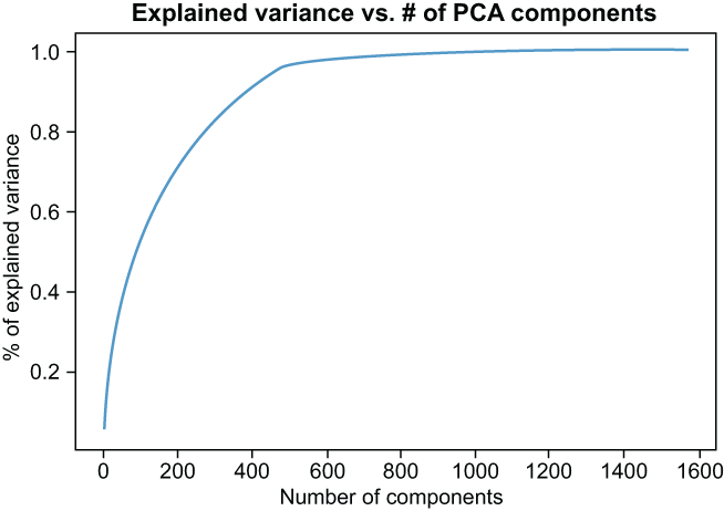
Figure 6.6 The PCA graph reveals that around 600 components should be enough to capture the information from the HOG features, while cutting down on features by 60%.
Now that we’ve chosen 600 as the number of features we wish to reduce down to, let’s reduce our HOG features to 600 dimensions and rerun our grid search function in the following listing.
Listing 6.8 Using reduced HOG dimensions as features
p = PCA(n_components=600)                           ❶

hog_training_pca = p.fit_transform(hog_training)    ❷
hog_testing_pca = p.transform(hog_testing)          ❷

print("HOG + PCA + LogReg
=====================")
advanced_grid_search(                               ❸
    hog_training_pca, training_labels, hog_testing_pca, testing_labels,
    ml_pipeline, params
)
❶ Choose to extract 600 new features.
❷ Transform the original HOG features to the reduced space.
❸ Get accuracy for reduced HOG features.
The results are promising in figure 6.7! We did not lose any overall predictive power by looking at the model’s accuracy on the test set, and the code ran over 75% faster (the last run took over 1,480 seconds to run, while this run took just under 390 seconds), implying our model is learning and predicting much more quickly. This is an excellent example of dimension reduction techniques like PCA and SVD working well!

Figure 6.7 Applying PCA to our HOG features yields the same accuracy, but the pipeline complexity has dramatically been reduced, as evidenced by the amount of time it takes to run our grid search decreasing by 75%. It is safe to say that this model is faster and just as accurate.
So far every technique we have tried has led to better results in either bolstering predictive power or reducing model and feature complexity. In our last chapter, we saw the best results coming from state-of-the-art feature learning by way of transfer learning. Let’s now turn our sights to our final section of the study, where we introduce another transfer learning-based model to see if the same will hold true here.
Both the mean pixel feature approach and the HOG extractor are excellent quick transformations of images with extensive histories of working relatively well in certain situations. Let’s move on into more state-of-the-art feature learning techniques with our newest transfer learning model.
6.4 Feature learning with VGG-11
As we mentioned previously, HOG features and BOW features for NLP datasets are still used by many folks in the field but are rapidly being replaced by more state-of-the-art, deep learning, feature learning and extraction techniques. For our NLP case study, we relied on the mighty BERT, and for images, we will turn our attention to the transfer learning model called the VGG-11 model from the VGG family of models.
VGG stands for a group at Oxford called the Visual Geometry Group (https://www.robots.ox.ac.uk/~vgg), which originally architected this family in 2014 and used it to participate in an object recognition task that focused around the ImageNet dataset, another object recognition dataset like CIFAR-10. VGG models are Convolutional Neural Networks (ConvNets) and rely heavily on convolutional and pooling layers to represent images in the network. Convolutional layers will apply some filter/kernel, which is a function applied to localized regions of the 3D input, and output another set of 3D results. Figure 6.8 shows a high-level view of a ConvNet compared to a traditional feedforward neural network. Pooling layers periodically reduce the size of the representation to promote faster learning and prevent overfitting. These filters are considered learnable parameters, so the goal of the ConvNet is to learn what filters (functions) are best for extracting useful information about localized regions of the image for a given task. If we think back to the HOG section, we were applying a specific gradient or orientation filter to extract edge information from the image. ConvNets are trying to learn what types of filters are best for a given task without being told explicitly what filters to apply.

Figure 6.8 The left image shows a traditional neural network. The right image is of a convolutional network. The ConvNet will arrange neurons into three dimensions. Each subsequent layer of a ConvNet will map the 3D input to another 3D output of activations.
The VGG family of architectures have two main sections in their networks: a feature learning section and a classifier. The feature learning section of the network uses the convolutional and pooling layers to learn useful representations of images. The classifier section maps these representations to a set of labels to perform the classification. The pretrained version on ImageNet will map to one of 1,000 labels in the dataset.
VGG-11 is among the smaller of the VGG models, and its name comes from the fact that there are 11 weight layers in the model: 8 convolutional layers in the feature learning section and 3 feedforward layers in the classifier section. The 8 convolutional layers are specifically to learn functional filters that best represent the image, while the 3 feedforward layers convert that representation into a label classification task. Figure 6.9 shows a visualization of all layers of the VGG-11 model.

Figure 6.9 The VGG family of architectures with two main sections. The feature learning section of the network is built using convolutional and pooling layers with ReLU activations.
6.4.1 Using a pretrained VGG-11 as a feature extractor
Wait, what did he say? Feature extractor? I thought this was the feature learning section. It is, but we will be taking the feature learning section of the VGG-11 model that was trained on the ImageNet database and using it to map our images to the pretrained 512-length feature vector. Our hope is that the feature learning that happened during training will transfer over to being a good image vectorization function for our purposes.
NOTE We are not using the VGG-11 to the exact specifications that its authors intended here. The authors use images that are 224 x 224 pixels to train the original model, and ours are only 32 x 32, for example. It is not imperative that we always strictly follow the author’s intentions, but it is always good to know which assumptions we are explicitly breaking, so if our model tends to underperform, we have an idea of what may be going wrong.
In listing 6.9, let’s load up the VGG-11 model the same way we loaded BERT in the last chapter. Let’s, then, standardize our images according to a learned mean and standard deviation taken directly from the VGG paper. Recall that, by standardization, we simply mean calculating the z-score for each pixel value, where the mean and standard deviation have already been learned offline.
Listing 6.9 Loading a pretrained VGG-11 model and standardize images
import torchvision.models as models
import torch.nn as nn

vgg_model = models.vgg11(pretrained='imagenet')                             ❶

normalized_training_images = ((training_images/255) - [0.485, 0.456, 0.406])❷
➥ / [0.229, 0.224, 0.225]                                                  ❷
normalized_testing_images = ((testing_images/255) - [0.485, 0.456, 0.406]) /❷
➥ [0.229, 0.224, 0.225]                                                    ❷
❶ Instantiate a VGG-11 model pretrained on the imagenet corpus.
❷ Normalize the raw images, using values from the original paper.
We can take a look at the model itself and see for ourselves the 11 weight layers in the model in figure 6.10.

Figure 6.10 VGG-11 has 11 weight layers: 8 convolutional layers in the features section and 3 feedforward layers in the classifier section.
Now that we have our data standardized and our model loaded up, we need to do a bit more housekeeping by transforming our images into DataLoaders, which are classes in PyTorch designed to load data in batches. The model is expecting our images to also be of a different shape with the channels dimension first, rather than at the end, as we’ve had it so far.
I promise that the results will be worth it! Let’s load our data into DataLoaders in listing 6.10. The steps in general for both training and testing data are
-
Transpose the image matrices, so we have the number of images first, the channels second, and then the height and width.
-
Load the tensor/matrix into a DataSet along with the labels.
-
Instantiate a DataLoader with our newly created DataSet, setting the shuffle parameter to true with a batch size of 2,048.
Listing 6.10 Loading the data into PyTorch DataLoaders
import torch
from torch.utils.data import TensorDataset, DataLoader

training_images_tensor =
torch.Tensor(normalized_training_images.transpose(0, 3, 1, 2))   ❶
training_labels_tensor =                                         ❶
torch.Tensor(int_training_labels).type(torch.LongTensor)         ❶

training_dataset = TensorDataset(training_images_tensor,         ❶
training_labels_tensor)                                          ❶
training_dataloader = DataLoader(training_dataset,               ❶
shuffle=True, batch_size=2048)                                   ❶


testing_images_tensor = torch.Tensor(normalized_testing_images   ❷
.transpose(0, 3, 1, 2))                                          ❷
testing_labels_tensor =                                          ❷
torch.Tensor(int_testing_labels).type(torch.LongTensor)          ❷

testing_dataset = TensorDataset(testing_images_tensor,           ❷
testing_labels_tensor)                                           ❷
testing_dataloader = DataLoader(testing_dataset,                 ❷
shuffle=True, batch_size=2048)                                   ❷
❶ Transform the normalized training image data into a PyTorch DataLoader.
❷ Transform the normalized testing image data into a PyTorch DataLoader.
We’re almost ready to extract features! Let’s create a helper function that will take batches of data from our DataLoaders and run them through the VGG-11 feature section of the model. Our next code listing will do just that! It will
-
Take in a feature_extractor as an input, which, itself, can take in iterables of images and output a matrix of features.
-
For each batch, it will pass the image into the feature_extractor and then detach and convert the output to a NumPy array with only two dimensions (batch_size and feature_vector_length).
-
Run steps 2 and 3 for both the training DataLoader and the testing DataLoader.
We will aggregate them all into a final matrix in listing 6.11. Keep in mind that even though this model is among the smaller in the family, it is still over half a gigabyte large and can be a bit slow!
Listing 6.11 Helper function to aggregate training and testing matrices
from tqdm import tqdm

def get_vgg_features(feature_extractor):
    print("Extracting features for training set")
    extracted_training_images = []
    shuffled_training_labels = []
    for batch_idx, (data_, target_) in tqdm(enumerate(training_dataloader)):
        extracted_training_images.append(
            feature_extractor(
                data_).detach().numpy().squeeze((2, 3)))
        shuffled_training_labels += target_

    print("Extracting features for testing set")
    extracted_testing_images = []
    shuffled_testing_labels = []
    for batch_idx, (data_, target_) in tqdm(enumerate(testing_dataloader)):
        extracted_testing_images.append(
            feature_extractor(
                data_).detach().numpy().squeeze((2, 3)))
        shuffled_testing_labels += target_

    return np.vstack(extracted_training_images),
           shuffled_training_labels,
           np.vstack(extracted_testing_images),
           shuffled_testing_labels
OK, phew! Now, we can use our same grid search helper function to extract features for our standardized images and get an accuracy score with our logistic regression in the following listing.
Listing 6.12 Using pretrained VGG-11 features
transformed_training_images,
shuffled_training_labels,
transformed_testing_images,
shuffled_testing_labels = get_vgg_features(
    vgg_model.features)                     ❶

print("VGG11(Imagenet) + LogReg
=====================")
advanced_grid_search(
    transformed_training_images,            ❷
    shuffled_training_labels,               ❷
    transformed_testing_images,             ❷
    shuffled_testing_labels,                ❷
    ml_pipeline, params
)
❶ Extract features from the VGG-11 model.
❷ We needed to reextract the training labels because the dataloader will shuffle the points around.
Our results are promising! A boost to nearly 70% accuracy (figure 6.11), simply by using a pretrained VGG-11 model as a feature extractor; that’s not too bad, but can we do better by fine-tuning VGG-11 to the CIFAR-10 dataset?

Figure 6.11 Using VGG-11’s feature extractor with logistic regression provided the best results yet! Note that we do see an increase in training time, due to the larger set of features.
6.4.2 Fine-tuning VGG-11
Our last section highlighted the power of transfer learning by using a pretrained VGG-11 model to vectorize images for our logistic regression pipeline. We did something in the last chapter, using BERT with text. Let’s go a step further and attempt to fine-tune VGG-11 on our specific dataset to see if we can achieve even better results. We will do this in three steps:
-
Alter the classifier layer to output 10 values instead of the 1,000 in ImageNet to represent the 10 classes we wish to classify in our case study.
-
Rerandomize all weights in the classifier layer to unlearn ImageNet, but keep the pretrained feature learning.
-
Run our model over the training data, using our testing set as validation over 15 epochs, saving the best weights as we go.
Let’s begin by altering the architecture to output 10 labels instead of 1,000 and rerandomizing the classification weights in the following listing. Note we have to define a device that basically tells PyTorch if we have access to a GPU or not.
Listing 6.13 Altering VGG-11 to classify 10 labels and rerandomize classification weights
device = torch.device(
    'cuda:0' if torch.cuda.is_available() else 'cpu')   ❶

fine_tuned_vgg_model = models.vgg11(
    pretrained='imagenet')                              ❷

fine_tuned_vgg_model.classifier[-1].out_features = 10   ❸

for layer in fine_tuned_vgg_model.classifier:           ❹
    if hasattr(layer, 'weight'):                        ❹
        torch.nn.init.xavier_uniform_(layer.weight)     ❹
    if hasattr(layer, 'bias'):                          ❹
        nn.init.constant_(layer.bias.data, 0)           ❹
❶ Set device to either cuda or cpu.
❷ Instantiate a new VGG model.
❸ Change the final classifier layer to output 10 classes instead of 1,000.
❹ Randomize all parameters in the classifier to start fresh.
Now that our model is ready, let’s set up the arguments for our training loop (listing 6.14) that will fine-tune our VGG-11 model. We will define our
-
Loss function as being cross-entropy loss, which is common for multiclass classification.
-
Optimizer as stochastic gradient descent, which is a popular optimizer for deep learning problems.
-
The number of epochs—15 to save some time—and we shouldn’t need too many epochs to fine-tune a pretrained transfer learning model. One of the main benefits of using transfer learning is that we don’t need to train our models on dozens or hundreds of epochs to see great results.
Listing 6.14 Setting up training arguments for VGG-11
import torch.optim as optim                                    ❶

criterion = nn.CrossEntropyLoss()                              ❶
optimizer = optim.SGD(                                         ❶
    fine_tuned_vgg_model.parameters(), lr=0.01, momentum=0.9)  ❶

n_epochs = 15                                                  ❶
print_every = 10                                               ❶
valid_loss_min = np.Inf                                        ❶
total_step = len(training_dataloader)                          ❶

train_loss, val_loss,
train_acc, val_acc = [], [], [], []                            ❷
❶ Set our training parameters (parameter tuning happened offscreen).
❷ Initialize lists to keep track of loss and accuracy.
OK, all systems are green. This next code block in listing 6.15 is a bit of a doozy and defines our training loop. If you are unfamiliar with PyTorch training loops, the basic idea is that we will accumulate gradients by calculating a running loss value and backpropagate through the network to update the model’s weights. We, then, clear the gradients and start again. Every time we go through the training set, we set the model to evaluation mode to halt training and calculate a loss and accuracy for our 10,000 image testing set. If we detect that the network has improved, we will save the weights, so we can reinstantiate the model at a later time. Let’s go!
Listing 6.15 Setting up training arguments for VGG-11
    for epoch in range(1, n_epochs + 1):
    running_loss = 0.0
    correct = 0
    total=0
    print(f'Epoch {epoch}
')
    for batch_idx, (data_, target_) in enumerate(training_dataloader):
        data_, target_ = data_.to(device), target_.to(device)
        optimizer.zero_grad()                                 ❶

        outputs = fine_tuned_vgg_model(data_)
        loss = criterion(outputs, target_)
        loss.backward()
        optimizer.step()

        running_loss += loss.item()
        _, pred = torch.max(outputs, dim=1)
        correct += torch.sum(pred==target_).item()
        total += target_.size(0)
        if (batch_idx) % print_every == 0:
            print ('Epoch [{}/{}], Step [{}/{}], Loss: {:.4f}'
                   .format(
                       epoch, n_epochs,
                       batch_idx, total_step, loss.item()))
    train_acc.append(100 * correct / total)
    train_loss.append(running_loss/total_step)
    print(f'
train-loss: {np.mean(train_loss):.4f},
    train-acc: {(100 * correct/total):.4f}%')

    batch_loss = 0
    total_t=0
    correct_t=0
    with torch.no_grad():
        fine_tuned_vgg_model.eval()
        for data_t, target_t in (testing_dataloader):
            data_t, target_t = data_t.to(device), target_t.to(device)
            outputs_t = fine_tuned_vgg_model(data_t)
            loss_t = criterion(outputs_t, target_t)
            batch_loss += loss_t.item()
            _, pred_t = torch.max(outputs_t, dim=1)
            correct_t += torch.sum(pred_t==target_t).item()
            total_t += target_t.size(0)
        val_acc.append(100 * correct_t/total_t)
        val_loss.append(batch_loss/len(testing_dataloader))
        network_learned = batch_loss < valid_loss_min
        print(f'validation loss: {np.mean(val_loss):.4f},
        validation acc: {(100 * correct_t/total_t):.4f}%
')

        if network_learned:
            valid_loss_min = batch_loss
            torch.save(fine_tuned_vgg_model.state_dict(), 'vgg_cifar10.pt')
            print('Saving Parameters')

    fine_tuned_vgg_model.train()
Epoch 1
train-loss: 2.0290, train-acc: 44.4640%
validation loss: 0.9768, validation acc: 65.7600%
...
Epoch 11
train-loss: 0.5547, train-acc: 94.7540%
validation loss: 0.6072, validation acc: 84.2800%
...
Epoch 15
train-loss: 0.4310, train-acc: 98.3480%
validation loss: 0.6265, validation acc: 84.0900%
❶ Clears the gradient to prevent accumulation
Alright! After 15 epochs we can see that our model definitely learned to classify our CIFAR-10 dataset and even reached an accuracy on the test set of nearly 85% (see figure 6.12)! This is wonderful news because it means we successfully fine-tuned our VGG-11 model to the CIFAR-10 dataset. One thing to note here is that on my 2018 MacBook pro, this training loop took about an hour to run.
Exercise 6.2 Continue training the model for another three epochs, and print out the change in testing accuracy.
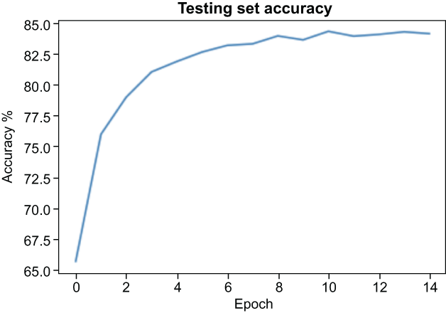
Figure 6.12 Fine-tuning VGG-11 peaked around 84% accuracy in the test set.
6.4.3 Using fine-tuned VGG-11 features with logistic regression
Our fine-tuning process was a great success, but we have one minor issue. We didn’t use a logistic regression to do the actual classification. We relied on the final feedforward layer in the classification section of the VGG-11 model to perform the actual classification, so we don’t know how much of the near-85% accuracy we achieved was due to the eight image representation layers learning better image representations and how much of it was due to the three classifier layers learning the best weights for classification. But we know how to tell!
Let’s take one more step to get accuracy results from our fine-tuned VGG-11 feature extractor and use logistic regression to perform the actual classification. Put another way, we will use the features section of our fine-tuned VGG-11 model to convert our raw images to features, and instead of using the classifier on the VGG-11, we will rely on the same logistic regression model we have been using for the other models. This will give us a good sense of how much better the VGG-11 features are compared to our other image vectorizers.
To do this, let’s load another VGG-11 model with the best weights from the training loop and rely on our helper function again to transform our standardized images in listing 6.16.
NOTE We could have used the model we just fine-tuned, but this is a good example of loading weights from a past training loop, and it is common practice to run accuracy metrics far after the training loop is complete.
Listing 6.16 Using a fine-tuned VGG-11 to extract features
cifar_fine_tuned_vgg_model = models.vgg11(                     ❶
    pretrained='imagenet')                                     ❶
cifar_fine_tuned_vgg_model.classifier[-1]                      ❶
.out_features = 10                                             ❶

cifar_fine_tuned_vgg_model.load_state_dict(
    torch.load('vgg_cifar10.pt',
map_location=device))                                          ❷

cifar_finetuned_training_images,
shuffled_training_labels,
cifar_finetuned_testing_images,
shuffled_testing_labels = get_vgg_features(
    cifar_fine_tuned_vgg_model.features)                       ❷

print("Fine-tuned VGG11 + LogReg
=====================")
advanced_grid_search(                                          ❸
    cifar_finetuned_training_images, shuffled_training_labels,
    cifar_finetuned_testing_images, shuffled_testing_labels,
    ml_pipeline, params
)
❶ Instantiate a new VGG-11 model.
❷ Load up the trained parameters, and extract fine-tuned features.
❸ Run a grid search on fine-tuned features.
Our results are nearly only 1% worse (figure 6.13) than the best testing accuracy we got during our training loop. This proves that our fine-tuning process really did lead to the VGG-11 model learning an optimal image representation for our CIFAR-10 dataset and was not simply relying on the classifier layer to achieve such a high performance.

Figure 6.13 A jump from 69% accuracy with the pretrained VGG-11 to 83% accuracy using the fine-tuned VGG-11 features proves that our fine-tuning method forced the VGG-11 model to learn an optimal representation of images for this particular object recognition task.
6.5 Image vectorization recap
We’ve seen many ways to vectorize images for ML pipelines in this chapter. Table 6.1 recaps each methodology, alongside their respective metrics. It’s clear that our transfer learning approach provided the best results, just as they did in the previous chapter on NLP.
For our images, however, the boost in performance is much sharper. This is likely because, well, a picture is worth 1,000 words. There is so much more variance and noise in images than in short tweets. This is likely why the delta in performance between CountVectorizers and BERT was not as dramatic as the difference between HOG features and VGG-11. As always, the vectorization method we choose to use for our unstructured text and images depends on the complexity of the data and the ML task.
Table 6.1 Showcasing our image vectorization methods with accompanying statistics. Overall, using VGG-11 with the feedforward network as a classifier yielded the best accuracy on our test set.
6.6 Answers to exercises
Find the cumulative percent of explained variance, using 10, 100, 200, and 400 principal components.
explained_variance = p.explained_variance_ratio_.cumsum()

for i in [10, 100, 200, 400]:
    print(f'The explained variance using {i}
    components is {explained_variance[i - 1]}')
The explained variance using 10 components is 0.17027868448637712
The explained variance using 100 components is 0.5219347292907045
The explained variance using 200 components is 0.696400699801984
The explained variance using 400 components is 0.9156784465873314Continue training the model for another three epochs, and calculate the change in testing accuracy.
Answers may vary here, due to the randomness involved with deep learning training.
Summary
-
Image vectorization and text vectorization are both ways of converting raw unstructured data into structured, fixed-length feature vectors, which are required for ML.
-
Feature construction and extraction techniques, like MPV and HOG, provide a great and fast baseline method for image vectorization but will generally fall short compared to longer, more complex deep learning techniques.