
Chapter 1
Prepare the data
Over the past several years, Microsoft Power BI has evolved from a new entrant in the data space to one of the most popular business intelligence tools used to visualize and analyze data. Before you can analyze data in Power BI, you need to prepare, model, and visualize the data. Data preparation is the subject of this chapter; we review the skills necessary to consume data in Power BI Desktop.
We start with the steps required to connect to various data sources. We then review the data profiling techniques, which help you “feel” the data. Later, we look at how you can clean and transform data by using Power Query—this activity often takes a disproportionate amount of time in many data analysis projects. Finally, we show how you can resolve data import errors after loading data.
Skills covered in this chapter:
Skill 1.1: Get data from different data sources
No matter what your data source is, you need to get data in Power BI before you can work with it. Power BI can connect to a wide variety of data sources, and the number of supported data sources grows every month. Furthermore, Power BI allows you to create your own connectors, making it possible to connect to virtually any data source.
The data consumption process begins with an understanding of business requirements and data sources available to you. For instance, if you need to work with near-real-time data, your data consumption process is going to be different compared to working with data that is going to be periodically refreshed. As you’ll see later in the chapter, different data sources support different connectivity modes.
Identify and connect to a data source
There are over 100 native connectors in Power BI Desktop, and the Power BI team is regularly making new connectors available. When connecting to data in Power BI, the most common data sources are files, databases, and web services.
Need More Review? Data Sources In Power BI
The full list of data sources available in Power BI can be found at https://docs.microsoft.com/en-us/power-bi/connect-data/power-bi-data-sources.
To choose the right connector, you must know what your data sources are. For example, you cannot use the Oracle database connector to connect to a SQL Server database, even though both are database connectors.
Note Companion Files
In our examples, we are going to use this book’s companion files, which are based on a fictitious company called Wide World Importers. Subsequent instructions assume that you placed all companion files in the C:PL-300 folder.
To review the skills needed to get data from different data sources, let’s start by connecting to the WideWorldImporters.xlsx file from this book’s companion files:
On the Home tab, select Excel workbook.
In the Open window, navigate to the WideWorldImporters.xlsx file and select Open.
In the Navigator window, select all eight check boxes on the left; the window should look similar to Figure 1-1.
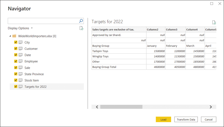
FIGURE 1-1 The Navigator window
Select Transform Data.
After you complete these steps, the Power Query Editor window opens automatically; you can see it in Figure 1-2.

FIGURE 1-2 Power Query Editor
If in the Navigator window you chose Load, the Power Query Editor window would not open, and all Excel sheets you selected would be loaded as is.
Note that the Navigator window shows you a preview of the objects you selected. For example, in Figure 1-1 we see the preview of the Targets for 2022 sheet; its shape suggests we need to apply some transformations to our data before loading it, because it has some extraneous information in its first few rows.
Note Data Preview Recentness
To make query editing experience more fluid, Power Query caches data previews. Therefore, if your data changes often, you may not see the latest data in Power Query Editor. To refresh a preview, you can select Home > Refresh Preview. To refresh previews of all queries, you should select Home > Refresh Preview > Refresh All.
The Navigator window is not unique to the Excel connector; indeed, you will see the same window when connecting to a complex data source like a database, for instance.
We are going to transform our data later in this chapter. Before we do that, let’s connect to another data source: a folder. While you are in Power Query Editor:
On the Home tab, select New Source. If you select the button label instead of the button, select More.
In the Get data window, select Folder and then Connect.
Select Browse, navigate to C:PL-300Targets, and select OK twice. At this stage, you should see the list of files in the folder like in Figure 1-3.

FIGURE 1-3 List of files in C:PL-300Targets
Select Combine & Transform Data.
In the Combine Files window, select OK without changing any settings.
At this stage, you have connected to two data sources: an Excel file and a folder, which contained several comma-separated values (CSV) files.
Although we did not specify the file type when connecting to a folder, Power Query automatically determined the type of files and applied the transformations it deemed appropriate. In addition to Excel and CSV files, Power BI can connect to several other file types, including JSON, XML, PDF, and Access database.
Important Format Consistency
It is important that the format of the files in a folder be consistent—otherwise, you may run into issues. Power Query applies the same transformations to each file in a folder, and it decides which transformations are necessary based on the sample file you choose in the Combine Files window.
Power Query Editor
If you followed our instructions, your Power Query Editor window should look like Figure 1-4.

FIGURE 1-4 Power Query Editor after connecting to Excel and a folder
As you can see, after you instructed Power Query to automatically combine files from the folder, it created the Targets query and several helper queries, whose names are italicized—this means they won’t be loaded. We will review the data loading options later in this chapter, and we’ll continue using the same queries we created in this example.
Note Companion Files
You can review the steps we took by opening the file 1.1.1 Connect.pbix from the companion files folder.
Query dependencies
You can check the dependencies queries have by selecting Query Dependencies on the View tab. The Query Dependencies view provides a diagram like the one in Figure 1-5 that shows both data sources and queries.

FIGURE 1-5 Query Dependencies view
To view the dependencies of a specific query, select a query, and Power BI will highlight both the queries that depend on the selected query as well as queries and sources that the query depends on.
The default layout is top to bottom; you can change the layout by using the Layout drop-down list.
Change data source settings
After you connect to a data source, sometimes you may need to change some settings associated with it. For example, if you moved the WideWorldImporters.xlsx file to a different folder, you’d need to update the file path in Power BI to continue working with it.
One way to change the data source settings is to select the cog wheel next to the Source step under Applied Steps in Query Settings in Power Query Editor. After you select the cog wheel, you can change the file path as well as the file type. The shortcoming of this approach is that you will need to change settings in each query that references the file, which can be tedious and error-prone if you have a lot of queries.
Another way to change the data source settings is by selecting Data source settings on the Home tab. This opens the Data source settings window, shown in Figure 1-6.

FIGURE 1-6 The Data source settings window
The Data source settings window allows you to change the source settings for all affected queries at the same time by selecting Change Source. You can change and clear the permissions for each data source by selecting Edit Permissions and Clear Permissions, respectively. Permissions include the credentials used for connecting to a data source and the privacy level. Privacy levels are relevant when combining data from different sources in a single query, and we will look at them later in this chapter.
Select a shared dataset or create a local dataset
So far in this chapter, we have been creating our own dataset, which is also known as a local dataset. If a dataset already exists that you or someone else prepared and published to the Power BI service, you can connect to that dataset, also known as a shared dataset. Using a shared dataset has several benefits:
You ensure consistent data across different reports.
When connecting to a shared dataset, you are not copying any data needlessly.
You can create a copy of an existing report and modify it, which takes less effort than starting from scratch.
Note Using Shared Datasets
Sometimes different teams want to see the same data by using different visuals. In that case, it makes sense to create a single dataset and different reports that all connect to the same dataset.
To be able to connect to a published dataset, you must have the Build permission or be a contributing member of the workspace where the dataset resides. We will review permissions in Chapter 4, “Deploy and maintain assets.”
You can connect to a shared dataset from either Power BI Desktop or the Power BI service:
In Power BI Desktop, select Power BI datasets on the Home tab.
In the Power BI service, when you are in a workspace, select New > Report > Pick a published dataset.
Either way, you will then see a list of shared datasets you can connect to, as shown in Figure 1-7. Additionally, in the Power BI service, you can select Save a copy next to a report in a workspace to create a copy of the report without duplicating the dataset. This will be similar to connecting to a dataset from Power BI Desktop because you will be creating a report without an underlying data model.

FIGURE 1-7 List of available datasets
After you are connected to a shared dataset in Power BI Desktop, some user interface buttons will be grayed out or missing because this connectivity mode comes with limitations. For example, when you connect to a shared dataset, Power Query Editor is not available, and the Data view is missing. In the lower-right corner, you’ll see the name and workspace you’re connected to, as shown in Figure 1-8.

FIGURE 1-8 Power BI Desktop connected to a Power BI dataset
You can select Transform Data > Data source settings to change the dataset you are connected to. You can also select Transform Data or Make changes to this model in the lower-right corner to create a composite model, where you can combine data from the shared dataset with other data. Composite models are covered in the “Select a storage mode” section.
If you choose not to create a composite model, note that you can still create measures, and they will be saved in your PBIX file but not in the shared dataset itself. That means other users who connect to the same shared dataset will not see the measures you created. These measures are known as local or report-level measures. Creating measures in general is going to be reviewed in Chapter 2, “Model the data.”
Select a storage mode
The most common way to consume data in Power BI is to import it into the data model. When you import data in Power BI, you create a copy of it that is kept static until you refresh your dataset. Data from files and folders, which we connected to earlier in the chapter, can be imported only in Power BI. When it comes to databases, you can create data connections in one of two ways.
First, you can import your data, which makes the Power BI data model cache it. This method offers you the greatest flexibility when you model your data because you can use all the available modeling features in Power BI.
Second, you can connect to your data directly in its original source. This method is known as DirectQuery. With DirectQuery, data is not cached in Power BI. Instead, the original data source is queried every time you interact with Power BI visuals. Not all data sources support DirectQuery.
A special case of DirectQuery called Live Connection exists for Analysis Services (both Tabular and Multidimensional) and the Power BI service. This connectivity mode ensures that all calculations take place in the corresponding data model.
Importing data
When you import data, you load a copy of it into Power BI. Since Power BI is based on an in-memory columnar database engine, the imported data consumes both the RAM and disk space, because data is stored in files. During the development phase, the imported data consumes the disk space and RAM of your development machine. After you publish your report to a server, the imported data consumes the disk space and RAM of the server to which you publish your report. The implication of this is that you can’t load more data into Power BI than your hardware allows. This becomes an issue when you work with very large volumes of data.
You have an option to transform data when you import it in Power BI, limited only by the functionality of Power BI. If you only load a subset of tables from your database, and you apply filters to some of the tables, only the filtered data gets loaded into Power BI.
After data is loaded into the Power BI cache, it is kept in a compressed state, thanks to the in-memory database engine. The compression depends on many factors, including data type, values, and cardinality of the columns. In most cases, however, data will take much less space once it is loaded into Power BI compared to its original size.
One of the advantages of this data connection method is that you can use all the functionality of Power BI without restrictions, including all transformations available in Power Query Editor, as well as all DAX functions when you model your data.
Additionally, you can combine imported data from more than one source in the same data model. For example, you can combine some data from a database and some data from an Excel file in a single table.
Another advantage of this method is the speed of calculations. Because the Power BI engine stores data in-memory in compressed state, there is little to no latency when accessing the data. Additionally, the engine is optimized for calculations, resulting in the best computing speed.
Data from imported tables can be seen in the Data view in Power BI Desktop, and you can see the relationships between tables in the Model view. The Report, Data, and Model buttons are shown in Figure 1-9 on the left.

FIGURE 1-9 Power BI Desktop when importing data
DirectQuery
When you use the DirectQuery connectivity mode, you are not caching any data in Power BI. All data remains in the data source, except for metadata, which Power BI caches. Metadata includes column and table names, data types, and relationships.
For most data sources supporting DirectQuery, when connecting to a data source, you select the entities you want to connect to, such as tables or views. Each entity becomes a table in your data model. The experience is similar to the Navigator window you saw earlier in the chapter when connecting to an Excel file, shown in Figure 1-1.
If you only use DirectQuery in your data model, the Power BI file size will be negligible compared to a file with imported data.
The main advantage of this method is that you are not limited by the hardware of your development machine or the capacity of the server to which you will publish your report. All data is kept in the data source, and all the calculations are done in the source as well.
Data from DirectQuery tables cannot be seen in the Data view of Power BI Desktop; if all tables in a data model are in DirectQuery mode, the Data view button will not be visible, though you can still use the Model view. A fragment of the interface when using DirectQuery is shown in Figure 1-10.

FIGURE 1-10 Power BI Desktop interface when using DirectQuery
Live Connection
A special case of DirectQuery, called Live Connection, is available for Power BI service datasets and Analysis Services data models. It differs from DirectQuery in a few ways:
You cannot apply any transformations to data.
It is not possible to define physical relationships in Live Connection.
Data modeling is limited to only creating measures.
You may consider using Live Connection rather than importing data because of the enhanced data modeling capabilities and improved security features in the data source. More specifically, unlike DirectQuery with some databases, Live Connection always considers the username of the user who is viewing a report, which means security can be set up dynamically. Additionally, SQL Server Analysis Services can be configured to refresh as frequently as needed, unlike the scheduled refresh in the Power BI service, which is limited to eight times a day without Power BI Premium.
If you connect to a dataset in DirectQuery or Live Connection mode and add other data, you’ll create a composite model, covered next.
Composite models
A composite model is a data model that combines imported data and DirectQuery or Live Connection data or that uses DirectQuery to connect to multiple data sources. For example, you could be getting the latest sales data from a database by using DirectQuery, and you could be importing an Excel spreadsheet with sales targets. You can combine both data sources in a single data model by creating a composite model.
Important Potential Security Risks In Composite Models
Building a composite model may pose security risks; for example, data from an Excel file may be sent to a database in a query, and a database administrator might see some data from the Excel file.
For each table in a composite model that uses imported data or DirectQuery, the storage mode property defines how the table is stored in the data model. To view the property, you can hover over a table in the Fields pane in the Report or Data view; alternatively, you can view or change it in the Model view in the Advanced section of the Properties pane once you select a table. Note that you cannot change the storage mode of tables that you get from models by using Live Connection.
Storage mode can be set to one of the following options:
Import
DirectQuery
Dual
The Dual mode means a table is both cached and retrieved in DirectQuery mode when needed, depending on the storage mode of other tables used in the same query. This mode is useful whenever you have a table that is related to some imported tables and other tables whose storage mode is DirectQuery. For example, consider the data model from Table 1-1.
TABLE 1-1 Sample data model
Table Name | Data Source | Storage Mode |
|---|---|---|
Sales | Database | DirectQuery |
Date | Database | Dual |
Targets | Excel file | Import |
In this model, the Date table is related to both the Sales and the Targets tables. When you use data from the Date and Sales tables, it is retrieved directly from the database in DirectQuery mode; when you use Date and Targets together, no query is sent to the database, which improves the performance of your reports.
Important Changing Storage Mode
If you change the storage mode from DirectQuery or Dual to Import, there is no going back. If you need to set the storage mode of a table to Dual, you must create a table by using DirectQuery first.
Use Microsoft Dataverse
Power Platform has a family of products that offer similar experiences when you get data in Power BI:
Dataflows
Microsoft Dataverse (formerly known as Common Data Service)
Both Dataflows and Microsoft Dataverse store data in tables, also known as entities. Dataverse also offers a set of standardized tables that you can map your data to, or you can create your own tables.
Connecting to Dataflows only requires you to sign in, and then you’ll see the dataflows and tables you have access to.
To connect to Microsoft Dataverse, you’ll need to know the server address, which usually has the following format: environment.crm.dynamics.com.
Need More Review? Finding Server Addresses
If you want to learn how to find the server name, see the step-by-step tutorial here: https://docs.microsoft.com/en-us/powerapps/maker/data-platform/data-platformpowerbi-connector.
Additionally, you’ll need maker permissions to access the Power Apps portal and read permissions to access data within entities. Afterward, the connection experience is similar to connecting to a database.
Change the value in a parameter
Query parameters can simplify certain tasks, like changing a data source address or placing a filter in a query. Here are some examples of when you’d use parameters:
Switching between the development and production environments when getting data from a database
Configuring incremental refresh (outside of the scope of this book)
Creating custom functions by using the user interface
Using report templates
Need More Review? Templates In Power BI Desktop
Power BI report templates can be used as a starting point when you analyze data in Power BI. Power BI report templates are out of the scope of this book. More information on how you can create and use report templates is available at https://docs.microsoft.com/en-us/power-bi/create-reports/desktop-templates.
Creating parameters
To create a new parameter in Power Query Editor, on the Home ribbon select Manage Parameters > New Parameter. You will then see the Manage Parameters window shown in Figure 1-11.

FIGURE 1-11 The Manage Parameters window
For each parameter, you can configure the following options:
Name This will become the parameter name by which you can reference it.
Description This will show up when you hover over the parameter in the Queries pane or when you open a report template that contains the parameter.
Required This determines whether the parameter value can be empty.
Type This is the data type of the parameter. Not all Power Query data types are available. For example, whole number cannot be selected; instead, you can choose decimal number for numerical parameters.
Suggested Values You can choose one of these three options:
Any value This is the default setting, and it allows any value within the limits of the parameter type.
List of values This allows you to type a list of values from which you can choose a parameter. When you use this option, you may also specify the default value, which will be selected if you open a template with this parameter.
Query When this option is selected, you will need to use a query of type list that will feed the list of values.
Current Value This is the value the parameter returns when you reference it.
Important Parameter Type
If you intend to change a parameter in the Power BI service, you must set its data type correctly. Using the Any type will prevent you from editing the parameter value in the Power BI service.
Using parameters
Let’s follow an example of how to use parameters in practice:
Create a new Power BI Desktop file.
Open Power Query Editor by selecting Transform data on the Home ribbon.
Create a new parameter as follows:
Name: Year
Type: Decimal number
Current Value: 2006
Leave all other parameter options as is and select OK.
Now that you have created the new parameter, let’s connect to the CompanySales table from the AdventureWorks OData feed:
Still in Power Query Editor, select New Source > OData feed.
Enter https://services.odata.org/AdventureWorksV3/AdventureWorks.svc/ in the URL box and select OK. If prompted for credentials, select Anonymous.
Select the CompanySales check box and select OK.
In the lower-left corner of Power Query Editor, note that the CompanySales query, which you’ve just created, returns 235 rows. We are now going to use our parameter to filter the query as follows:
Select the filter button on the OrderYear column header and select Number Filters > Equals. You will be presented with the filter options in Figure 1-12.

FIGURE 1-12 Filter rows options
Select the top 1.2 drop-down list next to equals and select Parameter. Note that the Year parameter we created earlier is automatically selected because it is the only parameter.
Select OK.
The query now returns 50 rows, because it is filtered to only show rows where OrderYear is 2006—the current value of the Year parameter.
Editing parameters
You can edit parameters in Power BI Desktop or the Power BI service. Editing a parameter refers to changing its current value, as opposed to managing a parameter, which refers to changing any parameter attribute.
To continue with our example, you can edit the Year parameter by selecting it in the Queries pane and changing its current value to 2007. Note how the CompanySales query now returns 96 rows instead of 50.
Note Companion Files
You can review this example by opening 1.1.6 Parameters.pbix from the companion files folder.
Note Editing Multiple Parameters
If you had several parameters, it would be more convenient to edit all the parameters at once. In the main Power BI Desktop window, you can select Transform data > Edit parameters; alternatively, in Power Query Editor, select Manage Parameters > Edit Parameters.
You can also edit parameters after publishing your report to the Power BI service. This is done in the Parameters section of dataset settings, as shown in Figure 1-13.

FIGURE 1-13 Editing parameters in the Power BI service
After you change the parameter value, select Apply.
Need More Review? Power BI Service
We review the Power BI service in more detail in Chapter 4.
Creating functions
Power Query allows you to create your own functions, which can be useful when you want to apply the same logic multiple times. One way to create a custom function is by converting a query to a function. If your query already uses parameters, then those will become the parameters of the new function.
Let’s continue our AdventureWorks example and create a function that will output sales for a particular year based on the year you enter:
Right-click the CompanySales query and select Create Function.
In the Function name box, enter SalesByYear.
Select OK.
This creates the SalesByYear group of queries, which contains the Year parameter, the CompanySales query, and the SalesByYear function.
Now test the new function:
Select the SalesByYear function in the Queries pane.
Enter 2008 in the Year box.
Select Invoke.
This creates the Invoked Function query that returns 73 rows and contains data for year 2008 only, which you can verify by selecting the OrderYear column filter button.
Note that there is a special relationship between the SalesByYear function and CompanySales query: updating the latter also updates the former, which in turn updates all function invocations. For example, we can remove the ID column from the CompanySales query, and it will disappear from the Invoked Function query, too.
 Exam Tip
You should be able to identify scenarios when query parameters can be beneficial based on the business requirements of a client.
Connect to a dataflow
In addition to Power BI Desktop, Power Query can be found in the Power BI service: you can prep, clean, and transform data in dataflows. Dataflows can be useful when you want your Power Query queries to be reused across your organization without the queries necessarily being in the same dataset. For this reason, you cannot create a dataflow in your own workspace, because only you have access to it.
To create a dataflow in a workspace, select New > Dataflow. From there, you have several choices:
Add new tables Define new tables from scratch by using Power Query.
Add linked tables Linked entities are tables in other dataflows that you can reuse to reduce duplication of data and improve consistency across your organization.
Import model If you have a previously exported dataflow model file, you can import it.
Create and attach Attach a Common Data Model folder from your Azure Data Lake Storage Gen2 account and use it in Power BI.
The Power Query Online interface (Figure 1-14) looks similar to Power Query Editor in Power BI Desktop.

FIGURE 1-14 Power Query interface when editing a dataflow
Once you finish authoring your queries, you can select Save & close and enter the name of the new dataflow. After saving, you’ll need to refresh the dataflow by selecting Refresh now from the dataflow options in the workspace—otherwise, it won’t contain any data. When a dataflow finishes refreshing, you can connect to it from Power BI Desktop and get data from it.
Skill 1.2: Clean, transform, and load the data
Unless you are connecting to a dataset that someone has already prepared for you, in many cases you must clean and transform data before you can load and analyze it.
Power BI contains a powerful ETL (extract, transform, load) tool: Power Query. Power Query, also known as Get & Transform Data, first appeared as an add-in for Excel 2010; starting with Excel 2016, it has been an integral part of Excel. You can see Power Query in several other Microsoft products, including Power Apps and Power Automate.
When you connected to various data sources and worked inside Power Query Editor earlier in this chapter, you were using Power Query. Besides connecting to data, Power Query can perform sophisticated transformations to your data. In this book, Power Query refers to the engine behind Power Query Editor.
Power Query uses a programming language called M, which is short for “mashup.” It is a functional, case-sensitive language. The latter point is worth noting because M is case-sensitive, unlike the other language of Power BI we are going to cover later, DAX. In addition, M is a completely new language that, unlike DAX, does not resemble Excel formula language in any way.
This skill covers how to:
Profile the data
Resolve inconsistencies, unexpected or null values, and data quality issues
Identify and create appropriate keys for joins
Evaluate and transform column data types
Shape and transform tables
Combine queries
Apply user-friendly naming conventions to columns and queries
Configure data loading
Resolve data import errors
Profile the data
When performing data analysis, you will find it useful to see the overall structure or shape of data, which you can achieve by profiling data. Data profiling allows you to describe its content and consistency. It’s advisable to do data profiling before working with data, because you can discover limitations in the source data and then decide if a better data source would be required. If you analyze the data without profiling it, you may miss outliers, and your results may not be representative of what’s really happening.
Power Query has column profiling capabilities that can be used to profile your data before you even load it. These include column quality, column value distribution, and column profile.
Identify data anomalies
Power Query provides different functionality for identifying data anomalies depending on what you are looking for; you might be looking for unexpected values, such as prices over $10,000 when you analyze sales of a retail store, or you may be looking for missing or error values. In this section, we cover missing or error values, and later in the chapter we look at how you can identify unexpected values.
When you look at a table in Power Query Editor, you can check the quality of each column. By default, each column will have a colored bar under its header, which shows how many valid, error, and empty values there are in each column. To show the exact percentages, select View > Data Preview > Column quality.
Note Companion Files
Open 1.1.1 Connect.pbix from the companion files folder to follow along with the examples.
Figure 1-15 shows the Employee query from our earlier Wide World Importers example with the Column quality feature enabled.

FIGURE 1-15 Column quality
Note how the Parent Employee Key column has 85% valid values and 15% empty ones. If we didn’t expect any empty values in the column, this would prompt us to investigate the issue. For the column quality purposes in Power Query, empty values are null values or empty strings. There are no errors in this query, so the Error percentage is always 0%.
If we now go to the Customer query and check the Postal Code column, we’ll see that there are <1% error values. Note that Power Query won’t tell you the percentage of valid or missing values when there are errors in a column. For now, we’ll leave this error as is, and we’re going to fix the error in this column later in this chapter.
To copy the column quality metrics, right-click the area under the column header and select Copy Quality Metrics.
Important Data Sample
By default, column profiling is based on the first 1,000 rows of a query. You can use the entire dataset for column profiling by making a change in the lower-left corner of Power Query Editor.
Examine data structures and interrogate column properties
In addition to column quality, you can look at column value distribution. To enable this feature, select View > Data Preview > Column distribution. In Figure 1-16, you can see the Stock Item query with this feature enabled.

FIGURE 1-16 Column distribution
Note that you can now see how many distinct and unique values each column has, as well as the distribution of column values in the form of a column chart under each column header. Column profiling is shown irrespective of the column type, which you can see to the left of a column’s name.
The distinct number refers to how many different values there are in a column once duplicates are excluded. The unique number shows how many values occur exactly once. The number of distinct and unique values will be the same only if all values are unique.
The column charts show the shape of the data—you can see whether the distribution of values is uniform or if some values appear more frequently than others. For example, in Figure 1-16, you can see that the Selling Package column mostly consists of one value, with four other values appearing significantly less frequently.
To copy the data behind a column chart, right-click a column chart and select Copy Value Distribution. This will provide you with a list of distinct values and the number of times they appear in the column.
Knowing the column distribution can be particularly useful to identify columns that don’t add value to your analysis. For example, in the State Province query, you can see that the following columns have only one distinct value each:
Country
Continent
Region
Subregion
Depending on your circumstances, you may choose to remove the columns to declutter your queries.
Note Understanding Value Distribution
The distribution of values is based on the current query only. For example, the distribution of the Stock Item Key column values may be different in the Stock Item and Sale queries. It’s also worth remembering that the distribution of values may be different if you choose to profile the entire dataset as opposed to the first 1,000 rows.
Need More Review? Table Schema
You can see the advanced properties of columns, such as their numeric precision or whether they are nullable, by using the Table.Schema function. Writing your own M code is outside the scope of this book. For more information about the Table.Schema function, visit https://docs.microsoft.com/en-us/powerquery-m/table-schema.
Interrogate data statistics
You can also profile columns to get some statistics and better understand your data. To enable this feature, select View > Data Preview > Column profile. After you enable this feature, select a column header to see its profile. For example, Figure 1-17 shows the profile of the Unit Price column from the Stock Item query.

FIGURE 1-17 Column profile
You can now see two new areas in the lower part of Power Query Editor:
Column statistics This shows various statistics for the column. In addition to the total count of values and the number of error, empty, distinct, and unique values, you can see other statistics, such as minimum, maximum, average, and the number of zero, odd, and even values, among others. You will see different statistics depending on the column type. For instance, for text columns you will see the number of empty strings in addition to the number of empty values. You can copy the statistics by selecting the ellipsis next to Column statistics and selecting Copy.
Value distribution This is a more detailed version of the column chart you can see under the column name. You can now see which column refers to which value, and you can hover over a column to apply filters based on the corresponding value. You can copy the value distribution as text by selecting the ellipsis on the Value distribution header and selecting Copy. Also when you select the ellipsis, you can group the values depending on the data type. For example, you can group columns of type Date by year, month, day, week of year, and day of week. Text values can be grouped by text length. Whole numbers can be grouped by sign or parity (odd or even), whereas decimals can be grouped by sign only.
Need More Review? Profiling Tables
If you want to profile the whole table at once, you can use the Table.Profile function, which is not available when you are using the user interface alone, though you can write your own code to use it. For more information about the Table.Profile function, visit https://docs.microsoft.com/en-us/powerquery-m/table-profile.
Resolve inconsistencies, unexpected or null values, and data quality issues
If you followed the Wide World Importers example earlier in the chapter, you’d recall that the Postal Code column in the Customer query had an error in it. Power Query offers several ways to deal with errors or other unexpected values:
Replace values
Remove rows
Identify the root cause of error
Replace values
You can replace undesirable values with different values by using the Power Query user interface. This approach can be appropriate when there are error values in the data source that you cannot fix. For example, when connecting to Excel, the #N/A values will show up as errors. Unless you can fix the errors in the source, it may be acceptable to replace them with some other values.
Since errors are not values as such, the procedure to replace them is different compared to replacing other unexpected values.
To replace errors:
Right-click a column header and select Replace Errors.
Enter the value you want to replace errors with in the Value box.
Select OK.
You can only replace errors in one column at a time when using the user interface.
To replace a value in a column:
Right-click a column header and select Replace Values.
Enter the value you want to replace in the Value To Find box.
Enter the replacement value in the Replace With box.
Select OK.
You can also right-click a value in the column and select Replace Values. This way, the Value To Find box will be prepopulated with the selected value.
For text columns, you can use the advanced options shown in Figure 1-18.

FIGURE 1-18 Replace Values options
Match entire cell contents With this option checked, Power Query won’t replace values where the Replace With value is only part of the Value To Find value.
Replace using special characters Use this to insert special character codes, such as a carriage return or a nonbreaking space, in the Replace With or Value To Find box.
To replace values in multiple columns at once, you must select multiple columns before replacing values. To do so, hold the Ctrl key and select the columns whose values you want to replace. If you want to select a range of columns based on their order, you can select the first column, hold the Shift key, and select the last column.
The type of the replacement value must be compatible with the data type of the column—otherwise, you may get errors.
Note Null Values In Power Query
Null values are special values in Power Query. If you want to replace a value with a null, or vice versa, enter the word null in the relevant box, and Power Query will recognize it as a special value rather than text.
Remove rows
If there are errors in a column, you may wish to remove the rows entirely, depending on the business requirements. To do so, you can right-click a column header and select Remove Errors. Note that this will only remove rows where there are errors in the selected column. If you wish to remove all rows in a table that contain errors in any column, you can select the table icon to the left of the column headers and select Remove Errors.
Identify the root cause of error
When you see an error in a column, you can check the error message behind the error. To do so, select the error cell, and you will see the error message in the preview section at the bottom.
Note Checking the Cell Contents
In general, you can use this method—selecting the cell—to see nested cell contents such as errors, lists, records, and tables.
Though you also have an option to select the hyperlink, keep in mind that this will add an extra query step, which you will have to remove if you want to load the query later.
Figure 1-19 shows the error message behind the error we saw in the Postal Code column of the Customer query.

FIGURE 1-19 Error message
After seeing this error message, you know that the error happened because Power Query tried to convert N/A, which is text, into a number. To confirm this, you can go one step back by selecting the Promoted Headers step in the list of Applied Steps—the cell will show N/A, so you must transform the column type to Text to prevent the error from happening, as covered later in this chapter.
Although errors can happen for a variety of reasons, and not all errors occur because of type conversions, reading the error message will usually give you a good idea of what’s going on.
Identify and create appropriate keys for joins
Power BI allows you to combine data from different tables in several ways. Most commonly, you combine tables, or you create relationships between them.
Combining tables requires a join in the query, which in Power Query is also known as merge. Relationships, which you create in the model, not in Power Query, create implicit joins when visuals calculate values. The choice between the two depends on the business requirements and is up to the data modeler. In this section, we are discussing the keys you need for either operation.
Need More Review? Combining Tables and Creating Relationships
We review different methods of combining tables later in this chapter, and we cover relationships in Chapter 2.
When you join tables, you need to have some criteria to join them, such as keys in each table. For example, you join the City and Sale tables by using the City Key column in each table. Though it’s handy to have keys named in the same way, it’s not required. For instance, you can join the Sale table with the Date table by using the Invoice Date Key from the Sale table and the Date column from the Date table.
Each table can be on the one or the many side during a join. If a table is on the one side, it means the key in the table has a unique value for every row, and it’s also known as the primary key. If a table is on the many side, it means that values in the key column are not necessarily unique for every row and may repeat, and such a key is often called a foreign key.
You can join tables that are both on the one side, but such situations are rare. Usually one table is on the one side and one table is on the many side. You can also perform joins when both tables are on the many side, though you should be aware that if you do it in Power Query, you will get duplicate rows.
Keys for joins in Power Query
Power Query allows you to perform joins based on one or more columns at once, so it’s not necessary to create composite keys to merge tables in Power Query.
For joins in Power Query, column types are important. For example, if a column is of type Date, then you won’t be able to merge it with a column of type Date/Time even if the Date/Time column has no Time component.
Keys for relationships
For relationships, Power BI is more forgiving of the data type. If columns that participate in a relationship are of different types, Power BI will do its best to convert them in one type behind the scenes. Although the relationship may still work, it’s always best to have the same data type for columns that are in a relationship.
Power BI only allows you to create physical relationships between two tables on a single pair of columns. This means that in case you have a composite key in a table, you’ll need to combine the key columns in a single column before you can create a physical relationship between two tables. You can do it in Power Query or by creating a calculated column in DAX.
Need More Review? Calculated Columns and Dax
If you use DirectQuery, some calculated columns can still be translated into the native language of the data source efficiently. For example, the COMBINEVALUES function in DAX translates well into SQL. We review DAX in Chapter 2.
There are two ways of combining columns in Power Query:
Create a new column This option keeps the original columns. To add a new merged column, select the columns you want to combine and select Add column > From Text > Merge Columns.
Merge columns in-place This option removes the original columns. To merge existing columns, select the columns you want to merge and select Transform > Text Column > Merge Columns.
Important Column Selection Order
The order in which you select columns matters: the order of the text in the merged column follows the order of column selection. In other words, if you select column A first and then column B, the result will be different compared to your selecting column B first and then column A.
Either way, you’ll be presented with the options shown in Figure 1-20.

FIGURE 1-20 Merge columns options
You can use one of the predefined separators from the Separator drop-down list, or you can specify your own by selecting Custom from the drop-down list. You’re also given an option to enter the new column name. After you specify the options, select OK.
Evaluate and transform column data types
If the data source does not communicate the type of each column, by default Power Query will do its best to detect the data types automatically if types are not available. So, for example, you’ll get column types from a database but not from a JSON file, so Power Query will try to detect types. It’s important to note that the process is not perfect because Power Query does not always consider all values. As you saw earlier, Power Query may detect data types incorrectly.
Note Disabling Automatic Type Detection
If you find the automatic type detection undesirable, you can turn it off at File > Options and settings > Options > Current file > Data Load > Type Detection.
Power Query supports the following data types:
Decimal Number
Fixed Decimal Number
Whole Number
Percentage
Date/Time
Date
Time
Date/Time/Timezone
Duration
Text
True/False
Binary
Note Complex Data Types
Sometimes you may see other—complex—data types, like Function, List, Record, and Table. You will encounter some of them later in this chapter.
It’s also important to note that not all data types are available once you load your data. For example, the Percentage type becomes Decimal Number. We are reviewing data loading toward the end of this chapter.
Need More Review? Data Types In Power BI
Not all values can be stored in Power BI. For technical documentation on the data types in Power BI, including the supported range of values, visit https://docs.microsoft.com/en-us/power-bi/connect-data/desktop-data-types.
Continuing our Wide World Importers example, we now know that there is an error in the Postal Code column of the Customer query due to data type conversion. Power Query scanned the first few rows and, seeing whole numbers, decided that the type of the column is Whole Number, which you can see from the icon on the left side of the column header.
In our example, you should transform the Postal Code column type to Text to accommodate both numeric and text values.
Note Selecting the Data Type
Occasionally, selecting the data type may not be straightforward. For example, the calendar year number can be both numeric and text, but it is up to the data modeler to decide what the type should be.
In general, if it doesn’t make sense to perform mathematical operations with a column, then you may want to make it Text. In the case of a calendar year number, you may want to use it to apply filter conditions such as “greater than,” so the Whole Number type makes sense. In other cases, like postal codes, you probably won’t need to perform mathematical operations, so the Text type might be appropriate.
To transform the column type, right-click a column header, then select Change Type and select the desired data type. Alternatively, you can select the column type icon on the column header, and then select the data type you want to transform the column to.
Provided the last step in the Customer query is Changed Type and the step is selected, after you try to change the type of the Postal Code column, you will see the message shown in Figure 1-21.

FIGURE 1-21 Change Column Type dialog box
Since Power Query has already automatically changed the type of the column before, you now have the option to either replace the conversion by selecting Replace current or add a new conversion on top of the existing one by selecting Add new step.
In this case, you should replace the current conversion because otherwise Power Query will try to convert the error value to Text, and it will still be an error. After you select Replace current, you will not see any errors, and you will be able to see the column distribution and other statistics.
Note Caching In Power Query
If you still see errors after transforming type to Text, you should navigate to another query and come back to Customer. This is because Power Query sometimes caches the output and does not immediately update it.
Adding a new conversion step is appropriate in case you cannot convert the type in one step. For example, if you’ve got data in a CSV file, and there’s a column that contains Date/Time values, you will not be able to set the column type to Date. Instead, you should set the data type to Date/Time first, and then add a new conversion step that changes the type to Date. This way, you will get no errors.
If you want Power Query to detect the type of one or more specific columns automatically, you can select the columns, then select Transform > Any Column > Detect Data Type.
Using locale
Occasionally, you will need to transform data by using a certain locale. For example, if your computer uses the DMY date format and you receive data in MDY format, you’ll need to change type with the locale. To do so, right-click a column header and select Change Type > Using Locale. From there, you’ll need to select the data type and locale from drop-down lists.
Note Dates and Locale
In some cases, like monthly data, selecting the incorrect locale may not result in errors, since 1–12 can be either 1 December or 12 January. Therefore, it is especially important to ensure your data comes in the expected format when the values can be ambiguous.
Shape and transform tables
Few data sources provide data in shapes that are ready to be used by Power BI. You’ll often need to transform your data, especially if you work with files. In this section, we review common table transformations in Power Query by transforming the Wide World Importers queries that contain sales targets: Targets for 2022 and Targets.
Note Companion Files
If you want to follow along with the example, use 1.1.1 Connect.pbix from the companion files folder.
In Figure 1-22, you can see the first four columns of the Targets for 2022 query. There are 14 columns and seven rows in this query, which you can check by looking at the lower-left corner of Power Query when viewing the query.

FIGURE 1-22 Targets for 2022
Note Query Row Count
The row count is based on the query preview, and it may not account for all rows. You’ll get a more accurate figure in the Data view after you load data.
As you can see, the Targets for 2022 query is not yet ready to be used in Power BI for the following reasons:
There are extraneous notes in the first few rows.
There are totals.
There is no date or month column.
Values are pivoted.
Data types are not set.
In Figure 1-23, you can see the Targets query.

FIGURE 1-23 Targets query
There are several issues with this query, too:
Targets are provided at year level, but we need them to be at month level.
Years come from filenames and have the .csv extension suffix.
Targets are in millions instead of dollars.
After you transform each query, you must combine them. In our example, we’re aiming for a single table with the following columns:
End of Month You’ll need to make a relationship with the Date table later, and you can use a column of type Date for that.
Buying Group Only three values and no totals.
Target Excluding Tax In dollars, for each month.
Working with query steps
To start getting the Targets for 2022 query in the right shape, let’s undo some of the automatic transformations done by Power Query. By looking at the Applied Steps pane, you can see that after navigating to the right sheet in the Excel file, Power Query has promoted the first row to headers, even though the row did not contain column names. It also changed column types, considering column names as valid column values, which led to incorrect data type selection.
Right-click the Promoted Headers step in the Applied Steps pane.
Select Delete Until End.
Select Delete.
This removes the Promoted Headers step and all subsequent steps. The Delete Until End option is especially useful when you have more than two steps you want to remove.
Important Editing Steps
You can remove a single query step by selecting the cross icon. To change the order of steps, you can drag and drop a step. Some steps will have a gear icon—this will allow you to change the step options, if available.
It’s important to note that the query may break if you edit intermediate steps, since the order of steps in a query is sequential and most steps reference the previous step. For example, if you promote the first row to headers first, then change the column types, and then change the order of the last two steps, your query will break because the Changed Type step will be referencing incorrect column names.
As Figure 1-24 shows, you can now see some notes left by a sales planner in the first two rows. Note that columns are now not typed.

FIGURE 1-24 Targets for 2022 with automatic transformations undone
Reducing rows and columns
Since the first three rows don’t contain any meaningful data, we can remove them. In addition to filtering columns, the Power Query user interface offers the following options for row reduction:
Keep Rows
Keep Top Rows Keeps the specified number of top rows. Works on the whole table only.
Keep Bottom Rows Keeps the specified number of bottom rows. Works on the whole table only.
Keep Range of Rows Skips a specified number of top rows and then keeps the chosen number of rows. Works on the whole table only.
Keep Duplicates Keeps rows that appear more than once. This option can work on the whole table, meaning all column values will have to match for rows to be considered duplicates, or it can work on selected columns only, so values will only need to match in specified columns for duplicates to be kept.
Keep Errors Keeps rows that contain errors. This option can work on the whole table or selected columns only.
Remove Rows
Remove Top Rows Removes a specified number of top rows. Works on the whole table only.
Remove Bottom Rows Removes a specified number of bottom rows. Works on the whole table only.
Remove Alternate Rows Removes rows following a user-supplied pattern: it starts with a specified row, then alternates between removing the selected number of rows and keeping the chosen number of rows. Works on the whole table only.
Remove Duplicates Removes rows that are duplicates of other rows. Can work on the whole table or selected columns only.
Remove Blank Rows Removes rows that completely consist of empty strings or nulls. Works on the whole table only; if you need to remove blank values from a specific column, you can select the filter button to the right of a column’s name and select Remove Empty.
Remove Errors Removes rows that contain errors. Can work on the whole table or selected columns only.
Since notes can potentially change, it’s best not to remove them by filtering out specific values. In our case, Remove Top Rows is appropriate, so we can perform the following steps:
Select Remove Rows on the Home ribbon.
Select Remove Top Rows.
Enter 3 in the Number of rows box.
Select OK.
Now that we have removed the top three rows, we can use the first row for the column names by selecting Use First Row as Headers on the Home ribbon. The result should look like Figure 1-25.

FIGURE 1-25 Targets for 2022 with unnecessary rows removed and headers in place
Note how Power Query automatically detected column types, this time correctly since only the first column is a text column and all the other columns are numeric.
Next, you can see that the last row is a total row, and the last column, Year Target, is a total column. You need to remove both, because keeping them may result in incorrect aggregation later in Power BI.
There are several ways to remove the last row, and which way is best for you depends on several factors:
If you’re sure that the last row is always going to be a total row, you can remove it in the same way that you removed the top three rows earlier.
If, on the other hand, you’re not sure that the total row is always going to be there, it’s safer to filter out a specific value from the Buying Group column—in our example, Buying Group Total.
Depending on business logic, you can also apply a text filter that excludes values that end with the word Total. This kind of filter relies on actual Buying Group column values not ending with Total.
Important Case Sensitivity In Power Query
Since Power Query is case-sensitive by default, you must exclude the word “Total”; filtering out “total” won’t work.
Let’s say you’re sure that only the total row label ends with the word Total, so we can apply a corresponding filter to the Buying Group column as follows:
Select the filter button on the Buying Group column header.
Select Text Filters > Does Not End With.
Enter Total in the box next to the drop-down list that shows does not end with.
Select OK.
The last row is now filtered out, and you should remove the last column as well, since it contains totals for the year. To do so, select the Year Target column and press the Delete key.
With the totals gone, Power Query Editor should show “13 columns, 3 rows” in the lower-left corner. However, the current Targets for 2022 query still does not meet our goals because we don’t have a single date or month column. Instead, targets for each month appear in a separate column. We’ll address this issue next.
Pivoting columns, unpivoting columns, and transposing
The current Targets for 2022 query is sometimes called pivoted because attributes appear on both rows and columns and the same measure is scattered across multiple columns—just like in an Excel PivotTable.
Power Query provides several options when it comes to pivoting and unpivoting:
Pivot Column This creates a new column for each value in the column you pivot. One scenario when this option can be useful is when you have different measures mixed in the same column. For example, if you have Quantity and Price as text labels in one column and numeric quantity and price values in another column, you could pivot the first column to create separate Quantity and Price columns with numeric quantity and price values, respectively.
Unpivot Columns The selected columns will be transformed into two: Attribute, containing old column names, and Value, containing old column values. In general, unpivoting is useful when the source data has been prepared by using a PivotTable or similar method. This specific option is appropriate when the list of columns you want to unpivot is known in advance.
Unpivot Other Columns All columns except the selected ones will be unpivoted. This option is particularly useful when you only know the list of columns that don’t need to be unpivoted. For example, if you have a file where monthly data is added as columns every month and you want to unpivot months, then you could use this option.
Unpivot Only Selected Columns Despite the names of the previous two options, Power Query tries to recognize when you want to unpivot the selected columns or other columns, so this option allows you to be strict about which columns are unpivoted.
Furthermore, Power Query offers the Transpose feature, which allows you to transpose tables, treating rows as columns and columns as rows. This operation can be useful when you have multiple levels of headers; you can transpose your table, merge the columns that contain headers, and transpose again, so there will be only one row of headers.
Important Table Transposition and Column Names
When transposing tables, remember that you lose column names during the operation, so if you want to keep them, you must demote headers to the first row. You can do so by selecting the Use First Row as Headers drop-down and then selecting Use Headers as First Row.
For our Wide World Importers example, right-click the Buying Group column and select Unpivot Other Columns. This puts all column headers except for Buying Group in a single column called Attribute, and it puts all values in the Value column. The result should look like Figure 1-26.

FIGURE 1-26 Unpivoted months
As you can see, months now appear in a single column, which is what we want for Power BI. Now you need to transform month names into date values so you can create a relationship with the Date table later.
Adding columns
You can add a new column in Power Query by using one of the following options on the Add column ribbon:
Column From Examples This option allows you to type some examples in a new column, and Power Query will try its best to write a transformation formula to accommodate the examples.
Custom Column You can type your own M formula for the new column.
Invoke Custom Function This option invokes a custom function for every row of a table.
Conditional Column This option provides an interface where you can specify the if-then-else logic for your new column.
Index Column This option creates a sequential column that starts and increments with the values you specify. By default, it will start with 0 and increment by 1 for each row.
Duplicate Column This option creates a copy of a column you select.
In addition to these options, you can use data type–specific transformations to add columns, most of which are also available on the Transform ribbon. The difference between the Add Column and Transform ribbons is that the former will add a new column whereas the latter will transform a column in place.
Targets For 2022
In the Targets for 2022 query, you must transform month names into dates, and you’ll use the Custom Column option for this as follows:
Select Add Column > Custom Column.
Enter Start of Month in the New column name box.
Enter Date.From([Attribute] & “2022”) in the Custom column formula box. The Custom Column window should look like Figure 1-27.

FIGURE 1-27 Custom Column window
Select OK.
Right-click the Attribute column and select Remove.
When entering a custom column formula, you can use the columns available in the table by double-clicking them in the Available columns list on the right; this will insert a column reference into your formula.
Once you complete these steps, the result should look like Figure 1-28.

FIGURE 1-28 Targets for 2022 with Start of Month column
Important Custom Column Types
The Custom column feature creates a column without a data type by default; you must set the data type manually before loading to ensure that the data is loaded correctly.
As you can see, the Start of Month column you’ve just created has no column type, and you may want to make it the first column instead of the last. Additionally, you have to rename the Value column by completing the following steps:
Select the ABC123 icon on the Start of Month column header and select Date.
Right-click the Start of Month column and select Move > To Beginning.
Double-click the Value column header.
Enter Target Excluding Tax and press the Enter key.
The Targets for 2022 query is now finished, and we need to transform the Targets query next.
Targets
In the Targets query, you have yearly targets, and you need to have monthly targets. Let’s say that, according to business rules, it’s all right to divide the yearly target evenly across months for years prior to 2022, which this query contains.
There are a few ways to solve this problem, one of which is adding a new column that contains months and expanding it as follows:
Select Add Column > Custom Column.
Enter Months in the New column name box.
Enter {1..12} in the Custom column formula box.
Select OK.
The result should look like Figure 1-29.

FIGURE 1-29 Months custom column added to the Targets query
In M, braces signify a list, and a double period signifies a range. When you used {1..12} as a custom column formula, you put a list of numbers from 1 to 12, inclusive, in each cell of the new column. Therefore, you see the List hyperlinks in the Months column cells. Because custom columns by default don’t have a data type set, you see ABC123 as the column type, even though in reality it is of type List.
If you select any List hyperlink, you’ll navigate to a new step that contains one such list. You can also preview the contents of a cell without navigating to the list by selecting a cell without selecting a hyperlink.
You can expand the new column by selecting the double-arrow button on the column header. You’ll then see two options:
Expand to New Rows This option duplicates each table row by the number of list items in the row’s list.
Extract Values This option keeps the number of rows in the table the same, and it concatenates the list items by using a separator you specify, which can be one of the predefined ones or a custom value you provide.
In our example, you use the Expand to New Rows option. The result should look like Figure 1-30.

FIGURE 1-30 Expanded Months column
Before you can create a column of type Date, you’ll have to transform the first column, which contains file names. Each file is named after a year and has a .csv extension. There are multiple ways to extract the year number from the column. The most appropriate way depends on the business requirements. In our example, you can extract the first four characters using the following steps:
Select the Source.Name column.
On the Transform ribbon, select Text Column > Extract > First Characters.
Enter 4 in the Count box.
Select OK.
Right-click the Source.Name column header and select Change Type > Whole Number.
Now that you have the year number, you can construct a date from it as follows:
On the Add Column ribbon, select Custom Column.
Enter Start of Month in the New column name box.
Enter #date([Source.Name], [Months], 1) in the Custom column formula box.
Select OK.
Right-click the Start of Month column header and select Change Type > Date.
In the new Start of Month column, we’ve got dates now, as desired. You can now clean up the query in the following way:
Hold the Ctrl key and select the following columns in order:
Start of Month
Buying Group
Target Excluding Tax (Millions)
Right-click the header of any of the selected columns and select Remove Other Columns.
Important Selection Order
The order in which you select columns matters; after you remove other columns, the remaining columns appear in the order in which you selected them.
The Target query now has three columns. The only problem left in this query is to correct the Target Excluding Tax (Millions) column. To do so, complete the following steps:
Select the Target Excluding Tax (Millions) column.
On the Transform ribbon, select Number Column > Standard > Multiply.
Enter 1000000 in the Value box and select OK.
Similarly, select Number Column > Standard > Divide, enter 12 in the Value box, and select OK.
Double-click the Target Excluding Tax (Millions) column header, enter Target Excluding Tax, and press Enter.
The result should look like Figure 1-31.

FIGURE 1-31 Transformed Target query
Note how the column names are now the same as those in the Targets for 2022 query—this is on purpose. You are now ready to combine the two queries into one.
Combine queries
There are two main ways to combine queries in Power Query:
Append This stacks queries vertically. In SQL, it’s like UNION ALL.
Merge This combines queries horizontally based on the keys you supply. In SQL, it’s like JOIN.
Append
When you append queries, you combine tables vertically. As a result, you get a taller table. Usually the tables will have the same columns, though this is not strictly necessary. The resulting table will have all columns from all queries, and if some columns were missing in one of the original queries, then they will be populated with null values if values are missing.
You can append queries in two ways:
Append Queries This option appends one or more queries to the selected query and does not create any new queries. This is the default option if you select Append Queries without selecting the drop-down button.
Append Queries as New This creates a new query that contains concatenated rows of the original queries. You can select this option after selecting the drop-down button.
Note Following Along With the Example
If you want to follow along with the example, you can open 1.2.5 Shape.pbix from the companion files folder
In the Wide World Importers example, let’s append the Targets for 2022 and Targets queries as follows:
Select the Targets query from the Queries pane.
Select Combine > Append Queries. You should see the options shown in Figure 1-32.

FIGURE 1-32 Options when appending
Select Targets for 2022 from the Table to append drop-down list.
Select OK.
As a result, you will see a new step in the Applied Steps pane called Appended Query. Unless you scroll down, you will not see any new rows because they are appended to the end of the query. In the lower-left corner, you can note the change in the number of rows, which increased to 144 from 108 in the previous step.
To meet our goal of having the End of Month column in the Targets query, let’s transform the Start of Month column:
Right-click the Start of Month column and select Transform > Month > End of Month.
Rename the Start of Month column to End of Month.
Note how you need to apply the transformation only once, even though the current query consists of two queries—Targets and Targets for 2022.
For now, you can leave the Targets for 2022 query as is, although it would be undesirable to load it since now there’s duplicated data in the Targets for 2022 and Targets queries. We will address this issue later in the “Configure data loading” section.
Merge
As discussed earlier, when you merge queries you combine them horizontally; as a result, you get a wider table. When merging, you need a set of keys—columns that have matching values in both tables—telling Power Query which rows of the first table should be combined with which rows of the second table.
Like with the Append Queries feature, you can either merge two queries without creating a new one or you can merge queries as new.
There are six kinds of joins in Power Query:
Left Outer All from first, matching from second
Right Outer All from second, matching from first
Full Outer All rows from both
Inner Only matching rows
Left Anti Rows only in first
Right Anti Rows only in second
You can see the visual representation of joins in Figure 1-33.

FIGURE 1-33 Joins available in Power Query
In case your data isn’t perfect, Power Query allows you to use fuzzy matching when performing merges. You can use the following options:
Similarity threshold Can be valued from 0 to 1, where 0 will make all values match each other and 1 will allow exact matches only. The default is 0.8.
Ignore case Lowercase and uppercase letters will be treated as the same.
Match by combining text parts Power Query will try to combine separate words into one to find matches between keys.
Maximum number of matches This option will limit the number of rows from the second table that are matched against the first table, and it can be useful if you expect multiple matches.
Transformation table You can use a column with two columns—From and To—to map values during the matching process. For example, you can map NZ to New Zealand, and the two values will be considered the same for merge purposes.
For Wide World Importers, let’s merge the City and State Province queries using the following steps:
Select the City query in the Queries pane.
Select Combine > Merge Queries on the Home ribbon.
Select State Province in the drop-down list below the City query preview.
Select State Province Key in both tables. The columns should be highlighted as in Figure 1-34.

FIGURE 1-34 Merge options
Ensure Left Outer is selected from the Join Kind drop-down list.
Select OK.
After you complete these steps, you’ll see a new column named State Province added to the City query. Note that the new column
Is of type Table
Has Table hyperlinks in each cell
Has a double-arrow button instead of a filter button on its header
If you select any cell in the new column without selecting the hyperlink, you’ll see a preview of the cell contents, and you’ll see a table row in our case.
You can expand the new column by selecting the double-arrow button on its header. There are two ways to expand a table column:
Expand You can select the columns from the joined table that you want to add to the current table. If there is more than one matching row in the joined table, the current table’s rows will be duplicated after expansion.
Aggregate This option aggregates rows and won’t duplicate any rows in the current table. You can apply arithmetic and statistical functions to the columns of the joined table. For example, if it made business sense, you could take the average of State Province Key from the State Province table.
When expanding the table column, you can use the original column name as a prefix. This option can be useful if there are column names that are the same in both tables but their content is different. For instance, if you are merging the Product and Product Category tables and both have a column called Name, then you can use the original column name as a prefix to avoid confusion.
In our example, let’s expand the merged column by completing these steps:
In the City query, select the double-arrow button on the State Province column header.
Clear the Select All Columns check box.
Select the State Province and Sales Territory check boxes.
Clear the Use original column name as prefix check box.
Select OK.
Rename the State Province.1 column to State Province.
Remove the State Province Key column.
The result should look like Figure 1-35.

FIGURE 1-35 City query with columns from the State Province query
You’ve merged the City and State Province queries, and you’ve got five useful columns as a result. You don’t need the State Province Key column anymore, and the columns you didn’t include from the State Province query all had one distinct value each.
As is the case for the Targets for 2022 query, the information from the State Province query now appears in two queries, so there’s some data duplication in our queries. Again, we’ll address this later in the chapter.
Apply user-friendly naming conventions to columns and queries
When you create your data model in Power BI, you don’t have to follow any naming conventions to make your data model work. Nevertheless, following user-friendly naming conventions will make your model easier to use and reduce confusion among users.
In Power BI, you are encouraged to name your tables, columns, and measures in ways that are commonly understood by people without a technical background. Contrary to the popular naming conventions in the database world, it’s completely fine to use spaces in names, so it’s not necessary to use underscores or camelCase in Power BI.
Note Data Model Clarity
Having a user-friendly data model is extremely important. In large companies, data modelers and report builders may be different people, and data models must be as easy to understand as possible for report builders.
Furthermore, report viewers can personalize visuals in the Power BI service; while doing so, they can browse the list of fields and tables available in the model, which makes following user-friendly naming conventions even more important.
If you retrieve data from views in a database, they may carry the schema and a prefix, and it’s desirable to remove them. For example, if you connect to a view called vw_Sales in the pbi schema, it will be imported as pbi vw_Sales in Power BI by default. It’s best to rename it to Sales for clarity, since neither pbi nor vw_ may make sense to report builders and viewers.
The Wide World Importers tables contain user-friendly query and column names.
Configure data loading
When you develop your Power BI data model, you can use some helper queries in the process that you may not load to your model. For example, when you combine files from a folder, Power Query automatically creates some helper queries, which you can see in Figure 1-4 earlier in the chapter. The names of queries that aren’t loaded are italicized.
If there’s a query you don’t want to load, right-click it in the Queries pane and clear the Enable load selection. If you have already loaded the query, you may see a warning that data loss may occur.
Note Companion Files
If you want to follow along with the example, open 1.2.6 Combine.pbix from the companion files folder.
You may not want to load queries that were appended to or merged with another query. In the Wide World Importers example, you appended Targets for 2022 to the Targets query, and you merged State Province with the City query. Because you had some data duplication as a result, it would be preferable to not load the Targets for 2022 and State Province queries by performing the following steps:
Right-click the Targets for 2022 query and clear the Enable load selection.
Repeat the previous step for the State Province query.
The names of the queries should be italicized now, like in Figure 1-36.

FIGURE 1-36 Queries pane
Once you load the data, the two queries won’t be loaded—they won’t become tables. You can now load the data by selecting Close & Apply on the Home ribbon.
Resolve data import errors
Occasionally, you may see errors after you load data in Power BI. If you followed previous examples, you would see the message shown in Figure 1-37 after you loaded data.

FIGURE 1-37 Apply query changes information
Note Companion Files
If you want to follow along with the example, open 1.2.9 Errors.pbix from the companion files folder.
Errors in this context refer to error values. Error values by themselves don’t prevent queries from loading—you’re merely notified about the number of error values for each query. Error values are loaded as blank values.
To view the rows that contain errors in Power Query, you can select the View errors hyperlink. This opens Power Query Editor, and it creates a new query called Errors in Customer, which contains one row. If you check the last column, Postal Code, you’ll see the error you encountered earlier, shown in Figure 1-38.

FIGURE 1-38 Postal Code error
The error happens because Power Query is trying to convert the “N/A” value, which is text, into a number. You can fix the issue by changing the data type of the Postal Code column as follows:
Select the Customer query.
Right-click the Postal Code column.
Select Change Type > Text.
Select Replace current.
If you return to the Errors in Customer query, you’ll see that it’s empty. To clean up the queries, you can delete the group that starts with Query Errors.
After you select Close & Apply, you’ll see no error messages.
Chapter summary
Power BI has over 100 native connectors, with more being added all the time, and you can create your own connectors, too.
You can change the data source settings, which include the location of the data source and the permissions associated with it. Changes apply to all queries that use the data source.
Power BI Desktop performs best and allows you to use most of its features when you import data. In some cases, importing data is not feasible—for example, when there is too much data to import, or when data is updated very frequently and business requirements demand always showing the latest data. These issues can be addressed if the data source supports the DirectQuery connectivity mode. With DirectQuery, no data is imported into Power BI. Instead, all data remains in the source, and every time Power BI needs to calculate values, it sends queries in the data source’s native query language. In some cases, you can apply certain types of transformations that can be translated to the native query language. There is a special case of DirectQuery called Live Connection, which is available with Analysis Services and Power BI service data models.
You can create composite models by connecting to more than one data source in DirectQuery or by combining imported data and DirectQuery.
You can connect to Microsoft Dataverse and dataflows, which use Power Query in the cloud. You can also create dataflows in the Power BI service.
You can use parameters in your queries, which help you avoid making changes in several places manually. Parameters can also be useful to create your own functions.
Power Query offers several ways to profile your data, which includes column statistics and distribution, as well as the number of errors.
Some of the most common operations you can perform in Power Query are
Replacing values
Reducing rows
Adding, removing, and splitting columns
Changing column type
Combining queries
Pivoting and unpivoting columns
Queries that don’t need to be loaded can stay as queries if you disable their loading.
If you see errors after loading your data, Power Query can show you the rows that contain errors, allowing you to correct them.
Thought experiment
In this thought experiment, demonstrate your skills and knowledge of the topics covered in this chapter. You can find the answers in the section that follows.
You are a data analyst at Contoso responsible for creating Power BI reports. Contoso has a development and a production environment, both of which use an Azure SQL Database. The production environment contains all historical data since 1990 and synchronizes with the OLTP system every five minutes; the development environment is only refreshed on demand. Additionally, some data is provided in CSV and Excel files.
Since Contoso is just starting with Power BI, they don’t use Power BI Premium yet.
Based on background information and business requirements, answer the following questions:
1. To reduce the load on the production environment, you connect to the development database and develop your reports. Once you publish your report, you need to use the production data instead. Because you’re developing your model iteratively, you need to switch between the environments back and forth. How can you minimize the time spent on changing data sources? The solution must allow for switching the source in the Power BI service.
A. Create a parameter for database location and use it in queries.
B. Change the data source in the Data Source settings.
C. Change the data source in the Source step in each query.
2. You get data from a table in an Azure SQL Database that contains hundreds of millions of rows. Loading the full table takes half an hour. You would like to load a sample of 1,000 rows from the table. How can you achieve this? Your solution must minimize time spent on loading data.
A. Use a report-level filter.
B. Keep top rows.
C. Provide your own SQL statement that has a TOP clause.
3. You get data from a CSV file with over 10,000 rows. You need to ensure one of the columns does not contain any missing values. Which Power Query features should you use?
A. Column distribution
B. Column quality
C. Column profiling based on top 1,000 rows
D. Column profiling based on the entire dataset
4. You are the only developer of Power BI reports in Contoso, and you’re creating the first sales report. Your report must show data no later than 10 minutes from its arrival in the production environment. Which connectivity mode suits best? Your solution must minimize the resources spent.
A. Import mode
B. Live Connection
C. DirectQuery
5. You need to combine the Customer and City tables, both of which have the CityKey column. Each row in the output table must contain a customer name and their city. Which Power Query feature should you use?
A. Group by
B. Merge
C. Transpose
D. Append
6. After you load data from an Excel file, you encounter the error shown in Figure 1-39.

FIGURE 1-39 Error message
Which Power Query feature can you use to resolve the error? Your solution must retain all data from Excel.
A. Replace errors
B. Remove rows
C. Change type (add new step)
D. Change type (replace current)
Thought experiment answers
1. The answer is A. Using a parameter allows changing the source of all relevant queries at once, and it allows changing the source in the Power BI service. Although option B also allows changing the source of all affected queries, it does not allow changing the source in Power BI service. Option C requires you to change the source in each query separately, and you cannot change the source in the Power BI service this way.
2. The answer is B or C. Keeping top rows, if applied early in the query, will translate into SQL efficiently, resulting in fast data loading due to filtering taking place in the database. Using your own SQL statement with a TOP clause also filters data in the database, resulting in efficient data loading. Option A requires you to load all data first, which can take a long time.
3. The answer is B and D. Column distribution does not show the number of missing values, whereas column quality does. By default, column profiling is based on the first 1,000 rows; since there are over 10,000 rows in the CSV file, you need to perform column profiling on the entire dataset; otherwise, you risk missing some empty values at the end of the file.
4. The answer is C. The DirectQuery mode allows you to get the latest data as it arrives. Importing data requires refreshing the dataset, which would require Power BI Premium to refresh so frequently. Live Connection would require an Analysis Services model or a Power BI dataset, which are not available in Contoso.
5. The answer is B. Merge combines two tables by joining them based on a set of keys. Group by is for summarizing a single table. Transpose switches rows and columns of a single table. Append is best used to combine tables with mostly same columns.
6. The answer is D. The error is due to a text value being converted to a number, so changing the type to text instead of number would prevent the error from happening. Replacing an error will result in a number or null value, which would mean the original text value would be lost. Removing rows would also result in data loss. Changing type as a new step will not solve the problem as it will apply to the error value.