Chapter 7

Mobile and the Cloud

WHAT’S IN THIS CHAPTER?

• Understanding cloud performance and scalability
• Considering mobile scalability, push, and synchronization
• Understanding cloud persistence: SQL and NoSQL
• Considering design issues when building scalable services
• Looking at some popular cloud providers
• Exploring the code examples: RESTful contacts using Amazon DynamoDB and Google App Engine

WROX.COM CODE DOWNLOADS FOR THIS CHAPTER

Please note that all the code examples in this chapter are available at https://github.com/wileyenterpriseandroid/Examples.git and as a part of the book’s code download at www.wrox.com on the Download Code tab.

Chapter 6 introduced a simple but functional backend RESTful contacts service based on SQL persistence. But now that you have a backend service, how will you deploy it? Will your chosen software technologies scale to meet demand as your traffic grows? If you don’t want to use your own service hardware, how do you pick from the many available cloud service platforms?

Most Android developers know that cloud providers will save them the hassle of building and maintaining their own massive banks of application servers, but persistence support and pricing arrangements vary widely. As you learned in Chapter 6 selecting a cloud provider and service software requires deep knowledge of several vendors and many different types of databases. This chapter digs into the design and capabilities of cloud-based software, and walks through the pros and cons of choosing one provider over another.

The chapter begins with a discussion of why performance and scalability are so crucial to web and mobile applications. Then it delves into the pro and cons of SQL and NoSQL databases and covers the differences among basic APIs from Amazon, Google, and other cloud vendors. The chapter then provides a broad overview of several popular platforms and solutions, instead of diving deep into any specific technology.

After walking through the chapter code examples, you’ll understand the basics of Amazon’s most popular cloud service platform AWS (Amazon Web Services) and DynamoDB, and Google’s App Engine and GQL (Google Query Language). You’ll have enough information to make high-level decisions about the backend solutions for your mobile applications.

CLOUD PERFORMANCE AND SCALABILITY

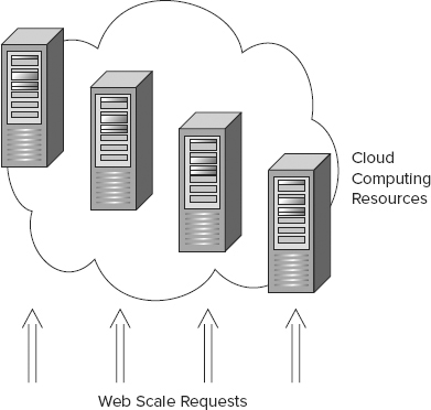
Fulfilling user requests as quickly as possible is the bread and butter of backend services, and maintaining performance during spikes in application usage presents a significant challenge to service developers. By far the most successful way to increase server availability is to run cloud-based applications on large arrays of identical hosts. Application requests usually run entirely independent of each other, and as long as the underlying persistence mechanism supports parallel access, it’s possible to support large numbers of simultaneous requests simply by throwing large numbers of commodity servers at an application. Each user sees that the application performs well for them and does not need to know that perhaps thousands of other machines performed the exact same operation for other users at the same time. Figure 7-1 illustrates the cloud. It’s called the cloud because you don’t know where or how many hosts run your application; they are just available on demand, as from an amorphous “cloud” of resources.

FIGURE 7-1

The Scale of Mobile

As this book describes, supporting native Android clients involves a significant set of challenges for service developers. However, when you consider the domain logic of applications, you’ll find that there are more similarities than differences between mobile and desktop service development. Both clients require REST support and use similar domain objects. The most drastic difference, besides a smaller screen, is the sheer scale of clients that can make a request on a mobile service. In the United States, not everyone in a household has his or her own laptop or desktop, but almost everyone has at least one device. In developing nations, extremely cheap Android tablets are bringing the Internet to billions of people who have never used a computer.

Using Push Messages

Given the sheer volume of traffic possible with mobile computing, it’s critical to consider strategies that reduce redundant client communication. Client-based polling represents a glaring form of unnecessary communication; push-based protocols allow the service to inform clients about relevant changes, rather than clients constantly asking if “they are there yet.” Chapter 6 introduced a lightweight synchronization protocol that can work well with a push-based model, where the push message itself can either directly include synchronization state, or simply indicate that a client should initiate synchronization itself. When you think about hundreds of millions of devices all simultaneously initiating wasteful poll requests, a push-based approach becomes highly desirable.

It’s relatively simple for a given device to initiate contact with a service, but it’s not nearly as straightforward for a service to contact a device. Devices run on intermittently connected networks where it’s not even guaranteed that a service will physically be able to contact a device — if there is even a consistent way of contacting devices. Devices run on WiFi and a wide variety of 3G and 4G carrier networks. Sometimes devices have IP addresses and sometimes they do not. Most of the time applications do not have permission to listen on ports to create a service. Traditionally, the simplest and perhaps the most reliable and cross-platform way of sending a message to a device is to use an SMS message. As primitive as it sounds, SMS works pretty well. Another common means to implement push capabilities is by having a client just leave open a persistent HTTP connection through which a service can push messages to the client for the duration of the connection.

Synchronization

Chapter 6 introduced synchronization from the perspective of backend development, but with no particular emphasis on scaling or implementation. In this section, you’ll consider how the combination of push and synchronization technology can pair to create a drastic reduction in traffic and polling. Picture the following scenario:

• Clients can make changes locally without needing to poll the service, since they can rely on push messages (the server can notify on change) to stay up to date.
• The client does not need to create a new request for every change it makes; a synchronization request can batch client changes.
• The service is free to accept changes from and sync with other devices.
• Clients can lose network connectivity and remain functional, since the client has local state it can edit and display.
• The developer has flexibility in configuring synchronization times — periodically or as needed depending on system resources.

As you can see, a push and synchronization-based system has significant advantages over polling CRUD protocols. Consequently, this book spends a significant amount of time getting you to think about specific sync-based approaches.

Persistence in the Cloud: From SQL to NoSQL

Of the many challenging aspects of designing an app to have a flexible and scalable architecture, persistence represents one of the thorniest problems. Recent trends in data-driven applications have involved the use of traditional SQL as well as newer scalable architectures that rely on a persistence technology called NoSQL. The next sections address important strengths and weaknesses of SQL and discuss why NoSQL was created to maximize scalability for modern applications. Keep in mind that the following discussions are a matter of some debate.

SQL Databases

Many proponents of NoSQL systems argue that the nature of SQL itself tends toward the creation of static schema that have limited capability to evolve as underlying changes in schema become necessary. By contrast, NoSQL approaches can handle such changes intrinsically. Although it’s true that schema changes can be difficult to implement in a typical SQL model, it’s actually straightforward to create a SQL schema that can accommodate changes over time. Consider the schemas shown in Listings 7-1 and 7-2.

LISTING 7-1: Static schema

CREATE TABLE contacts (
    id INT NOT NULL AUTO_INCREMENT PRIMARY KEY,
    firstName VARCHAR(50),
    middleName VARCHAR(50),
    lastName VARCHAR(100)
);

LISTING 7-2: Dynamic schema

CREATE TABLE KeyValue (
    id INT NOT NULL AUTO_INCREMENT PRIMARY KEY,
    objectId INT,
    key VARCHAR(100),
    value VARCHAR(100)
);

Suppose your application inserted thousands of records into the table for Listing 7-1, and you needed to add a new field for a second middle name, due to a few users having non-standard names. SQL supports schema modification using the alter table command. However, changing the table structure would require all contacts to have a second middle name field, which would likely be overkill and would waste resources.

Consider the alternative schema in Listing 7-2. This schema is similar to the KeyValueContentProvider content provider from Chapter 4. With only a minimal amount of extra overhead, you can store objects with arbitrary fields all in the same table. To retrieve a complete object, you just select for a given objectID, and you will get a result set with rows (instead of columns) that are the fields of the object. “Schema changes” in this scenario become simply a matter of adding and deleting KeyValue rows and maintaining an object ID.

You might be thinking, okay, it’s possible to create flexible schema in SQL, but is it convenient? The answer is a matter of opinion, but as you’ll soon learn, newer schema-less or NoSQL systems can handle such behavior with less up-front design. For example, with MongoDB, a popular NoSQL database, all database rows in a table are JavaScript objects; you don’t need to define flexible schema, you just insert objects that have different fields into the same table, and MongoDB, supports their storage by default.

SQL Indexes

SQL has supported indexes out of the box for most of its multi-decade history. When a developer needs to speed up searching on a particular column, it’s as easy as declaring an index on the relevant table and column, as is shown with the line that follows using the table from the previous chapter:

create index updateTimeIndex on contact (updateTime);

This declaration is all an application needs to create and maintain an index as data is inserted and deleted over time. SQL indexes have made it very easy to enable efficient lookup times for a highly significant number of web applications. Although this is a straightforward observation, please keep it in mind for the upcoming discussion on NoSQL databases.

SQL Transactions

SQL supports a wide array of powerful programming functions, the most significant of which is transactional support. Transactions ensure that a set of database operations has atomic or “all or none” behavior, guaranteeing that errors do not leave the database in an inconsistent state if only part of the set operations were to succeed (for example, a bank account transaction whereby a debit succeeds, but an intended subsequent credit fails). SQL databases have rich transaction support that guarantees so-called ACID properties (Atomicity, Consistency, Isolation, and Durability) for all transactions on a database.

Transactions also have a standardized locking level scheme, whereby applications specify the level of concurrency allowed for each transaction. The level of most isolation is SERIALIZABLE or no concurrent access at all. Clearly higher isolation levels reduce parallel scalability, when a single user can have exclusive access to data.

Single Host Database

In previous chapters, you saw how SQL, and SQLite in particular, provides fine-grained query capabilities and high-level features like transaction support and the ability to apply indexes to column data.

When considering scalability requirements for web scale solutions, such expressiveness does not come without cost. To start, the most widely used SQL databases — such as MySQL and PostgreSQL — represent a single point of failure where a single machine stores a database for what might be a cluster of application containers serving parts of a single application in parallel (see Figure 7-2).

FIGURE 7-2

Scaling Relationships

Providing a significant basis for relationships between entries, the SQL join feature is among the most useful of traditional database operations. Unfortunately it’s hard to distribute joins across parallel data hosts, due to the inherent expense of accessing join data that resides on more than one machine. To understand the problem a little better, consider that in a scalable persistence solution, an element of data will reside on roughly a single machine (data redundancy for robustness aside). Assembling data in multiple tables and columns needed for a join is likely to require many round trips to different hosts. The communication and data marshaling make joins expensive. Additionally, you’ll see how hard drive seek time plays a significant role.

Database File Format

The file format that a database uses to persist information to disk has significant implications for the performance of the database. For years, SQL databases have innovated in various ways with their file format (like PostgreSQL and its versioning system), but the high-level layout of data has been the same, as discussed in the following sections.

Row-Oriented

The SQL create table command enables the declaration of two-dimensional data structures. To support this function, traditional SQL databases use a two-dimensional row-oriented format. So a very simple row oriented table could look like Listing 7-3, where a row contains id, firstName, lastName, and age columns.

LISTING 7-3: An example two-dimensional row-oriented table

id, firstName, lastName, age
0, jon, smith, 12
1, kate, hughes, 32
2, joan, molan, 29

As concerns database implementers, seeking to a particular location in a file is as expensive as seeking and loading a moderate amount of data (such as 1MB) from that file. Seeks take a long time due to the need to physically orient a hard drive to the location of relevant data — once in position it’s ideal if the data nearby is useful. For a given SQL query, if you were to search on an indexed firstName, you would incur as many seeks as there are rows with the name selected in the query. A query with no index (the default) would need a seek for every row in the table.

As you can see, traditional SQL database designs have some issues that could limit their use in massively scalable deployments.

Column-Oriented

So take a step back for a minute. Is there a way to structure data to turn hard disk seek limitations to the advantage of the database designer? In contrast to the row-oriented format used in SQL databases, consider a column-oriented approach. The layout shown in Listing 7-4 reformats the row-based data from the earlier section to use columns instead.

LISTING 7-4: An example two-dimensional column-oriented table

id: 0, 1, 2
firstName: jon, kate, joan
lastName: smith, hughes, molan
age: 12, 32, 29

Recall that multiple seek operations take more time than one seek plus reading up to about 1MB of data. Suppose you wanted to compute the average age of all people in the table in Listing 7-4. With one seek, you could read out an entire column and then compute the average in a single pass. In contrast, a row-oriented format would require many seeks and reads to load the rows for all people into memory and then select each age to compute the average. For certain types of operations, called aggregate functions, columnar organization has enabled vast performance improvement.

Due to its heavy use in data intensive applications, it’s worth pointing out that sorting is effectively an aggregate function as well. If it’s quick to read out values of a column into memory, you can subsequently sort those values in memory. So for example, if you have a query that sorts by first name, it’s much faster to have all first names in one file, rather than spread across a set of rows, each of which would need its own seek to read a single first name.

For more information on this topic, see Wikipedia:

http://en.wikipedia.org/wiki/Column-oriented_DBMS

Record Size

Because of the way the SQL language defines schema, a create table is effectively a declaration of the sizes of the data types in a row, and the size of the two-dimensional structure that holds them. The create table statement does not allow for varying element sizes. Of course, dropping the SQL language would mean you could support that capability.

NoSQL Persistence

As discussed, the demands of web and mobile scalability have driven the design of large-scale storage systems. As you might have guessed, distributing request load and avoiding unnecessary seek operations held critical importance in meeting scalability requirements. All of the major so-called “NoSQL” databases — like Amazon DynamoDB, Google App Engine Datastore, Cassandra, and MongoDB — use a column-oriented format for the reasons just discussed, and the presence of an ID or key is the only requirement they place on the number of fields for a given element. In these systems it does not make sense to think of a “column” as similar to a column in a SQL table. This NoSQL key is a lot more like a key/value pair in a persistent map data structure. As their name suggests, none of these databases support the SQL language, and they do not require that records contain the same number of fields or have a static size.

Searching NoSQL

So far, NoSQL databases sound like a pretty solid way of meeting web scale requirements. They minimize hard disk overhead and allow specific column flexibility not found in SQL. But do they have any drawbacks? The answer seems to be a clear yes. For example, searching with Amazon DynamoDB is entirely unlike querying a SQL database and in many ways is much more primitive. You don’t get a nice index keyword, and the database does not automatically update indexes on your behalf. Your application must include code that creates and updates its own index whenever you insert or delete new data. Perhaps not surprisingly, the reason for such “retro” coding techniques is a result of aggressive optimization on the part of the database providers. Using a primitive API enables database developers to increase the performance of their service platform as a whole, as you’ll see in the next section.

NoSQL Scan Queries

Querying a NoSQL database depends significantly on intelligent sorting of column-based data. The Google App Engine Datastore (which is built on a NoSQL technology called BigTable) sorts column data using a hierarchical primary key. The basic layout of BigTable consists of a column containing rows with the following layout:

Row Name: Column Set

It looks somewhat like a traditional database table, but the column is the row name and its column set — only the row name is directly searchable. The row name or key is “known” to the implementation of the database and all data in the database is sorted on it. The result of this simple structure is that database queries simply scan the database for row names or, alternatively, for a range of row names. In the case of BigTable, you can search based on a prefix. You can return all row names that start with a given prefix (such as all the names that begin with the letters “ca”) or return a range of row names starting with one prefix and ending with another. To understand a little better how this works for BigTable, consider Figure 7-3, which shows the parent-child relationships of rows in BigTable.

FIGURE 7-3

What you see in Figure 7-3 illustrates the hierarchical key structure used with BigTable. Keys are sorted according to name in hierarchical order. This clever arrangement allows not only fast scanning lookup, but fast scanning of an element and its descendants. Such organization greatly benefits any data with a hierarchical relationship, such as geodata (for example, cities in a state), players on a team, and so on. The keys in Figure 7-3 are built from a construct known as an entity that this chapter will explore further in the App Engine code example later.

Significant operations like search are extremely fast with NoSQL databases, but the downside of less structure is the significant complexity pushed out of the persistence layer into the application space. Done right, NoSQL applications may scale better and run faster, but developers must address tricky synchronization and performance issues that the database solves with SQL-based approaches.

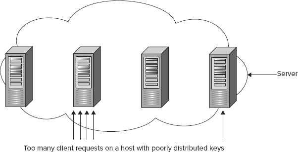
Key Distribution

Column-oriented databases that “shard” their data based on row keys rely on applications to evenly distribute data across different hosts. When applications fail to achieve this distribution, scalability will degrade when the system becomes less than fully distributed — data will reside on fewer hosts than possible thus increasing load on specific servers. Such overload points are known as “hot spots” or “hot keys” and developers can avoid them by using a sufficiently distributed hash key. Figure 7-4 shows key distribution and scalability hot spots.

FIGURE 7-4

DESIGN CONSIDERATIONS FOR SCALABLE PERSISTENCE

Now that you understand the basics of scalable cloud persistence and some pros and cons of using SQL, the next few sections take the discussion into practical design matters like what to consider when selecting a database style and when to update indexes, among others.

To SQL or Not to SQL?

Application developers making a decision about whether to use SQL should consider a number of variables:

• Does your application handle vast amounts of data, on the order of serving millions of users?
• Will the structure of your data benefit from using a flexible column set? Will you need to add or remove columns on the fly?
• Does your application require sophisticated query support?
• Do you have the resources to host your own server farm?
• Can your engineering team handle the added development complexity of NoSQL?

If your application will use only moderate amounts of web traffic (such as what most web applications encounter), the limited querying capabilities of NoSQL could prove to be a significant hurdle, and without much benefit. In many cases, starting with or using SQL will deliver the flexibility you need and will help you to develop safer applications. On the other hand, large datasets work well with NoSQL due to its fast scanning capabilities.

Using Schema

Even with NoSQL datastores, developers will find it useful to employ a schema-like definition for their application data model. Although NoSQL does not require similar columns between elements, it’s useful if elements at least share a subset of fields. For example, a business contact could support all the same fields as a contact, but also add a business phone number and business e-mail. Often the form of such schema will bind to objects in the developer language of choice (such as a class in Python or Java). You’ll see how this works later in the chapter in the Google code example with queries on the contact class.

Handling NoSQL Indexes

SQL or NoSQL, data indexes — or precomputed answers to queries — are the primary method of improving the performance of persistence queries. As mentioned, implementing your own indexes with NoSQL databases adds significant complexity to your application. It’s possible to avoid some of this complexity by integrating an existing search solution, such as Apache Lucene or Solr, into your product. So, instead of building your own indexes, you can integrate a search engine into your application and use it to implement queries.

Updating Indexes Asynchronously

Indexes must reflect the current state of the database in order to return accurate results, which means indexes must be updated when data changes. The work of managing the database while satisfying user requests has the potential to degrade request performance. A common method of dealing with this overhead is to handle it asynchronously from the requests themselves. It’s convenient to use a persistent task queue. Amazon released a tool called Amazon SQS, which is covered shortly.

Stateless Design

Continuing to hit on the main theme of the chapter, a successful cloud data model will seek to maximize scalability of requests. A stateless service stores all persistence information in its data tier and does not seek to reuse state across requests. A stateless request relies only on the content of the request and persistent state in the database.

A typical example of shared state is a session-oriented protocol where session information must be part of every request. Shared state requires blocking while different hosts access the shared information where it happens to live in the database, and is generally the enemy of parallel execution.

Eventual Consistency

NoSQL systems generally do not strive to maintain ACID-level consistency due to the noted trade-off between exclusive access to data and optimal scalability. Indeed the formal CAP theorem remarks on the extreme difficulty of building a system that is strongly consistent, highly available, and fault tolerant:

http://en.wikipedia.org/wiki/CAP_theorem

Most NoSQL systems, like DynamoDB, do not support complex transactions. Google Datastore is a notable exception and does support them. On systems that do not support transactions, how do NoSQL applications guarantee consistent state? Most modern cloud services rely on the principle of eventual consistency. This principle states that if the users were to all of a sudden stop making requests on a given service, the data for the service would be brought to a consistent state. The database would have time to edit its internal state to make the effects of each request consistent.

Optimistic Concurrency Control

Massive simultaneous request execution provides the mechanism by which web scale applications achieve high levels of scalability. With so many clients hitting the data simultaneously on different machines, and only eventual consistency to hold the system together, it might seem that preventing an inconsistent state would be impossible.

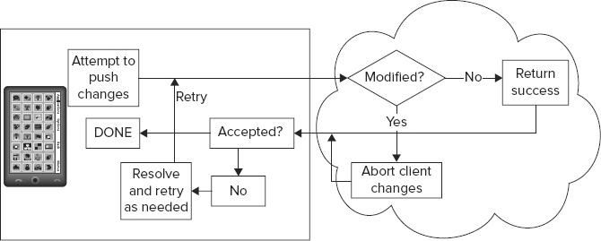
As it turns out, an extremely simple rule called optimistic concurrency control provides a solution. Imagine that when a client attempted to submit changes to the database, the database detected whether any changes from the client were in conflict with changes already in the service. Detecting changes in the service is application-specific but can be as simple as checking modification times or version numbers on data. If the service does find a conflict, the client aborts its change and gets the latest state from the service. When the client is ready to resubmit, the process repeats, until the service accepts the client’s changes, and the client’s data gets written to the service datastore (see Figure 7-5). The rule is called “optimistic” because the client always makes its best attempt to commit data. Typical usage patterns suggest that in the majority of cases, it will succeed.

FIGURE 7-5

Load Balancing

To take advantage of simultaneous data requests, an application needs to direct requests across a large number of hosts. Developers call this distribution process load balancing. Most cloud providers support load-balancing functions to make it easier to scale service traffic. For example, Google App Engine provides a built-in load balancer that automatically distributes the requests among your servers, whereas AWS provides a technology called elastic-load-balancing. Making your server stateless is critical to effective load balancing.

Optimizing Costs

One of the most important advantages of using a cloud service is the flexibility to scale up and down as needed, which means you can add more servers during peak times and reduce service use during down times. Your application only uses resources when it needs them. If you own your own bank of servers capable of handling a massive peak, those servers are likely to sit idle and cost you money during slow periods of traffic.

LOOKING AT POPULAR CLOUD PROVIDERS

Cloud-based hosting has grown to encompass a vast technology industry. Most major technology corporations host cloud platforms, but a few clear winners have emerged. The next section highlights a few of them.

Amazon AWS

Amazon hosts a wide array of cloud products to support web applications and backend services, and generally could be regarded as a 900-pound gorilla in cloud hosting services. Amazon provides a large family of complementary technologies, and the following are relevant to the chapter examples:

• DynamoDB — Foremost among these services is DynamoDB, with which you are now well familiar. It’s a scalable column-oriented database for storing structured data.
• Amazon S3 — Amazon Simple Storage Service, designed for storing large data blobs ranging from up to 5 terabytes of data. The service could be used to store any large file, including videos or sensor data, but generally does not hold structured data.
• Amazon SQS — A distributed queue-based messaging service that supports guarantees on message delivery. Amazon SQS supports “at most once” message delivery semantics, meaning an app can resend a message without fear of redundant application. Many readers will be familiar with the Java Message Service (JMS); the SQS fulfills the same role. Amazon SQS might be used to deliver periodic Android sensor data to a scientific monitoring service.

  ---

  NOTE The chapter’s example code suggests a use for SQS in conjunction with transaction support for DynamoDB. The AWS code walkthrough discusses how it would work.

  ---

• AWS Management Console — In addition to supporting cutting edge cloud services, Amazon also supports easy-to-use online management tools for creating, modifying, and monitoring running services.
• AWS Free Usage Tier — Most Amazon services have some sort of free introductory usage. As of the time of writing of this book, DynamoDB supports 100MB of storage, five units of write capacity (5 writes/second), and 10 units of read capacity (10 reads/second), available to new and existing customers. With Amazon, each service has its own free plan:

Google App Engine

Clearly Google itself is a highly significant player in the cloud hosting space. Like Amazon, Google also supports a large suite of mature, complementary services for running third-party applications on Google’s formidable cloud infrastructure. Here are a few to get started:

• Datastore — This is Google’s persistence service based on the structured data, column-organized BigTable, as discussed in this chapter.
• Blob store — Large object data storage, for objects that will not fit in Google’s structured datastore. Blob files are submitted using HTTP operations, often with a simple form.
• Memcache API — A high-performance distributed in-memory cache that applications access in front of persistent storage, like Datastore. Memcache uses the JCache API, a standard caching interface. Redundant queries accessing the same data should make use of the memcache API. The memcache API is designed to work in a highly scalable load-balanced environment.

For App Engine pricing:

https://cloud.google.com/pricing/

Joyent: Hosted MongoDB+node.js

The Joyent cloud-hosting platform optimizes the performance of several widely popular cloud-computing technologies not presented in this version of Enterprise Android. Joyent is notable as having hosted Twitter for a time — certainly a web scale application. These components include:

• MongoDB — A horizontally scaled, completely JSON-oriented columnar style database. MongoDB is a “document-centric” database in which developers can directly insert or delete JSON objects with no requirement to pre-define schema for storage.
• node.js — An event-driven service development platform that leverages client-side web development mindshare by using JavaScript as a server-side development technology. Developers write services completely in JavaScript. Node.js strongly defines methods of interaction, so all services running on a node.js installation integrate with each other by default.
• Hadoop — A platform that supports data-intensive applications, supporting petabytes of data. Hadoop supports a computational paradigm known as MapReduce that enables processing of large datasets. MapReduce breaks up large computing problems into small pieces so that they can be processed on parallel hardware:

http://en.wikipedia.org/wiki/Hadoop

Red Hat OpenShift

Red Hat has created an open source cloud-computing platform called OpenShift. OpenShift is notable because it takes a different approach than some of the other providers. Where Amazon or Google create an explicit API for their services that they intend developers to consume directly, OpenShift allows developers to select a pre-configured, usually open source API for development. Developers also have the option to define their own new “cartridge” or set of OpenShift APIs. The result is that developers end up using the API of their choice while still getting the benefit of cloud hosting. For those concerned about “vendor lock-in,” becoming too directly dependent on the APIs of any particular vendor, OpenShift can potentially help developers avoid this pitfall.

OpenShift supports the following set of default cartridges, which provide support for environments from JBoss (a popular Java server technology) to Ruby (a popular open source programming language):

https://openshift.redhat.com/community/developers/technologies

Now with enough background on cloud computing and service development technologies, you’re ready to jump into the chapter code examples.

EXPLORING THE CODE EXAMPLES

This chapter provides contact service implementations for the two most popular cloud service platforms discussed in this chapter: Amazon Web Services (AWS) and Google App Engine. The examples build on the work done in Chapter 6 with the Spring-based contacts services — you’ll build two new contact service variants for both of these service platforms. The examples will walk through specific code that demonstrates topics this chapter has covered so far, such as building NoSQL indexes and using range queries. Each service reuses much of the code from Chapter 6, taking advantage of its three-tier architecture. With some configuration aside, these services only need to provide their own new implementation of the contact DAO interface. In a production deployment this architecture would mean that you could easily switch between cloud providers and databases. This is a nice advantage given competing prices and designs prevalent in today’s cloud services market.

Note that the idea behind these examples is to give you a taste of what it’s like to develop in each environment and to get you thinking about how to solve common mobile data problems with these technologies. The examples are not intended to provide a comprehensive introduction to the relevant platforms. Authors have filled volumes on both of them.

The Contacts DAO Interface (Again)

Recall the contacts DAO interface introduced in the previous chapter. The DAO interface for this chapter includes methods for finding and manipulating contacts, as shown in Listing 7-5.

LISTING 7-5: Contact DAO review

  package com.wiley.demo.android.dao;
 
  import java.io.IOException;
  import java.util.List;
 
  import com.wiley.demo.android.dataModel.Contact;
 
  public interface ContactDao {
      Contact getContact(String userId, String id) throws IOException;
     String storeOrUpdateContact(String userId, Contact contact) throws IOException;
     List<Contact> findContactFirstName(String userId, String firstName, 
         int start, int numOfmatches);
     List<Contact> findChanged(String userId, long timestamp, int start, int 
           numOfmatches);
     void delete(String userId, String id) throws IOException;
     List<Contact> getAll(String userId, int start, int numOfmatches) throws 
           IOException;
 }

The remaining sections of the chapter will cover example code for implementations of this interface using Amazon DynamoDB and Google App Engine.

Writing the Code: Amazon Contacts Service

This example focuses on how to integrate with Amazon Web Services and how the tiers of the contact service have changed to make use of DynamoDB, thus enabling the contacts service on the highly available Amazon cloud. This section of the chapter investigates the contact DAO implementation as implemented on Amazon’s DynamoDB. You can find a complete working example in the following directory:

$CODE/awsServiceContacts

Prepare: Prerequisites and Getting Started

Chapter 6 covered all the requirements for developing a Java web application based on Spring, Jackson, and the application container, Tomcat. The Amazon Web Services DynamoDB service example leverages many of these same tools, but also requires the presence of the Amazon Web Services SDK, an AWS account, and credentials.

Step 1: Create an Amazon Account

Create an Amazon AWS account if you do not have one. To create the account, go to http://aws.amazon.com/ and click the Sign Up button. You should be able to follow the instructions from that point to create the account. You will need a credit card to complete sign-up.

Step 2: Configure DynamoDB with Application Schema

Once you have created an account, you can visit the AWS management console at:

https://console.aws.amazon.com

From there, click the DynamoDB link under the Database category. This takes you to the UI for managing the DynamoDB. Follow the instructions there to create application tables in DynamoDB — the table wizard may pop up by default.

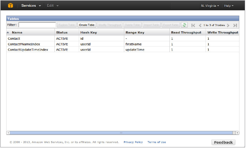
Working with AWS is different than working with traditional SQL databases — schema management takes place in an online editing tool, rather than with a source code-based SQL language. At the top of the page in the Dynamo DB section, you should see a row of buttons. Find the one labeled Create Table and repeat the table creation process for the next tables. You need to create the following three tables: Contact,ContactFNameIndex, and ContactUpdateTimeIndex.

• The Contact table stores contact data. When creating each table, you will need to decide whether the table will use a hash key and range key, or a hash key only. This table needs only a hash key, which the UI will prompt you to add as a hash attribute name. Click the appropriate radio button. The name should be id.

• ContactFNameIndex stores the index for searching on the first name. This table needs both a hash key and a range key, and you should define the type of the keys as String. The hash attribute name is userId, and the range attribute name is firstName.

• ContactUpdateTimeIndex stores the index for searching on update time. This table needs both hash and range keys, and the range and hash attribute names are userId and updateTime, respectively. Again, the types of the keys are String.

Figure 7-6 shows the Amazon AWS online schema-editing tool showing the schema you’ll need to create to use the contacts service.

FIGURE 7-6

Amazon has provided DynamoDB documentation on its developer site as well:

http://aws.amazon.com/dynamodb/

Step 3: Specify the Read/Write Throughputs

For each table you define, you need to specify the Read Throughput and the Write Throughput. If you are using the AWS free tier account, set both Read Throughput and Write Throughput capacity units to 2 to avoid being charged. The higher you go, the more you will pay. You can find specific AWS pricing details on their site:

http://aws.amazon.com/dynamodb/pricing/

Click Continue. The next screen optionally allows you to monitor your request rates and set throughput alarms. We won’t be doing that for our example, so just enter an e-mail address for notification and click Continue to finish table creation.

The final page provides a summary for your review. Click Create, and you’ll be taken to the Services page, providing both editing capabilities and detailed information about the table(s) you just created.

Step 4: Create Access Credentials

Before your client can communicate with AWS, you need to create an access key, as follows: AWS Management Console Your Name menu My Account Security Credentials (on the left).

This brings you to the AWS security credentials page where you can create an access key with: (Preferred) https://console.aws.amazon.com/iam/home?#security_credential Access Keys Create New Root Key

Create the key and download its corresponding csv file—it contains the access and secret keys.

Or use: (Deprecated) Access Credentials create new access key

Your key will be displayed; use the UI to show the secret key.

Step 5: Install Amazon Web Services SDK (Optional)

To work with Amazon Web Services, you’ll need to download the SDK from Amazon’s development center from the following location:

http://aws.amazon.com/sdkforjava/

Step 6: Add Security Credentials

Add the access key and secret access key to the file:

$CODE/awsServiceContacts/src/main/resources/com/enterpriseandroid/awsContacts
/dao/impl/AwsCredentials.properties

By entering the keys as follows:

1 secretKey=<Insert your secret key here>
2 accessKey=<Insert your access key here> 

Finally, change the following field:

$CODE/awsServiceContacts/src/main/java/com/enterpriseandroid/awsContacts
/rest/ContactController.USER_ID

to be your Amazon account user name.

Step 7: Tools and Software Stack

This chapter has fewer libraries to cover in its software stack than in the previous chapter, given how much code is the same for the presentation and logic tiers. The Amazon SDK is the only new tool in the software stack, and its APIs are only used in the Data tier DAO. All the other software dependencies from Chapter 6 apply here as well. For your convenience, the project ivy.xml contains a dependency on the App Engine SDK, as follows:

<dependency org="com.amazonaws" name="aws-java-sdk" rev="1.3.26" />

Example Code: Replacement Contact DAO

As mentioned, the Amazon sample code demonstrates how to port the RESTful contacts service to the Amazon cloud. The class, ContactDaoDynamoDBImpl, provides the relevant implementation code for the contact’s DAO, which contains significant differences from the SQL or Hibernate versions of the previous chapter.

Instead, the Dynamo API client class, AmazonDynamoDBClient, supports all persistence operations, which in turn uses the Amazon API for persistence as follows:

• The example uses a less sophisticated version of object serialization for persistence due to the way that Dynamo structures return values. The Dynamo client returns objects in the form of Java maps. Consequently, the example accesses object field values using simple constant access, as follows:

  item.get(FIRST_NAME).getS();

• As discussed earlier in the chapter, DynamoDB uses scan queries. To find contacts, the DAO implementation uses the composite string key userId:contactID.
• The code uses two contact fields to find contacts to support the contacts sync algorithm: contact first name and contact update time.
• As mentioned earlier, DynamoDB does not support SQL style indexes. As a result, the code also contains two methods for updating indexes for its two search fields.

Listing 7-6 shows the documentation for the AWS DAO class.

LISTING 7-6: DAO implementation for DynamoDB

 package com.wiley.demo.android.dao.impl;
 
 import com.amazonaws.ClientConfiguration;
 import com.amazonaws.auth.AWSCredentials;
 import com.amazonaws.auth.PropertiesCredentials;
 import com.amazonaws.services.dynamodb.AmazonDynamoDBClient;
 import com.amazonaws.services.dynamodb.model.*;
 import com.wiley.demo.android.dao.ContactDao;
 import com.wiley.demo.android.dataModel.Contact;
 
 import java.io.IOException;
 import java.util.ArrayList;
 import java.util.HashMap;
 import java.util.List;
 import java.util.Map;
 import java.util.UUID;
 
 /**
  * Enterprise Android contacts RESTful service implementation that uses the
  * Amazon Dynamo DB API for scalable, hosted persistence.
  */
 public class ContactDaoDynamoDBImpl implements ContactDao {
     private final String ID = "id";

Key names for the contacts search fields, first name, and last name are as follows:

     private final String FIRST_NAME = "firstName";
     private final String LAST_NAME = "lastName";
     private final String EMAIL = "email";
     private final String UPDATE_TIME = "updateTime";
     private final String VERSION = "version";
     private final String HASH_KEY = "userId";

These are the names of the search field indexes. The relevant indexes get updated in the methods updateUpdateTimeIndex and updateFnameIndex.

     private final String FIRST_NAME_INDEX_TABLE = "ContactFNameIndex";
     private final String UPDATE_TIME_INDEX = "ContactUpdateTimeIndex";
     private final String CONTACT_TABLE = "Contact";
 
     private AmazonDynamoDBClient client;
 
     public ContactDaoDynamoDBImpl() throws IOException {

This code initializes the Amazon DynamoDB client with credentials obtained from the properties file, AwsCredentials.properties.

         AWSCredentials credentials = new PropertiesCredentials(
                 ContactDaoDynamoDBImpl.class
                         .getResourceAsStream("AwsCredentials.properties"));
 
         ClientConfiguration config = new ClientConfiguration();
         client =  new AmazonDynamoDBClient(credentials, config);
     }
 
     @Override

The method for getting a contact takes a userId and a contact id. It uses the Amazon request class, GetItemRequest, to build a request consisting of a table name and a composite key, which has the aforementioned format: userId:contactId. DynamoDB will service the request with a fast scanning search.

     public Contact getContact(String userId, String id) throws IOException {
 
 //        List<String> attributesToGet = new ArrayList<String>(
 //                Arrays.asList(ID, FIRST_NAME, LAST_NAME, EMAIL,
 //                        UPDATE_TIME, VERSION));
 
         // Get a contact with the composed string key, userId:id to identify
         // the row for the contact. We're not explicitly specifying the
         // columns to get, since we want all of the columns. But you could
         // specify columns using the code commented out above and below.
         GetItemRequest getItemRequest = new GetItemRequest()
                 .withTableName(CONTACT_TABLE)
                 .withKey(new Key().withHashKeyElement(new AttributeValue()
                         .withS(this.composeKeys(userId, id))))
 //                .withAttributesToGet(attributesToGet)
                 .withConsistentRead(true);
 
         awsQuotaDelay();
 

The DAO implementation delegates to the Dynamo client to get the results of the request.

         GetItemResult result = client.getItem(getItemRequest);
         Map<String, AttributeValue> item = result.getItem();
         if (item == null) {
             return null;
         }

When the results return as maps, a utility method converts them into contact objects.

         return item2Contact(item);
     }
 

The method storeOrUpdateContact adds a contact under the given userId. The contact gets updated if it already exists.

     @Override
     public String storeOrUpdateContact(String userId, Contact contact)
             throws IOException
     {
         Map<String, ExpectedAttributeValue> expectedValues =
                 new HashMap<String, ExpectedAttributeValue>();
         Contact oldContact;
 
         String oldFirstName = null;
         long oldUpdateTime = -1;
 
         if (contact.getVersion() != 0) {
             expectedValues.put(VERSION,
                     new ExpectedAttributeValue()
                             .withValue(new AttributeValue()
                                     .withN(Long
                                             .toString(contact.getVersion()))));
             oldContact = getContact(userId, contact.getId());
             if ( oldContact != null) {
                 oldUpdateTime = oldContact.getUpdateTime();
                 oldFirstName = oldContact.getFirstName();
             }
         }
 
         contact.setUpdateTime(System.currentTimeMillis());
 

Create the values for the contact object, making sure to increment the version, and set the update time to the current time. The scan key is the same as before, userId:contactID.

         Map<String, AttributeValue> item = contactToItem(contact);
         item.put(VERSION, new AttributeValue()
                 .withN(Long.toString(contact.getVersion() + 1)));
         item.put(ID, new AttributeValue().
                 withS(composeKeys(userId, contact.getId())));
 
         /***
          * AWS does not provide transaction support, and cannot guarantee that
          * all the writes to DynamoDB are successful. To avoid this problem, we
          * recommend using AWS SQS service. The idea is to wrap both update
          * operations into a task, and then put the task into SQS. If and only
          * if both operations succeed, would we remove the task from the SQS.
          */
         putItem(CONTACT_TABLE, item, expectedValues);

Insert the given contacts object into the contact table, making sure to update the update time index and the first name index. Take note that this is where the code needs to manually update its own index. With SQL you would not need to remember to add this type of code — it’s critical to performance that you maintain indexes correctly.

         updateUpdateTimeIndex(userId, oldUpdateTime, contact);
         updateFnameIndex(userId, contact.g etFirstName(),
                 oldFirstName, contact.getId());
 
         return contact.getId();
     }
 
     private void updateUpdateTimeIndex(String userId,
                                        long oldUpdatTime, Contact contact)
     {
         if (oldUpdatTime == contact.getUpdateTime() ) {
             return;
         }
 

Updating the update time index consists of putting an item into the update time index table, with the hash key of userId and a composite update time key of updateTime:contactID.

The newly inserted object enables lookup by userId of the lastUpdate time of a contact with the given contactID.

         Map<String, AttributeValue> item =
                 new HashMap<String, AttributeValue>();
         item.put(HASH_KEY, new AttributeValue().withS(userId));
         item.put(UPDATE_TIME, new AttributeValue().
                 withS(composeKeys(Long.toString(contact.getUpdateTime()),
                         contact.getId())));
         putItem(UPDATE_TIME_INDEX, item, null);
         if ( oldUpdatTime > 0  ) {
             // delete the old index
             deleteDo(userId,
                     composeKeys(Long.toString(oldUpdatTime), contact.getId()),
                     UPDATE_TIME_INDEX);
         }
     }
 
     private void updateFnameIndex(String hashKey,
                                   String fname, String oldFirstName, String id)
     {
         if (oldFirstName !=null && oldFirstName.equals(fname)) {
             return;
         }
 
         Map<String, AttributeValue> item =
                 new HashMap<String, AttributeValue>();
         item.put(HASH_KEY, new AttributeValue().withS(hashKey));
         item.put(FIRST_NAME, new AttributeValue()
                 .withS(composeKeys(fname, id)));
         putItem(FIRST_NAME_INDEX_TABLE, item, null);

Here, the code updates the first name index. Recall that the hash key in this case is the contact first name. So in this case, the HASH_KEY = userId, and a first name attribute consists of a composed key, firstName:contactID. This code sets the two fields that are the hash key and the range key used to locate contact data in the example DynamoDB.

Not pretty compared to a SQL index, but still an index of sorts — and you don’t have to host your own machines. And at least in this simplified example, it was not too difficult to set up the data model and indexes for contacts.

         if( oldFirstName != null) {
             deleteDo(hashKey, composeKeys(oldFirstName, id),
                     FIRST_NAME_INDEX_TABLE);
         }
     }
 

Here’s a simple utility method for putting items into a Dynamo table:

     private void putItem(String indexName, Map<String, AttributeValue> item,
                          Map<String, ExpectedAttributeValue> expectedValues)
     {
         PutItemRequest putItemRequest = new PutItemRequest()
                 .withTableName(indexName)
                 .withItem(item);
 
         if(expectedValues != null) {
             putItemRequest.withExpected(expectedValues);
         }
 

This call prevents clients from accessing the service too quickly and incurring usage charges.

         awsQuotaDelay();
         client.putItem(putItemRequest);
     }
 
 

This is a search method to find a contact by the first name. The method finds contacts based on a Dynamo condition that matches a scan when a hash key starts with the first name of a given contact. With the query condition established, the method then delegates to the utility query method.

     @Override
     public List<Contact> findContactFirstName(String userId, String firstName,
                                               int start, int numOfmatches)
     {
 
         Condition rangeKeyCondition = new Condition().withComparisonOperator(
                 ComparisonOperator.BEGINS_WITH.toString())
                 .withAttributeValueList(
                 new AttributeValue().withS(firstName));
 
         return query(userId, rangeKeyCondition, start, numOfmatches,
                 FIRST_NAME, FIRST_NAME_INDEX_TABLE);
     }
 
     @Override

The findChanged method also sets up a range key condition to use with a scan query, and then delegates the find request to the query utility.

     public List<Contact> findChanged(String userId, long timestamp, int start,
                                      int numOfmatches)
     {
         Condition rangeKeyCondition = new Condition().withComparisonOperator(
                 ComparisonOperator.GE.toString()).withAttributeValueList(
                 new AttributeValue().withS(Long.toString(timestamp)));
 
         return query(userId, rangeKeyCondition, start, numOfmatches,
                 UPDATE_TIME, this.UPDATE_TIME_INDEX);
     }
 

The query utility method supports Dynamo queries for all RESTful contact operations. The method begins and sets up its main query. It sets the relevant table, hash, and range keys, as well the number of desired matches.

The loop converts maps into contact objects to hold the content results.

     private List<Contact> query(String userId, Condition rangeKeyCondition,
                                 int start,
                                 int numOfmatches, String rangeKeyName,
                                 String table)
     {
         Key lastKeyEvaluated = null;
         List<Contact> ret = new ArrayList<Contact>();
 
         QueryRequest queryRequest = new QueryRequest()
                 .withTableName(table)
                 .withHashKeyValue(new AttributeValue().withS(userId))
                 .withRangeKeyCondition(rangeKeyCondition)
                 .withLimit(numOfmatches)
                 .withExclusiveStartKey(lastKeyEvaluated)
                 .withScanIndexForward(true);
 
         QueryResult result = client.query(queryRequest);
 
         int pos = 0;
         for (Map<String, AttributeValue> indexItem : result.getItems()) {
             pos++;
             if (pos > start ) {
                 String[] ids = fromComposedKeys(indexItem
                         .get(rangeKeyName).getS());
                 Contact contact;
                 try {
                     contact = getContact(userId, ids[1]);
                     if (contact != null) {
                         ret.add(contact);
                     } else {
                         // delete the index if the data does not exists
                         deleteDo(userId, composeKeys(ids[0], ids[1]), table);
                     }
 
                     // awsQuotaDelay();
                 } catch (Exception e) {
                     // if we cannot load the contact, we just continue
                 }
                 if (ret.size() == numOfmatches) {
                     break;
                 }
             }
         }
 
         return ret;
     }
 
     @Override

Since this DAO class needs to maintain its own indexes, the delete method must delete the contact object as well as its associated indexes. Deletion happens by calling the deleteDo query method:

     public void delete(String userId, String id) throws IOException {
         Contact contact = getContact(userId, id);
         deleteDo(composeKeys(userId, id), null, CONTACT_TABLE);
         deleteDo(userId, composeKeys(contact.getFirstName(), id),
                 FIRST_NAME_INDEX_TABLE);
         deleteDo(userId, composeKeys(
                 Long.toString(contact.getUpdateTime()), id),
                 UPDATE_TIME_INDEX);
     }
 

The deleteDo method deletes a data object with the given hashKey and optional rangeKey. The data object is deleted using the DynamoDB client.

     private void deleteDo(String hashKey, String rangeKey, String table) {
         Key key = new Key()
                 .withHashKeyElement(new AttributeValue().withS(hashKey));
 
         if ( rangeKey != null) {
             key = key.withRangeKeyElement(new AttributeValue().withS(rangeKey));
         }
 
         DeleteItemRequest deleteItemRequest = new DeleteItemRequest()
                 .withTableName(table)
                 .withKey(key);
         DeleteItemResult result = client.deleteItem(deleteItemRequest);
     }
 
     @Override
     public List<Contact> getAll(String userId, int start, int numOfmatches)
             throws IOException
     {
         return findChanged(userId, 0, start, numOfmatches );
     }
 

Next is a utility method that converts a map-based Amazon return value into an internally used contact object. Constant values access enables you to set contact fields.

     private Contact item2Contact(Map<String, AttributeValue>item ) {
         Contact contact = new Contact();
         String ids[] = fromComposedKeys(item.get(ID).getS());
         contact.setId(ids[1]);
         contact.setFirstName(item.get(FIRST_NAME).getS());
         contact.setLastName(item.get(LAST_NAME).getS());
         contact.setEmail(item.get(EMAIL).getS());
         contact.setUpdateTime(getLong(item.get(UPDATE_TIME)));
         contact.setVersion(getLong(item.get(VERSION)));
         return contact;
     }
 

Here is the reverse: A utility method that converts a contact into a map-based Amazon item that can be sent to the Amazon API. Constant value access enables you to set map fields from the contact object.

     private Map<String, AttributeValue> contactToItem(Contact contact) {
         String id = contact.getId();
         Map<String, AttributeValue> item =
                 new HashMap<String, AttributeValue>();
         if ( id == null) {
             id = UUID.randomUUID().toString();
             contact.setId(id);
         }
         item.put(ID, new AttributeValue().withS(id));
         item.put(FIRST_NAME, new AttributeValue()
                 .withS(contact.getFirstName()));
         item.put(LAST_NAME, new AttributeValue().withS(contact.getLastName()));
         item.put(EMAIL, new AttributeValue().withS(contact.getEmail()));
         item.put(UPDATE_TIME, new AttributeValue()
                 .withN(Long.toString(contact.getUpdateTime())));
         item.put(VERSION, new AttributeValue()
                 .withN(contact.getVersion().toString()));
         return item;
 
     }
     private Long getLong(AttributeValue attr) {
         return Long.parseLong(attr.getN());
     }
 

The following two methods enable you to split and compose a composite key. A composite key contains a hash key and a range key, and you can use it as an argument in a scan query.

     private String composeKeys(String k1, String k2) {
         return k1 + ":" + k2;
     }
 
     private String[] fromComposedKeys(String k) {
         return k.split(":");
     }
 
     /**
      * The free AWS account only allows 5 read/write per second, so insert a
      * delay to stay under that quota.
      */
     private void awsQuotaDelay() {
         try {
             Thread.sleep(250);
         } catch (InterruptedException e) {
             e.printStackTrace();
         }
     }
 }

Deploy the Service

$CODE/awsServiceContacts/com/enterpriseandroid/awsContacts/dao/impl/ContactDaoDynamoDBV2Impl.java

Now that you’ve developed a Dynamo-based contact service, you’ll need to deploy the code to a Tomcat instance. Since the AWS SDK knows how to talk to the Dynamo backend, you can use a local Tomcat instance, like the one from the last chapter, and as assumed in the instructions that follow, or you can set one up in an Amazon VM. To do this, select My Account AWS Management Console EC2 Launch Instance.

The instructions here describe how to build and deploy the code using Ant or using Eclipse.

Deploying the Code with Ant

cd $CODE/awsServiceContacts 
ant dist

cp dist/awsServiceContacts.war $CATALINA_HOME/webapps

Deploying the Code with Eclipse:

1. Run ant to initialize Eclipse

As with other chapters, you’ll need to use ant to initialize Eclipse:

   cd $CODE/awsServiceContacts
   ant eclipse

2. Import the AWS project directory in Eclipse, as was done in Chapter 6 for springServiceContacts:

   $CODE/awsServiceContacts

Use File Import General Existing Projects into workspace

3. Add a run configuration

Right-click awsServiceContacts in the Package Explorer.

Select Run As Run on server and select the previously added Tomcat Configuration.

Wait for ivy to resolve dependencies.

The AWS service should now be running with persistence in DynamoDB, assuming that the Amazon SDK can connect to AWS services.

Congratulations, you’ve now ported the contacts example to AWS using DynamoDB. You can use both of the Chapter 5 clients with this service simply by changing the client endpoint URL to point to your AWS instance. As in Chapter 6, edit the variable SERVICE in either of the ContactsApplication.java classes in the restfulCachingProviderContacts or syncAdapterContacts projects, or set the system preference RESTfulContact.URI. You now have a working mobile app that can harness the power of the Amazon cloud. Since it’s a good idea to avoid vendor lock-in, next you’ll see how to build an example for another large cloud provider, Google.

Run the Chapter 5 clients and curl against the following local endpoint:

http://localhost:8080/awsServiceContacts/Contacts

Test Your New DynamoDB Service

Test your service using the following commands.

Create contacts:

curl -H "Content-Type: application/json" -X POST -d '{"firstName":"John", 
"lastName":"Smith", "phone":2345678901, "email":"[email protected]" }' 
http://localhost:8080/awsServiceContacts/Contacts

Get contacts:

curl -X GET 
http://localhost:8080/awsServiceContacts/Contacts

Writing the Code: Google App Engine Contacts

The next code walkthrough focuses on how to integrate with Google App Engine and its BigTable-based Datastore. The Google example shares the three-tier architecture with the two previous contacts examples, and the relevant DAO class, the focus of the code walkthrough, is ContactDaoGoogleAppEngineImpl.

Prepare: Prerequisites and Getting Started

The App Engine example also relies on Spring and Tomcat, and of course, requires a Google account for App Engine use, so create one if needed. Log in to your Google account and then go to:

https://appengine.google.com/

Step 1: Create a Google App Engine Service

Click the Create Application button, and then follow the subsequent instructions to create a Google App Engine application. Start by creating a Google “application identifier,” which is a unique string you pick between 6 and 30 lowercase characters; be forewarned, many strings are already taken, we used wileyenterpriseandroidae. Pick a title, select an access level, and sign the terms of use. Your application should now be registered. Save the values that you enter. You’ll use them in subsequent steps.

Step 2: Install the App Engine SDK

To work with App Engine, you’ll need to download the SDK for Java from Google’s developer site at the following location:

https://developers.google.com/appengine/downloads#Google_App_Engine_SDK_for_Java

Of course, Google has significant documentation online:

https://developers.google.com/appengine/

Step 3: Import the Project into Eclipse

Just like you have done for the other service projects in the book so far, import the project into Eclipse:

cd $CODE/googleAppEngineContacts/
ant eclipse

Then import the project folder into Eclipse.

Step 4: Install the Google Plugin for Eclipse

Follow the instructions below to install the Google plugin for Eclipse:

https://developers.google.com/appengine/docs/java/tools/eclipse

Edit the build properties file:

   $CODE/googleAppEngineContacts/build.properties

to enter the path where you installed the App Engine SDK.

Step 5: Configure an Application Identifier

You need to put the application identifier you created in Step 1 into the $CODE/war/WEB-INF/appengine-web.xml, as follows:

 <?xml version="1.0" encoding="utf-8"?>
 <appengine-web-app xmlns="http://appengine.google.com/ns/1.0">
   <application>Add_your_application_id_here</application>
 <version>1</version

Step 6: Create an Application-Specific Password

You won’t be able to deploy updates to your app engine service using your normal account password; instead you must create an application-specific password from the following location:

https://accounts.google.com/IssuedAuthSubTokens?hide_authsub=1#acccess_codes

Application-specific passwords require you to have two-step verification in place, so if you don’t have it on your Google account, you’ll have to turn it on and authorize your computer before completing the process. Be sure to have a phone or a device on which you can receive text messages available. The included link provides a YouTube tutorial on this process.

When invoking update requests from ant or in eclipse, use the following credentials:

• E-mail address—Your account e-mail address
• Password—An application-specific password

Example Code: Replacement Contact DAO

The Google App Engine Datastore sample code illustrates how to port the RESTful contacts service into the Google’s BigTable for structured data. When you examine the App Engine code, it’ll be clear that the App Engine API is in many ways significantly more user friendly than DynamoDB. Google’s Query Language (GQL), loosely based on SQL, has many convenience features that help developers write App Engine services. Such services are not necessarily always beneficial, given that they may interfere with developers’ abilities to optimize performance and scalability in their applications.

The class, ContactDaoAppEngineImpl, provides the relevant implementation code for the contacts DAO. The App Engine contact DAO uses the Datastore Entity API, which revolves around the entity construct, and also Google’s Query Language, which enables SQL-like operations on entities.

Entities Table

The Datastore API stores persistent objects in the form of entities. All entities have a write-once key that uniquely identifies them in the entities table, and a collection of typed properties that contain the data associated with the entity. The entity key contains the following pieces of information:

• Application ID — Uniquely identifies the application in App Engine.
• Kind — Categorizes the entity for queries.
• Entity ID — An ID unique to the application. The application can define the ID, or the Datastore can automatically generate it. Entity names are also called key names.

Recall that because the App Engine Datastore is a NoSQL database, the property set of two entities of the same kind do not need to be the same — developers can add or remove properties at will.

Google Query Language

Recall that BigTable is a column-oriented database. The design of the GQL language reflects this underlying structure. Likely, developers familiar with SQL are better off thinking about GQL in terms of what it does not do, rather than about the features it does support. GQL enables “SQL-like” queries on cloud data, with the following restrictions:

• JOIN is not supported.
• Applications can SELECT from at most one table at a time.
• You can name only one column in a query WHERE clause.

As stated in the earlier discussion regarding the limitations of implementing a multi-host JOIN operation with a column-oriented database, it’s not hard to see where the limitations regarding GQL versus SQL arise. Although developers may find these limitations frustrating, Google has still provided a useful data language that will be familiar to SQL developers in an environment (such as a scalable cloud development) where less friendly programming techniques are not uncommon.

This chapter provides only a brief explanation of tools related to BigTable and App Engine. The Google GQL documentation is a great way to get started with the language:

http://code.google.com/appengine/docs/datastore/gqlreference.html

For the purposes of the App Engine RESTful contacts example, consider the following queries, which find a contact by name and by modified time:

SELECT c FROM Contact c where c.updateTime > ?1

This query returns all contact entities changed after the specified update time. The following query yields contacts with a requested first name:

SELECT c FROM Contact c where c.firstName = ?1

The Java Persistence API

The App Engine API borrows significantly from a Java community standard called the Java Persistence API (JPA), which has a long evolutionary history from Enterprise Java Beans (EJB). JPA supports an API-based data querying capability and defines persistence support from a Java perspective. The most important API from the perspective of the DAO object is javax.persistence.EntityManager, which becomes the main interface into the App Engine Datastore and the entities it contains. JPA defines a large and rich API, most of which is outside the scope of this example. You can learn more about JPA online:

http://en.wikipedia.org/wiki/Java_Persistence_API

All most Datastore developers need to know is that Google has solid support for JPA, and the implementation of the API works its magic to translate JPA requests into Datastore requests. For example, QGL queries are automatically converted into a range key search when appropriate.

The Code: Contacts DAO Implementation

At this point, having gained an overview of all the concepts used in the Google App Engine example, you’re ready to jump into the code. Listing 7-7 shows a documented version of the App Engine DAO class.

LISTING 7-7: DAO implementation for Google App Engine (“BigTable”).

 package com.enterpriseandroid.googleappengineContacts.dao.impl;
 
 import java.io.IOException;
 import java.util.List;
 import java.util.UUID;
 import java.util.logging.Logger;
 
 import javax.persistence.EntityManager;
 import javax.persistence.PersistenceContext;
 import javax.persistence.TypedQuery;
 
 import org.springframework.stereotype.Repository;
 import org.springframework.transaction.annotation.Transactional;
 
 import com.enterpriseandroid.googleappengineContacts.dao.ContactDao;
 import com.enterpriseandroid.googleappengineContacts.dataModel.Contact;
 

The following annotations indicate that this class is a Spring repository or DAO — this is the contact DAO.

 @Repository
 @Transactional
 public class ContactDaoGoogleAppEngineImpl implements ContactDao  {
     private static final Logger log = Logger
             .getLogger(ContactDaoGoogleAppEngineImpl.class.getName());
     @PersistenceContext
     private EntityManager entityManager;
 

Finding a contact is a simple matter of delegating to the entity manager for an object of type Contact.class, and then passing in the ID of the contact.

     @Override
     public Contact getContact(String id) throws IOException {
         return entityManager.find(Contact.class, id);
     }

To store or update a contact, you just need to ask the entity manager to persist the contact if it already has an ID (update), or first create an ID, and then persist the object.

     @Override
     public String storeOrUpdateContact(Contact contact)
             throws IOException {
         contact.setUpdateTime(System.currentTimeMillis());
         if( contact.getId() != null) {
             entityManager.persist(contact);
         } else {

Using a random UUID is a simple and effective way of ensuring an even distribution of contacts in the Datastore. It’s a good way to avoid “hot keys” that can limit application scalability.

             contact.setId(UUID.randomUUID().toString());

To store a contact, just ask the entity manager to persist it.

             entityManager.persist(contact);
         }
 
 
         return contact.getId();
     }
 
     @Override

You can find a contact by first name by using a simple GQL query. The query selects a contact from the contact table with a first name matching the firstName parameter. As you can see, the code looks a lot like many standard SQL-based programs:

     public List<Contact> findContactFirstName(String firstName,
                                               int start, int numOfmatches)
     {
         TypedQuery<Contact> query = entityManager.createQuery(
               "SELECT c FROM Contact c where c.firstName = ?1",
               Contact.class);
           query.setParameter(1, firstName);
           query.setFirstResult(start);
           query.setMaxResults(numOfmatches);
           List<Contact> list = query.getResultList();
          return list;
     }
 

Another query supports finding all contacts changed after a given timestamp, thus helping to implement the example sync algorithm:

     @Override
     public List<Contact> findChanged(long timestamp, int start,
                                      int numOfmatches) {
         TypedQuery<Contact> query = entityManager.createQuery(
                 "SELECT c FROM Contact c where c.updateTime > ?1",
                 Contact.class);
         query.setParameter(1, timestamp);
         query.setFirstResult(start);
         query.setMaxResults(numOfmatches);
         List<Contact> list = query.getResultList();
         return list;
     }
 

Delegate to the entity manager to remove the contact:

     @Override
     public void delete(String id) throws IOException {
         log.info( "delete: "+ id);
         try {
             Contact c = getContact(id);
             entityManager.remove(c);
         } catch (Exception e ) {
             e.printStackTrace();
         }
     }
 

Another GQL request selects all relevant contacts and returns them to the client:

     @Override
     public List<Contact> getAll(int start, int numOfmatches)
             throws IOException
     {
         TypedQuery<Contact> query =
                 entityManager.createQuery("SELECT c FROM Contact c",
                         Contact.class);
         System.out.println(" size :"  + query.getResultList().size());
         return query.getResultList();
     }
 }

Deploy the Code

As with other projects, you can run the code from the command line or in Eclipse.

Deploying the Code with ant

   cd $CODE/googleAppEngineContacts
   ant

   ant runserver

   ant deploy-app

Testing the Local Service

To test the service, run the following commands in a shell (cygwin for Windows).

Create contacts:

   curl -H "Content-Type: application/json" -X POST -d '{"firstName":"John", 
"lastName":"Smith", "phone":2345678901, "email":"[email protected]" }' 
http://localhost:8080/Contacts

Get contacts:

   curl -H "Content-Type: application/json" -X GET 
http://localhost:8080/Contacts

Deploying with Eclipse

1. Set up the Eclipse build files:

   cd $CODE/googleAppEngineContacts    ant eclipse

---

NOTE In this project, this command also resolves ivy dependencies.

---

2. As shown in springServiceContacts, import the project directory in Eclipse:

   $CODE/googleAppEngineContacts

3. Add the AppEngine SDK to the classpath.

a. Right-click the googleAppEngineContacts project.

b. Go to Project menu and select properties.

c. Click the Java Build Path on the left. When the dialog opens, click the Library tab.

d. Click the Add Library button.

e. Select Google App Engine, and then click the Next button.

f. Select the App Engine SDK, choose Use default if you’ve just installed a single copy, and then click Finish.

Click OK and Eclipse will build the project.

4. To run the sample code locally, right-click the googleAppEngineContacts and select the Run As Web Application menu.

5. To deploy the app to Google:

a. Right-click googleAppEngineContacts.

b. Select Google Deploy to App Engine.

Testing the Deployed Service

Run commands from a shell as follows.

Create contacts:

curl -H "Content-Type: application/json" -X POST -d '{"firstName":"John", 
"lastName":"Smith", "phone":2345678901, "email":"[email protected]" }' 
http://<your_ae_id>.appspot.com>/Contacts

Get contacts:

curl -i -H "Content-Type: application/json" -X GET 
http://<your_ae_id>.appspot.com/Contacts

Replace <your_ae_id> with your application ID.

Congratulations! You can now change the Chapter 5 endpoint again to point to your new service URL on Google. If the contacts service was a product, you would now, thanks to its flexible architecture, be able to deploy it on your own hardware, the AWS cloud, or Google’s App Engine cloud.

SUMMARY

This chapter discussed implementing scalable cloud-based services to support mobile clients. The two example service implementations ported the three-tier architecture from Chapter 6 onto Amazon’s DynamoDB and Google App Engine BigTable, which are two of the more scalable and popular cloud services available today.

The chapter discussed the idea of cloud computing, the major scalability problems cloud services face, and how different database designs solve them. The chapter showed how NoSQL databases achieve high scalability and in some ways allow flexibility that can be harder to achieve with SQL. However, you learned that SQL has significantly safer and higher level APIs than column-oriented databases like DynamoDB.

The chapter showed how to write a cloud-based RESTful service, while emphasizing the importance of using an architecture that can port easily between various cloud products. Such practices allow developers to focus on the issues that will really matter to their business goals.

Developers typically choose cloud platforms for systemic reasons, rather than functional ones. For example, they don’t want to run their own server hardware, they need to leverage cloud scalability, and they want to use the cheapest service platform to run their traffic. Even though it’s more difficult to implement your own indexes with DynamoDB, an investment in code is likely small compared to what you might save in the long run by being able to pick the cheapest cloud provider. The databases discussed in this chapter have architectural differences for demanding applications, but for most enterprise scale applications, performance of all platforms discussed is likely excellent.