Chapter 2

The Relational Model and SQLite

WHAT’S IN THIS CHAPTER?

• Reviewing relational databases and history of the relational model
• Reviewing the SQL language
• Introducing SQLite
• Dealing with SQLite from the command line

WROX.COM CODE DOWNLOADS FOR THIS CHAPTER

Please note that all the code examples in this chapter are available at https://github.com/wileyenterpriseandroid/Examples.git and as a part of the book’s code download at www.wrox.com on the Download Code tab.

Mobile enterprise applications — perhaps most mobile applications — involve synchronizing data between some large, network-accessible backend stores and a mobile device with limited resources.

The backend has lots of data. The mobile device only needs — and can only hold — a little bit of it at any given time.

This chapter begins the exploration of the datastores that are found at the two ends of an Android enterprise application: SQL engines.

If you are already acquainted with relational data systems, many of the concepts in this chapter will be familiar to you.

SQL is the language of the relational database management systems (RDBMSs) that have been a standard on the backend for many years. Since Android adopted SQLite as a way of storing structured, persistent data, SQL is, now, also found on the mobile client side.

There are entire books on the subject of SQL and even just the SQLite dialect of SQL. This chapter is not a replacement for those resources: It is not a reference manual. There are two goals:

• Review the main concepts of the relational model and the SQL language to set the stage for a later architectural level discussion of their suitability in specific circumstances.
• Review some of the key differences between SQLite, the SQL engine used in the Android system and the SQL engines with which most enterprise developers are already familiar.

DATABASES AND THE RELATIONAL MODEL

For the last 20 years or so, the relational model has dominated as the standard for large-scale data-management systems. Nearly any project that requires storing significant quantities of information for significant lengths of time uses some kind of relational engine to do it. It is possible that this period of relative stability is simply the eye of a storm.

Although SQL didn’t actually become a standard until 1986, relational systems were already gaining a foothold in the late 1970s. Before that, system architects often had to confront the issue of data storage themselves. There were best practices, plenty of academic research, and even some commercial tools. Still, developers often had to build custom data storage systems using only a file system and low-level access to it.

Since RDBMSs have become a standard, though, we’ve had many years to get addicted to the idea that if it is data, it is the database’s problem. It is only recently that system designers have begun to question the idea that RDBMSs are a generic solution to all of their data storage needs. Especially as they turn to distributed, cloud-based architectures, some developers are finding that there are all kinds of attractive alternatives to big SQL. The particular challenges of distributed data management are discussed in some detail in the second half of this book.

Mobile devices provide another environment that challenges the traditional SQL engine approach to data storage. In fact, until very recently, most mobile devices barely supported a file system, let alone a SQL engine.

It is obviously desirable that smart mobile devices continue to work — possibly with reduced functionality — even when they are not connected to a network. That implies that they must have local data storage. Certainly, it would be possible to return developers to a 1970’s environment and leave them to build their own file- or record-based storage systems. That seems a bit austere, though, especially in the Android environment, which is a full Linux-based system and theoretically capable of supporting nearly any of the common RDBMS systems, open or proprietary. Most Android platforms, though, are still resource constrained: Using memory and battery to run a big SQL engine would be a waste.

The Android platform takes an interesting middle road by embedding SQLite. Very conveniently, SQLite speaks SQL, which makes it familiar and easy to use for a wide range of developers. SQLite, on the other hand, is very definitely not a full RDBMS. In some ways, it is the best of both worlds — it looks like an RDBMS, but it doesn’t cost as much. On the other hand, since it looks like an RDBMS, developers are sometimes surprised when it doesn’t act like one.

The History of the RDBMS

Before digging into the specifics of SQLite and how it is used on Android, it is worth taking some time to set the stage with a little bit of history and theory. Enterprise Android applications bring together developers with a broad range of experiences. In particular, developers that have focused on mobile platforms may not be as familiar with RDBMS as their backend counterparts. While this discussion may not contribute directly to code or coding practices, it is one piece of getting mobile and server-side developers to speak the same language.

Although the relational model has roots that are pretty firmly attached to the mathematics of sets — a field that is well over a century old — it was only in 1970 that Edgar F. Codd introduced it as a foundation for data management. Codd’s original proposal was an extension of a mathematically sound and well understood algebraic model. He demonstrated that it was not only sufficient for representing and manipulating datasets but that it also had some very convenient properties. Among other important features, his model provided the possibility of considering the structure of data as an entity distinct from the data itself and included the value null — a marker used to indicate that a given data value is missing from the database.

By the end of the 1980s, Codd’s relational model became a commercial success. As extended by C. J. Date and others, RDBMS became a recognized term, and there were several implementations. Because the RDBMS model described behavior, not implementation, the developers of these systems were free to optimize them with a variety of cutting-edge, proprietary technologies, as long as the system behaved as prescribed by the model. The two main, original implementations — Ingres and System R — are the ancestors of virtually every RDBMS today, including Microsoft SQL Server and Oracle, respectively.

SQL, the standard language for RDBMS, is oddly not a descendant of ALPHA, Codd’s own RDBMS language. Instead it is a descendant of SEQUEL, the language used in IBM’s R Project. It was renamed SQL because the original name was already under copyright.

SQL was adopted as a standard by the National Institute of Standards and Technology (NIST) in 1986, by the International Organization for Standardization (ISO) in 1987, and has changed relatively little since. There have been fads — object-orientation and XQuery to name two — but SQL remains, pretty much unchallenged, the king of the hill.

The Relational Model

As mentioned previously, Codd’s original model is based in mathematics, specifically a branch called first-order predicate logic. The model describes relations: unordered sets of tuples whose type is defined by the relation’s attributes. Relations look a lot like the familiar and intuitive spreadsheet. The model also describes several operations on relations, the most important ones being restriction, projection, and join (cross-product). The relational model and the corresponding distributed database management system (DDBMS) model are illustrated in Figures 2-1 and 2-2.

The first two of these operations — restriction and projection — are very similar except that they affect relation rows and columns, respectively. Restricting a relation produces a new relation with a subset of the original’s rows. Projection does almost exactly the same thing except that the new relation has a subset of the original’s columns.

The cross-product operation formalizes the combination of two or more relations. The cross-product of two relations is a new relation in which each row from the first table is combined with every row from the second. Figure 2-4, included later in this chapter, shows examples of a simple cross-product and the special restriction of the cross-product, a join.

This algebra — relations and the handful of operations on them — forms the basis of the relational model. Table 2-1 shows a list of common terms used in the predicate calculus and relates them to the corresponding RDBMS vocabulary. By starting with only these simple underpinnings, and then building relations and operating on them with compositions of operators, you can manipulate data in tremendously powerful ways. You can imagine, for instance, joining the projection of a restriction of one table to the restriction of another and then performing one more restriction on the result.

TABLE 2-1

RELATIONAL MODEL	DDBMS
Relation	Table
Tuple	Row
Attribute	Column
Cross-product	Join
Projection	Select <column>,...
Restriction	Where <expression>

It is worthwhile to reiterate that, although an RDBMS presents data as tables, it does not necessarily represent them that way internally. Because the relational model is clear and specific, RDBMS designers are free to implement their products in any way they choose — probably using technologies that were completely unknown in 1970 — to make them as fast and efficient as possible.

It is also worth noting that the relational model is explicitly based on first-order predicate calculus. A first-order calculus is one in which the arguments to functions are not, themselves, functions. The notion, increasingly popular in modern programming languages, of passing functions (closures, continuations, and so on) around in code is, by definition, not possible within the relational model.

Other DBMS Features

Most RDBMS engines support — to varying degrees — other features that are not specifically part of the relational model. If a database engine is a single, monolithic entity addressed by multiple client applications, it makes a great deal of sense to make these features part of the engine, instead of leaving their implementations — and the resulting variety of bugs — to the client applications.

Strong Typing

Most database engines strictly enforce attribute types. Typically an engine defines a few native data types that describe the kind of data that can be put into a column. These types — usually various sizes of floating-point numbers, strings, integers, and so on — are specific to a particular implementation and cannot be extended. Part of defining a relation (demonstrated in the SQL language examples later in this chapter) is defining the type of data that can be placed into each of its columns. Once the relation is defined, the RDBMS will fail any attempt to put data of the wrong type into the column. An attempt, for instance, to insert a tuple that contains a string as its third attribute into a relation that specifies that that third attribute should be a floating-point number will fail and usually generate some kind of exception.

Referential Integrity

In a relational database, the native type system (the types defined by the RDBMS as described in the previous section) can be extended by declaring a column in one relation to be a reference to another relation. That is, using a special construct of the SQL language (primary and foreign keys, demonstrated later in the chapter), the data architect can declare that the contents of some column in one relation are a reference to a similarly typed column in another relation. Figure 2-3 illustrates a foreign key.

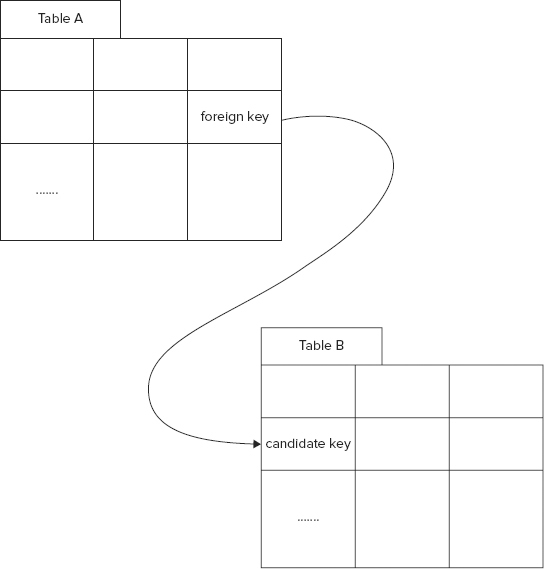
A given value in the foreign key column in Table A (the rightmost, in this particular case) is either null, or it is a link to exactly one row in Table B, the single row that contains the matching value in its leftmost column (again, leftmost in this case).

Most RDBMS engines enforce this relationship, referential integrity, for relations on which it is defined. The enforcement has two parts.

• The first part, enforcing the primary key constraint, guarantees that there is no more than one row in the target table (Table B in Figure 2-3) with the given value as primary key (in its left column in the example). A table may contain, at most, one (possibly multicolumn) primary key. A database that enforces the primary key constraint will fail an attempt to insert a new row into a table if the table already contains the key value found in the new row. For instance, if the table contains three rows with the key column values of “yes”, “no”, and “maybe”, the attempt to add a new row with a key column value of “purple” will succeed. Attempting to add a new row whose key column contains the value “no”, however, will fail.
• The second part of referential integrity enforcement guarantees that if the foreign key is non-null in a row in the child table (Table A in the example), there is a unique record with that key in the parent table (Table B). There are two ways that this rule might be violated, and both are forbidden. An attempt to insert a row with a foreign key whose value is not the primary key of any row in the target table will fail and usually generate an exception. So will the attempt to delete the (unique) row in the parent table that is referenced by a foreign key in the child table. If there is no information in the parent table corresponding to a given row in the child table, that row’s foreign key value must be null.

Transactions

The last of the features frequently supported by RDBMS systems is the transaction. A transaction is a group of operations on the data that must be considered as a unit: They must either all succeed or all fail. Transaction support in a database system is frequently discussed in terms of the extent to which it supports “ACID” properties:

• Atomicity — A transaction is “all or nothing”: Either the entire transaction succeeds or none of it does.
• Consistency — If the database is in a valid state before a transaction, it is still in a valid state after the transaction. A transaction cannot cause the violation of any data constraints.
• Isolation — The state of the database after a transaction is a state that could have been achieved by applying the statements in the transaction serially in some order.
• Durability — Once a transaction has completed, it can’t be forgotten. Even if the power fails or the network collapses, the new state persists until it is changed by other statements.

Database engines frequently allow the data architect fairly fine-grained control over several kinds of transaction support, from permitting access to the data to only one client at a time (slow, but all transactions succeed) to allowing multiple simultaneous access, and failing the entire transaction for a client that, by chance, violates transactional rules (faster but sometimes requires retrying).

Transactions, referential integrity, strong typing, and the relational model are all core concepts of relational data systems. Now that you’ve re-acquainted yourself with them, it is time to turn to the specifics of their use. The canonical language for using relational systems is SQL. As an Enterprise Android developer, you will have to be fluent with SQL both to manage data within the Android platform and to use backend services effectively.

The SQL Language

SQL really is a comparatively simple language. Still, as noted earlier, it is the topic for entire books. A complete description is well outside the scope of this one. Because developers at both ends of a mobile application — the mobile side and the server backend — are likely to use SQL, it is worth taking a few moments to review its main features in general, before turning to the specifics of the SQLite dialect.

Statements in the SQL language can be divided into three large classes, the Data Definition Language (DDL), the Data Manipulation Language (DML), and queries.

Data Definition Language (DDL)

The Data Definition Language (DDL) describes the structure of the data that a database contains. The most common DDL statements are used to define a table — the number of columns it contains, the names of those columns, and the kinds of values allowed in them. This is accomplished with the CREATE TABLE statement, illustrated in Listing 2-1, along with its inverse, DROP TABLE.

LISTING 2-1: The CREATE TABLE statement

DROP TABLE contacts;
CREATE TABLE contacts (
    _id INTEGER PRIMARY KEY AUTOINCREMENT,
    name_raw_contact_id INTEGER REFERENCES raw_contacts(_id),
    photo_id INTEGER REFERENCES data(_id),
    photo_file_id INTEGER REFERENCES photo_files(_id),
    custom_ringtone TEXT,
    send_to_voicemail INTEGER NOT NULL DEFAULT 0,
    times_contacted INTEGER NOT NULL DEFAULT 0,
    last_time_contacted INTEGER,
    starred INTEGER NOT NULL DEFAULT 0,
    has_phone_number INTEGER NOT NULL DEFAULT 0,
    lookup TEXT,
    status_update_id INTEGER REFERENCES data(_id)
);

Listing 2-1 is an example of the definition of a moderately complex table, named contacts. It happens that this is, specifically, the SQLite dialect of SQL, but the definition would look nearly identical in most other dialects. The code creates the single table called contacts with 12 columns, each defined in one line of the code. The name of a table must be unique within a database and is frequently a plural noun, naming the objects found in the rows of the table: EMPLOYEES, NOSES, HIPPOPOTUMUSES, and so on.

The names of the columns in a table must be unique within the table. In the example, the column _id is an integer valued primary key for the table. The AUTOINCREMENT constraint on the _id column causes the db engine to create a new, unique integer for each row, automatically, as it is added.

The other columns in the table use two primitive data types — text and integer. Several of the columns — those that use the REFERENCES keyword — have complex types that are defined in other tables using foreign keys. The column photo_file_id, for instance, is a reference to the table photo_files.

In addition to being able to create tables, SQL DDL allows the creation of other standard RDBMS data structures like views, triggers, and indices. A typical database is likely to contain several tables, maybe an index or two, and depending on the inclinations of the designer, a few triggers or views. The collection of DDL statements that define all of the objects in a given database is called its schema.

Data Manipulation Language (DML)

Data Manipulation Language (DML) statements are used to add, remove, and modify data in the database. There are three DML statements — INSERT, UPDATE, and DELETE. They are all demonstrated in Listing 2-2.

LISTING 2-2: Data Manipulation Language statements

INSERT INTO contacts(
    name_raw_contact_id, photo_id, photo_file_id,
    last_time_contacted, status_update_id)
    VALUES(null, null, null, 1339365417, null);
UPDATE contacts SET starred=1, has_phone_number=1 WHERE _id = 3;
DELETE FROM contacts where _id = 2;

The INSERT statement adds a new row to the table and defines the values in some — in this case, not all — of its columns. The insert will succeed because all of the columns that are required to have values (constrained NOT NULL) have values specified or have defaults (constrained DEFAULT). The primary key for the row inserted by this statement will have an integer value automatically created by the database engine and different from any other value currently in the _id column.

The next statement in Listing 2-2, the UPDATE statement, changes the value of two columns for, at most, one row in the contacts table. It changes the value for the single row in which the value of the primary key is 3. Because the selection criteria is the primary key, there can be, at most, one such row.

The last statement in the listing, the DELETE statement, deletes (in this case) at most one row from the database. Again, this is because the selection criteria is the primary key and there can be at most one record whose primary key is 2. After this statement is executed, there exists no row whose primary key is 2 in the contacts table.

Queries

QUERY is probably the most frequently used of all the SQL statements. In relational terms, the query creates a new relation — a virtual table — that is a restriction of a projection of the cross-product of one or more other tables. Listing 2-3 shows an example of a query that illustrates an INNER JOIN.

LISTING 2-3: Query that uses INNER JOIN

SELECT rc.display_name, c.starred
    FROM contacts c INNER JOIN raw_contacts rc
        ON c.name_raw_contact_id = rc._id
    WHERE NOT rc.display_name IS NULL
    ORDER BY rc.display_name ASC;

As mentioned earlier, a join is an important restriction on the cross-product of two tables. As shown in Figure 2-4, a full cross-product of two tables combines each of the rows from the first table with every row from the second. In the query in Listing 2-3, the table contacts is joined with the table raw_contacts. There are C(contacts) * C(raw_contacts) rows in this cross-product, where C(t) is the number of rows in the table t. This whole cross-product probably isn’t very useful. In the query, though, the ON clause restricts the cross-product to only rows in which the column name_raw_contact_id has the same value as the raw_contacts column _id. The new relation generated by the join contains the rows from contacts, each with the corresponding information from raw_contacts appended. That is definitely useful! The bottom table in Figure 2-4 illustrates a similar join.

By extension it is possible to construct joins of many tables. In RDBMS systems joins are an essential feature in almost the same way that inheritance is an essential feature in object-oriented systems.

This brief review of the SQL language completes the overview of generic relational data storage. All of the discussion in this chapter, so far, applies to both the client and server sides of a distributed mobile application. It is information with which mobile developers may be less familiar than their backend counterparts. Discussing it at such a high level serves not only to help the mobile developer understand an important local tool but also to understand the backend technology that supports her mobile application. It is now time to turn to the specifics of Android’s structured data management tool, SQLite.

INTRODUCTION TO SQLITE

Android uses the open source database engine, SQLite. It is a small, serverless library that has several features that are extremely attractive in the mobile environment. Data stored in SQLite databases on a phone is persistent across processes, through power cycling, and, usually, across upgrades and re-installs of the system software.

SQLite is an independent, self-sustaining project. Originally developed in 2000 by D. Richard Hipp, it quickly filled a niche as a lightweight way to manage structured data. A group of dedicated developers supports a large user community and such high-profile projects as Apple Mail, the Firefox web browser, and Intuit’s TurboTax.

As part of this strong support, each release of SQLite is tested very carefully, especially under failure conditions. The library is designed to handle many kinds of failures gracefully, including low memory, disk errors, and power outages. Reliability is a key feature of SQLite and more than half of the project code is devoted to testing. This is very important on a mobile platform where the environment is less predictable than it is for a device confined to a server room. If something goes wrong — the user removes the battery or a buggy app hogs all available memory — SQLite-managed databases are unlikely to be corrupted and user data is likely safe and recoverable.

The other side of the coin, though, is that SQLite is not really an RDBMS. Several of the features that you’d expect from a relational system, are completely missing. As built for Android, SQLite does support transactions and the SQL language. However, until Android API level 10 (Gingerbread), it did not support referential integrity or strong typing. In more recent versions of Android, SQLite can support referential integrity, but that support is turned off by default. It still does not support strong typing. Its own documentation suggests that one should think of SQLite “not as a replacement for Oracle, but as a replacement for fopen().”

SQLite from the Command Line

Perhaps the best way to introduce SQLite and its vagaries is to use it. In the interests of authenticity, this entire example was recorded on an Android emulator: an Android Virtual Device (AVD). The first line of Listing 2-4 starts an instance of the emulator, using the previously created device configuration named tablet. In this case, that configuration is running Android Ice Cream Sandwich, release 15, v4.0.3. The example would look nearly identical on most other versions of Android or on an actual Android device. For that matter, it would look the same from the command line of any other UNIX-like system that has sqlite3 installed.

A SQLite database is a simple file. On Android devices most applications store their databases in their file system sandbox in a sub-directory named databases. For instance, databases for an application whose package name is com.enterpriseandroid.contacts.webdataContacts are most likely to be in the directory /data/data/com.enterpriseandroid.contacts.webdataContacts/databases. There is no reason, of course, that an application can’t share access to its databases by putting them, instead, into a public storage area (anything stored on the file system named /sdcard, for instance, is publicly available to any application). As you will see in the next chapter, though, there are much better ways to share data than by making the database itself globally available.

The example also demonstrates the use of the adb tool, the Android Debugger, from the Android SDK. adb is the Swiss Army knife of Android tools. It is found in the directory platform-tools of the SDK (which, in the example, is located using the shell variable $ANDROID_HOME). When run, adb connects to a daemon on a running Android system. In this case it is connecting to the emulator started on the line above. To get a shell prompt on the emulator, use the command adb shell.

From the shell prompt, you can run the SQLite command-line utility sqlite3. Listing 2-4 uses the file system sandbox for an installed application whose package name is com.enterpriseandroid.contacts.dbDemo.

LISTING 2-4: Starting sqIite3

wiley> $ANDROID_HOME/sdk/tools/emulator -avd tablet &
wiley> $ANDROID_HOME/sdk/platform-tools/adb shell
# cd /data/data/com.enterpriseandroid.contacts.dbDemo/databases
# sqlite3 demo.db
Enter ".help" for instructions
Enter SQL statements terminated with a ";"
sqlite>

The first thing to remember when using sqlite3 from the command line is that each command must be terminated with a semicolon. Listing 2-5 illustrates this point.

LISTING 2-5: Ending sqlite3 commands with semicolons

sqlite> select * whoops typo
   ...>
   ...> ;
Error: near "whoops": syntax error

Until sqlite3 sees the statement-terminating semicolon, it interprets all input as part of a single SQL statement and offers the continuation prompt, ...>. Only after the semicolon does it parse and evaluate the input, delivering any necessary error messages.

There are also several meta-commands (not part of the SQL language) that are very useful when working with sqlite3. Meta-commands are commands that begin with a period. They are not interpreted as SQL but, instead, as commands to the sqlite3 command-line program. The two most important of these are .help and .exit.

• The .exit command exits the sqlite3 command interpreter.
• The .help command prints a list of other “dot” commands.

SQLite syntax supports a wide variety of data types: TINYINT, BIGINT, FLOAT(7, 3), LONGVARCHAR, SMALLDATETIME, and so on. As mentioned earlier, though, the type of a column is actually little more than a comment. Listing 2-6 demonstrates this by storing the string value "la" into several columns with non-text types.

LISTING 2-6: sqlite3 data types

sqlite> create table test (
   ...> c1 biginteger, c2 smalldatetime, c3 float(9, 3));
sqlite> insert into test values("la", "la", "la");
sqlite> select * from test;
la|la|la

The column type is useful only as a hint to help SQLite choose an efficient internal representation for the data stored in the column. SQLite determines the internal storage type using a handful of simple rules that regulate “type affinity.” These rules are very nearly invisible except as they affect the amount of space that a given dataset occupies on disk.

In practice, many developers just restrict themselves to four primitive internal storage types used by SQLite — integer, real, text, and blob — and explicitly represent timestamps as text and booleans as integers.

There are a number of constraints that can be attached to a column definition. The most important is the PRIMARY KEY constraint. A primary key column contains for each row in a table a unique value that identifies the row.

SQLite does support non-integer primary keys. It even supports composite (multi-column) primary keys. Beware, though, of primary key columns that are not integer primary keys! In addition to implying a unique constraint (described later in this chapter), the primary key constraint should also imply a NOT NULL constraint. Unfortunately, because of an oversight in early versions, SQLite allows NULL as the value of a primary key for any type except integer. Because each NULL is a distinct value (different from even other NULLs) SQLite permits a primary key column to contain multiple NULLs and thus permits multiple rows in a table that cannot be distinguished by their primary key.

As Listing 2-7 demonstrates, an integer primary key column is, by default, also set to autoincrement. That means that SQLite will automatically create a new value for that column for each new row added to the database. To make this behavior explicit, declare the column PRIMARY KEY AUTOINCREMENT.

LISTING 2-7: sqlite3 primary key autoincrement

sqlite> create table test (key integer primary key, val text);
sqlite> insert into test ( val ) values ("something");
sqlite> insert into test ( val ) values ("something else");
sqlite> select * from test;
1|something
2|something else
sqlite>

The autoincrement feature is very useful because through it the database engine itself guarantees that the key created for a new row is unique. However, it presents a problem that can lead to awkward and clumsy code. When adding a new row to the database, the code may have to read the new row immediately after creating it to discover the key that the database assigned.

Another important constraint that might appear in the column definition is FOREIGN KEY. As noted previously, by default, SQLite does not enforce foreign key constraints. Like the column type, it is essentially a comment. This is demonstrated in Listing 2-8.

LISTING 2-8: The foreign key comment

sqlite> create table people (
   ...> name text, address integer references addresses(id));
sqlite> create table addresses (id integer primary key, street text);
sqlite> insert into people values("blake", 99);
sqlite> insert into addresses(street) values ("harpst");
sqlite> select * from people;
blake|99
sqlite> select * from addresses;
1|harpst
sqlite> select * from people, addresses where address = id;
sqlite>

In a database that supported referential integrity, the first insert statement would fail with a foreign key constraint violation. In fact, the attempt to create the table in the first create table statement would fail for the same reason.

Although SQLite does not necessarily enforce referential integrity, the relational concept of a complex type, defined in one table and referenced from others through a foreign key, is central to well designed, easily modified, and efficient data storage. Developers are encouraged to use standard best practices (for example, normalization) when designing SQLite databases. The only difference is that the code accessing the database must be prepared to enforce referential integrity constraints itself instead of depending on the database to do it. Listing 2-9 extends the example begun in Listing 2-8 by demonstrating a simple join.

LISTING 2-9: A simple join

sqlite> insert into addresses(street) values("pleasant");
sqlite> insert into addresses(street) values("western");
sqlite> insert into people values ("catherine", 2);
sqlite> insert into people values ("john", 3);
sqlite> insert into people values ("lenio", 3);
sqlite> select name,street from people, addresses where address = id;
catherine|pleasant
john|western
lenio|western

In this example there is one person who lives on Pleasant Street but there are two who live on Western Avenue. There is, however, only one record in the addresses table for the street named western. The data is not duplicated. The foreign key in the people table refers to the single record that holds the address of the two people who live on Western Avenue.

SQLite supports several other column constraints. They are illustrated in Listing 2-10.

• unique: When this constraint is applied to a column, SQLite will refuse any attempt to add a row to the table that would result in some value appearing in the column more than once.
• not null: When this constraint is applied to a column, SQLite will refuse to perform any operation that would cause the value in the constrained row to be NULL.
• check(expression): When this constraint is applied to a column, the expression is evaluated whenever a new row is added to the table, or when an existing row is modified. If the result of the evaluation is 0 when cast as an integer, the attempt fails and is aborted. If the expression evaluates to NULL or any other non-zero value, the operation succeeds.

LISTING 2-10: Column constraints

sqlite>  create table test (
   ...> c1 text unique, c2 text not null, c3 text check(c3 in ("OK", "dandy")));
sqlite> insert into test values("dandy", "dandy", "dandy");
sqlite> insert into test values("dandy", "dandy", "dandy");
Error: column c1 is not unique
sqlite> insert into test values("dandy", null, "dandy");
Error: test.c2 may not be NULL
sqlite> insert into test values("dandy", "dandy", "bad");
Error: constraint failed
sqlite>

An Example SQLite Database

Now that you’ve explored some of the idiosyncrasies of SQLite, you are ready to work a complete example: a simple contacts database. First create the contacts table:

sqlite> create table contacts (
   ...> _id integer primary key autoincrement,
   ...> name text not null);
sqlite>

The name of the primary key column is determined by an Android system requirement (more about that in the next chapter). Perhaps, after a moment’s consideration, it seems like a great idea to add a column to the table, to record the time at which a contact’s information was last changed. That is accomplished with an additional column and a pair of triggers:

sqlite> alter table contacts add last_modified text;
sqlite> create trigger t_contacts_audit_i
   ...> after insert on contacts begin
   ...> update contacts set last_modified=datetime('now', 'utc')
   ...> where rowid = new.rowid;
   ...> end;
sqlite> create trigger t_contacts_audit_u
   ...> after update on contacts begin
   ...> update contacts set last_modified=datetime('now', 'utc')
   ...> where rowid = new.rowid;
   ...> end;
sqlite>

Now try adding a record to verify that things are working so far:

sqlite> insert into contacts(name) values("Dianne");
sqlite> select * from contacts;
1|Dianne|2012-06-30 08:29:18
sqlite>

Perfect! The contacts need addresses. You can create a table for those:

sqlite> create table addresses(
   ...> _id integer primary key autoincrement,
   ...> number integer not null,
   ...> unit text,
   ...> street text not null,
   ...> city integer references cities);
sqlite>

As noted previously, if referential integrity support had been enabled, this table definition would cause an error because the cities table does not exist. In SQLite’s default configuration, however, it is not a problem: You can define it later.

What’s missing is a way to connect contacts to their addresses. In order to do that, you need one more table:

sqlite> create table contact_addresses(
   ...> contact integer references contacts,
   ...> address integer references addresses);
sqlite>

You can now add data:

sqlite> insert into contacts(name) values("Guy");
sqlite> insert into contacts(name) values("Chet");
sqlite> insert into contacts(name) values("Tim");
sqlite> insert into addresses(number, street)
   ...> values(651, "North 34th Street");
sqlite> insert into addresses(number, street)
   ...> values(345, "Spear Street");
sqlite> insert into addresses(number, street)
   ...> values(1600, "Amphitheatre Parkway");
sqlite> select * from contacts;
1|Dianne|2012-06-30 09:46:42
2|Guy|2012-06-30 09:46:42
3|Chet|2012-06-30 09:46:42
4|Tim|2012-06-30 09:46:42
sqlite> select * from addresses;
1|651||North 34th Street|
2|345||Spear Street|
3|1600||Amphitheatre Parkway|
sqlite> insert into  contact_addresses(contact, address) values(1,1);
sqlite> insert into  contact_addresses(contact, address) values(2,2);
sqlite> insert into  contact_addresses(contact, address) values(3,3);
sqlite> insert into  contact_addresses(contact, address) values(4,2);
sqlite>

The contacts now have addresses. You can see those addresses using a join query:

sqlite> select name, number, street
   ...> from contacts, addresses, contact_addresses
   ...> where contacts._id = contact_addresses.contact
   ...> and addresses._id = contact_addresses.address;
Dianne|651|North 34th Street
Guy|345|Spear Street
Chet|1600|Amphitheatre Parkway
Tim|345|Spear Street
sqlite>

Perhaps you would like to determine how many contacts are to be found at each address. That can be done using the count function and the group by clause:

sqlite> select count(name), number, street
   ...> from contacts, addresses, contact_addresses
   ...> where contacts._id = contact_addresses.contact
   ...> and addresses._id = contact_addresses.address
   ...> group by number, street;
2|345|Spear Street
1|651|North 34th Street
1|1600|Amphitheatre Parkway
sqlite>

Perhaps, now that you know how many contacts are at each address, you want to show a new list of contacts ordered by their address. In a small database like this, that is no problem. On the other hand, if there are a lot of addresses and you are going to use the address number and street as a sort key, you should probably create an index. An index simply optimizes the process of finding a specific value in the indexed columns. It does this at the expense of the space needed to store the index and the time needed to update it on write operations. Columns (or sets of columns) that don’t change often and are frequently used as selection or sort criteria are good candidates for indices. You can now create indices on both contacts’ names and addresses.

sqlite> create index t_contacts_name on contacts(name);
sqlite> create index t_addresses_num_street on addresses(number,street);
sqlite>

Take a look at that list of contacts again, this time organized by address:

sqlite> select number, street, name
   ...> from contacts, addresses, contact_addresses
   ...> where contacts._id = contact_addresses.contact
   ...> and addresses._id = contact_addresses.address
   ...> order by number asc, street desc, name asc;
345|Spear Street|Guy
345|Spear Street|Tim
651|North 34th Street|Dianne
1600|Amphitheatre Parkway|Chet
sqlite>

Suppose that one of the contacts moves to a new address. Perhaps you want to keep track of your contacts’ current addresses, as well as their previous ones. You might do that by adding a new column to the contact_addresses table, called moved_in, to record the date on which a contact arrives at a particular address.

...> alter table contact_addresses add moved_in text;
sqlite>

Notice that the type of the new field to be used as a timestamp is text. The standard way to represent a timestamp in SQLite is as a text field within which times are represented by fixed format strings.

This code places a default value for the move in date into all of the records already in the database:

sqlite> update contact_addresses set moved_in=datetime(0, 'unixepoch'),
sqlite> select * from contact_addresses;
1|1|1970-01-01 00:00:00
2|2|1970-01-01 00:00:00
3|3|1970-01-01 00:00:00
4|2|1970-01-01 00:00:00
sqlite>

Now you can move the contact Guy from Spear Street to Amphitheatre Parkway:

sqlite> insert into contact_addresses(contact, address, moved_in)
   ...> values(2, 3, datetime("2012-05-01"));
sqlite> select * from contact_addresses order by contact desc, moved_in asc;
4|2|1970-01-01 00:00:00
3|3|1970-01-01 00:00:00
2|2|1970-01-01 00:00:00
2|3|2012-05-01 00:00:00
1|1|1970-01-01 00:00:00
sqlite>

Notice that there are now two records in the contact_addresses table for contact 2, one much more recent than the other. A query similar to the last will show all of Guy’s addresses:

sqlite> select name, number, street, moved_in
   ...> from contacts, addresses, contact_addresses
   ...> where contacts._id = contact_addresses.contact
   ...> and addresses._id = contact_addresses.address
   ...> order by name asc, moved_in desc;
Chet|1600|Amphitheatre Parkway|1970-01-01 00:00:00
Dianne|651|North 34th Street|1970-01-01 00:00:00
Guy|1600|Amphitheatre Parkway|2012-05-01 00:00:00
Guy|345|Spear Street|1970-01-01 00:00:00
Tim|345|Spear Street|1970-01-01 00:00:00
sqlite>

Using the having clause, you can show only contacts that have moved at least once:

sqlite> select name, number, street
   ...> from contacts, addresses, contact_addresses
   ...> where contacts._id = contact_addresses.contact
   ...> and addresses._id = contact_addresses.address
   ...> group by name
   ...> having count(contacts._id) > 1
   ...> order by name desc;
Guy|1600|Amphitheatre Parkway
sqlite>

And, finally, with a sub-select, you can show only each contact’s most recent address:

sqlite> select name, number, street
   ...> from contacts, addresses, contact_addresses
   ...> where contacts._id = contact_addresses.contact
   ...> and addresses._id = contact_addresses.address
   ...> and moved_in = (
   ...> select max(moved_in)
   ...> from contact_addresses
   ...> where contact = contacts._id)
   ...> order by name desc;
Tim|345|Spear Street
Guy|1600|Amphitheatre Parkway
Dianne|651|North 34th Street
Chet|1600|Amphitheatre Parkway

At this point, the database schema looks like this:

sqlite> .schema
CREATE TABLE addresses(
_id integer primary key autoincrement,
number integer not null,
unit text,
street text not null,
city integer references cities);
CREATE TABLE contact_addresses(
contact integer references contacts,
address integer references addresses,
moved_in text);
CREATE TABLE contacts (
_id integer primary key autoincrement,
name text not null, last_modified text);
CREATE INDEX t_addresses_num_street on addresses(number, street);
CREATE INDEX t_contacts_name on contacts(name);
CREATE TRIGGER contacts_audit_i
after insert on contacts begin
update contacts set last_modified=datetime('now', 'utc')
where rowid = new.rowid;
end;
CREATE TRIGGER contacts_audit_u
after update on contacts begin
update contacts set last_modified=datetime('now', 'utc')
where rowid = new.rowid;
end;
sqlite>

Although simple, this example demonstrates many of the concepts used in even very complex databases. The next chapter shows you how to harness these concepts in an Android application.

SUMMARY

In the first half of this chapter, you reviewed some of the essential concepts that underlie relational database systems:

• Relations (tables), cross-products (joins), projections, and restrictions
• The SQL language: data definition, manipulation, and queries
• Transactions, data typing, and referential integrity

Many of these concepts will be familiar to experienced enterprise system developers. Android, however, is among the first platforms to bring them to a mobile environment and they may be new even to very experienced mobile systems developers.

In the second half of this chapter you met SQLite, Android’s mechanism for storing structured data. While SQLite speaks SQL, it is not at all the kind of RDBMS with which most enterprise developers are familiar. Rather, it is a library included in an application that allows the application to efficiently and safely manage structured data stored in a file. However, its support for data typing and referential integrity is limited.