
Assessment of Revenue Potentials of Ancillary Service Provision by Flexible Unit Portfolios
Stephan Koch ETH Zurich, Power Systems Laboratory, Physikstrasse 3, 8092 Zurich, Switzerland
Abstract
In this chapter, an economic evaluation of frequency control provision (primary and secondary control) by flexible unit portfolios, also referred to as virtual power plants (VPPs), is presented. VPPs consist of generators, energy-storage units, and controllable thermal loads. This investigation uses the previously developed power nodes modeling framework (PNMF). Time simulations over parameter ranges are undertaken so as to determine the control potential provided by two benchmark portfolios. Ancillary service market data from Switzerland are used to assess the value of using energy-storing units for frequency control instead of generators only. This yields a quantitative evaluation of the commercial potential of control services by coordinated flexible unit portfolios. Furthermore, an approach for sharing the profit among the various participating actors is presented by taking advantage of the e3value methodology for modeling value exchanges between actors in a market setting.
1 Introduction and Literature Review
A key application of virtual power plants (VPPs) in power systems is the provision of frequency control reserves. A crucial question for this use case is the revenue that can be achieved with a certain amount of control capacity provision on ancillary service markets. Previous work on the value of controllable demand has been done mainly for the cases of load shifting and the exploitation of price differences, such as in [1]. The value of energy-storage devices for short-term dispatch and balancing was also assessed in the literature, e.g., in [2]. Frequency control ancillary service provision by plug-in hybrid electric vehicles (PHEVs) was described and economically evaluated in [3], demonstrating substantial revenue potentials.
In this chapter, we examine a market-based approach to ancillary service provision by flexible unit portfolios consisting of storage, controllable load, and generation units. In this setup, individual market players, called aggregators, control unit populations in a suitable way for delivering control reserves. The aggregators can both be separated from or integrated in established electricity utilities. The main point of investigation is the contribution that a certain type of unit can make to a control product. This requires a consideration of the inherent energy constraints that any kind of storage unit exhibits (acceptable internal temperature range in the case of thermal loads). This question is approached similarly to [4] by a time-simulation setup using benchmark portfolios. Here, we use the power nodes modeling framework (PNMF) first presented in [5] and [6]. The results of the time-domain simulations are merged with an analysis of historical price data, in this case of the Swiss frequency control reserves market, in order to estimate the financial revenue potential of a certain unit-portfolio bidding into the market.
The results of this chapter are partly based on [7] and have also been reported in [8], Chapter 7. This chapter is structured as follows: Section 2 discusses properties of liberalized electricity markets and the role of aggregators. In Section 3, the modeling of the revenue from ancillary service provision by flexible unit portfolios is presented. Section 4 presents a case study using the benchmark portfolios 3 and 4 from [8], Chapter 6. Section 5 presents the modeling of a method for profit sharing between the various actors. Section 6 presents concluding remarks. The used notation is summarized in Table 2.1.
Table 2.1
Notation for this chapter
| Var. | Unit | Meaning | Var. | Unit | Meaning |
| C | [EUR] | Cost | α | [-] | Storage share |
| E | [MWh] | Energy | β | [-] | Admin-fee coeff. |
| K | [-] | No. of time steps | γ | [-] | Control resp-fee coeff. |
| k | [-] | Time step | δ | [-] | Storage-fee coeff. |
| M | [-] | Mapping | Δ | [-] | Change |
| n | [-] | Number | Π | [EUR] | Profit |
| R | [EUR] | Revenue | π | Price | |
| T | [-] | Time span | |||
| Subscript | Meaning | Subscript | Meaning | ||
| act | Actors/activities | ICT | Inf. and. Comm. Tech. | ||
| activ | Activities | MTU | Market Time Unit | ||
| actor | Market actor | net | Net value | ||
| bat | Battery | opp | Opportunity | ||
| capa | Capacity | prov | Provision | ||
| en | Energy | ramp | Ramping | ||
| exch | Exchanges | s | Sampling | ||
| fuel | Generator fuel | spot | Spot market | ||
| gen | Generator | strg | Storage | ||
| Superscript | Meaning | Superscript | Meaning | ||
| base | Base case value | feed-in | Feed-in of energy | ||
| bat | Battery | fixed | Fixed one-time fee | ||
| capped | Value with upper bound | floored | Value with lower bound | ||
| CL | Controllable loads | gen | Generation | ||
| cons | Consumption | max | Maximum | ||

2 Aggregators in Electricity Markets
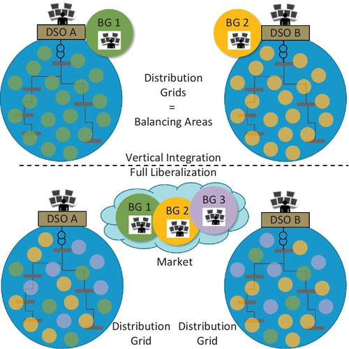
In the “old world” of vertically integrated electricity utilities, the tasks of electricity generation, network operation, and supplying final customers were usually carried out by the same company. The simultaneous fulfillment of several roles enabled the company to perform a joint optimization of their generation and network assets. This is not possible in the same way in liberalized electricity systems. Depending on the regulatory framework, the distribution system operators (DSOs) may need to accommodate various electricity suppliers in their grid domain, while suppliers may be active in more than one distribution grid. Figure 2.1 illustrates the change from a vertically integrated utility structure to a liberalized electricity system. The exchange of energy between producers and suppliers is handled via an electricity market, and the generation companies have to bid control reserves and other grid services into ancillary service markets administrated by the transmission system operator (TSO). The information exchange between grid operators and market players is usually restricted in order to guarantee non-discriminatory conditions. This has a number of implications for the introduction of “SmartGrid” functionalities in power systems, which we will briefly discuss in the following.
2.1 The Role of Aggregators
Aggregators are relatively new entities in electricity systems that possess the ability to influence a number of grid-connected units via a suitable communication interface. The units are coordinated, usually by a centralized optimization, in order to fulfill a certain control goal as a group. Aggregators may operate in different parts of the electricity network and utilize the units in their portfolio for trading in electricity and ancillary service markets. Note that, depending on the market design, an aggregator can also be understood as an entity that coordinates the units in a certain area of the network in the sense of a MicroGrid (MG) [9], but we do not consider this setting here. We use the term aggregator synonymously to VPP operator.
Aggregators are market players by nature. Their aim is the commercially successful operation of their connected units, be it in the form of energy-schedule optimization or in the form of power-system control services. They can both be separated from or associated with an established electricity utility. The control actions that they impose on the connected power-system units may influence the load flows as well as transformer and line loadings of one or several distribution systems. Thus, care has to be taken if relevant distribution-grid constraints exist in the area of operation of an aggregator.
2.2 Distribution-Grid Constraints
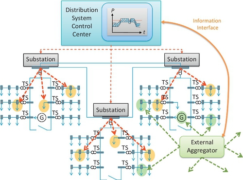
The existence of grid constraints is a self-evident fact for any distribution system. Although traditionally distribution grids were designed such that the peak load could be comfortably accommodated without running the risk of transformer or line/cable overloading, coordinated control actions on large amounts of flexible demand may quickly drive the system towards the constraints. For example, negative tertiary control provided by electric water heaters, called by the TSO during the evening peak, is likely to increase the peak load to an unacceptable level. In the long run, structured information interfaces must be established between the DSOs and the aggregators that control the flexible demand in their area. Figure 2.2 outlines this situation. The interface can be established, e.g., in the form of time-varying power ranges that denote the permissible change in power consumption by the flexible load.
2.3 Unit-Monitoring Challenges
Another complication of ancillary service provision by coordinated dispersed units is the need to prove to the TSO that the power delivery actually happened as requested. For instance, the relevant documents for the Swiss power system [10] stipulate that all units providing secondary control reserves have to deliver continuous online measurements to the TSO. In the case of generation units, this requires expensive instrumentation and telemetry. When a large number of dispersed units is delivering the same service, this degree of online monitoring may be difficult to achieve. Consequently, it may be necessary to adapt the regulatory framework of ancillary service provision depending on the nature of the control resources.
3 Modeling of Revenue Potential
The profitability of the application of load flexibility for power-system control purposes depends, among other factors, on the design of the underlying electricity market, specifically on wholesale energy and ancillary service markets. While most of today's wholesale markets are tailored for international electricity trading, ancillary service markets remain largely in the national domain. This implies that there is a large amount of diversity among the ancillary service market structures between countries. Reference [11] presents a comprehensive overview on different ancillary service market structures and nomenclatures. For instance, the reserve delivery times and specifications of control service quality are widely different. As an example, we use the Swiss market design as described in [12] as a basis for the evaluation of ancillary service provision. In other market settings, the regulatory framework used for revenue generation may be entirely different, so the methodology used here may have to be adapted in order to yield meaningful results.
The Swiss control reserves market is based on an auctioning system with a pay-as-bid pricing method [13] for primary, secondary, and tertiary control reserves. Bids can be entered online and are accepted or rejected by the TSO, who represents the only source of demand in these markets according to the calculated control-reserve requirements for the control area. The auction result is not disclosed in detail, but the average price of the most expensive accepted 20 MW is published by Swissgrid [14].
The financial compensation for primary and secondary control is outlined below. Note that, due to the national nature of the ancillary service market, the capacity prices are issued in Swiss Franc (CHF). Since the energy price is based on the SwissIX spot market price of the European Power Exchange (EPEX) [15], it is issued in Euro (EUR).
3.1 Regulatory Basis for Revenue Calculation
Revenue of Primary Control Primary control is compensated by a capacity fee per MW of control band provided for a certain time span. Bids can only be placed symmetrically (equal control band for positive and negative deviation from the working point). Currently, auctions take place once a week. Energy compensation is not used since system-frequency deviation is relatively symmetrical and does not exhibit longer deviations from zero. The prices for primary control capacity in 2011 are depicted in Figure 2.3 (a).

Revenue of Secondary Control In the Swiss ancillary service market, secondary frequency control is compensated by a capacity fee and an energy fee. While the capacity price per MW of control band provided for a certain time span is determined by the auction process, the energy price follows a fixed scheme: the control energy is averaged over a time slice of 15 minutes and paid for with an hourly spot market price including a bonus of ± 20%. In the case of a generation increase (or load decrease), the ancillary service provider receives the spot price + 20%; in the case of a generation decrease (or load increase) he pays the spot price −20%. In order to smoothen price spikes, the provider’s revenues are floored by the weekly base price and his costs are capped by the weekly base price. The prices for secondary control capacity in the year 2011 are presented in Figure 2.3 (b). The energy prices based on the spot market prices are depicted in Figure 2.3 (c).
Capacity Price Assumption For the analysis of revenue potentials and the profitability of ancillary service provision by flexible unit portfolios, we consider the average price as depicted in Figure 2.3 for the primary and secondary control capacity. This is an idealistic assumption, since in a pay-as-bid auction, perfect bidding (placement of the bid at the clearing price) is needed to achieve this result. The calculations consequently serve as a performance benchmark, not necessarily as a realistic prediction of achievable revenues. For reasons of comparability, we convert the prices from CHF to EUR. We assume a conversion factor of 1.25 CHF/EUR.
3.2 Net-Operating Profit
Based on the market design presented above, we evaluate the maximum net profit that can be made (under the idealistic assumption of perfect bidding) by using a combined portfolio of power nodes to provide ancillary services. To calculate the operating profit Π [EUR], we use the following formula:
where Rcapa [EUR] is the capacity revenue of the ancillary service provision, Ren,net [EUR] is the net control energy revenue, Cstrg [EUR] is the storage cycling cost, Cramp [EUR] is the ramping cost of the generator, ΔCfuel [EUR] is the change in fuel cost through the ancillary service provision compared to a constant setpoint, and Copp [EUR] is the opportunity cost incurred by not using the generator control band for energy production. The individual revenue and cost terms are defined as follows:
with the control reserve capacity price ![]() the duration of reserve provision Tprov [h], and the provided symmetrical power control band of width Pprov [MW]. The following term describes the energy revenue (secondary control):
the duration of reserve provision Tprov [h], and the provided symmetrical power control band of width Pprov [MW]. The following term describes the energy revenue (secondary control):
with the capped and floored spot prices πspotcapped and πspotfloored and with the fed-in or consumed control energy (netted over market time units kMTU = 1,…, Kmtu of 15 minutes) Enetfeed - in and Enetcons Describing the storage cycling cost for all time steps k = 1,…, K is straight forward:

where ![]() [MMWh] is the marginal battery storage cost and ts is the sampling time of the problem. The generator ramping cost is equal to
[MMWh] is the marginal battery storage cost and ts is the sampling time of the problem. The generator ramping cost is equal to

where ![]() is the marginal ramping cost. The change in fuel cost, depending on the fuel price
is the marginal ramping cost. The change in fuel cost, depending on the fuel price ![]() is equal to
is equal to

The opportunity cost incurred by the generator represents the financial loss associated with reserving the control band in the generator's operating range. Let α ∈ [0,1] be the share of the control band that is covered by the energy-storing unit (battery, thermal load). As depicted in Figure 1.4, we consider the financial loss due to two effects: first, the reduction of the possible energy production range to the upside (by the positive control band) when the wholesale market price is higher than the fuel cost and the generator wants to produce at maximum power; and second, the forced production of energy (by the negative control band) when the market price is lower than the fuel cost and the generator wants to produce at minimum power. These two effects are mapped into an opportunity cost function that reads
For each time step, the energy portion (1 – α) ts Pprov that either could have been produced for a profit (when πspot (k) > πfuel (k)) or that had to be produced for a loss (when πspot (k) < πfuel (k)) is summed up. Note that this kind of modeling constitutes a certain simplification of reality. To be exact, one would have to perform a unit commitment and economic dispatch of the power plant with and without the reserved control band, the difference of which constitutes the opportunity cost. In that way, start-up/shut-down and ramping can be considered. Since this would introduce an additional dependency on individual parameters of the power plant, we opt for the presented simplified approach. Note that another slight error is introduced in the ramping cost since it is quadratic and up- and down-ramping for working point changes would have to be superposed on the ramping caused by ancillary service provision. However, we do not deem this effect crucial for this study and consequently neglect it.
4 Simulation Study
In the following, we conduct a simulation study to evaluate the frequency control approach using the benchmark portfolios A (generator and battery) and B (generator and water heater population). We define simulation scenarios that shall enable an illustration and evaluation of the benefits arising from using energy storage for ancillary services.
4.1 Simulation Scenarios
In order to quantify the benefits of energy storage for primary and secondary frequency control, we take the following approach: Real system frequency and secondary frequency control signal data (available in 10-second resolution over a time span of 30 days) are scaled to a benchmark control band of Pprov = ± 10 MW. This is a realistic bid size in many ancillary service markets and is useful for easy comparison. We will simulate the system over a time span of 30 days with variations in power and energy capacity of the units. In particular, we are interested in the share of the control band that an energy-storing unit (storage device or thermal load) can securely account for, which provides a measure for the value of using the combination of units instead of the generator alone. The following parameters are varied: 1) the share α of the control band that is covered by the energy-storing unit (defining its rated power), while the generator control band is scaled to 1 – α, and 2) the storage capacity of the energy-storing unit, measured in hours of charging at rated power disregarding the efficiency.
The simulation scenario parameter sets are described in Table 2.2. The battery-storage capacity is sized simply according to the desired duration of charging at maximum power. For the water-heater population, a more detailed approach is necessary: since the water heater control band shall be symmetrical (up- and down-regulation of the power consumption equally possible), the autonomous energy demand of the water heaters must be taken into account. In most cases, water heaters have a relatively low capacity factor (average power demand divided by rated power). The symmetry of the control band is achieved by selecting the working point such that the mean value of energy demand is consumed when the control signal is equal to zero. The daily draw profile is scaled such that 75% of the water contained in the tank is drawn during one day. These facts imply that for a larger storage capacity fewer water heaters are needed since the energy demand is higher. Figure 2.5 depicts the number of water heaters over the parameter ranges.
Table 2.2
Parameter variations for frequency control assessment
| Battery | Water heater | |
| Storage share (α [%]) Energy cap. C/Δuloadmax[h] |
[10:10:90] [1, 2.5, 5, 7.5, 10] |
[10:10:90] [3:1:8] |


We present the most important economic parameters for the case study in Table 2.3. The cost function coefficients are defined in accordance with the portfolio definitions in [8], Chapter 6. We carry out all simulations with a prediction horizon of N = 2 (time step of 10 s), which enables honoring inter-temporal and state constraints while acknowledging that control signals are hardly predictable over longer time horizons.
4.2 Numerical Results
We conduct the parameter variations described above in order to assess the value of the joint reserve provision. The following quantities are of interest for the performance evaluation:
a) deviation from the control signal (in the form of root mean square error (RMSE), normalized to the size of the control band);
b) mean storage state of charge (SOC) level deviation from the working point;
c) mean storage power deviation from the working point;
d) mean generator power deviation from the working point;
e) cost incurred by the portfolio operation and revenue earned by the ancillary service provision;
f) net profit from the portfolio deviation;
g) net profit change (compared to ancillary service provision by generator only); and
h) net profit per MW of battery storage per individual water heater.
Primary Control with Portfolio A
The provision of primary control reserves with Portfolio A (Battery + Generator) is depicted in Figure 2.6. The battery share is varied between 10% and 90% of the control band, and the battery capacity is varied between 1 an 10 h. The parts a) to h) of the figure show:
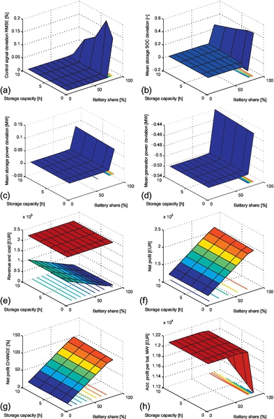
a) The control-signal deviation is non-zero only for battery shares above 80%. Even then, the deviation stays small with a maximum of about 0.17%. This is due to the fact that the maximum-frequency deviation rarely exceeds ± 100 mHz, so only about half of the control band is utilized. The battery-storage capacity does not have a have a strong impact on the control-signal deviation, which also holds true for all other variables discussed below.
b) The mean SOC deviation from the scheduled working point is equal to zero below 70% = 80% since the storage is hardly used for the reserve provision. Above this storage-share level, the battery storage operates mostly in its upper SOC region.
c) The mean storage-power deviation becomes positive for a control-band share above 80% as well, which corresponds to the increased mean SOC. Below 80%, it is equal to zero.
d) The mean generator-power deviation is constantly equal to about–0.525 MW for power shares below 80%. This is due to the negative bias of the control signal, which is entirely accommodated by the generator. Above a level of 80%, the generator produces slightly more on average.
e) The totally incurred cost for the 30 days of operation (lower surface) ranges from about EUR 100,000 down to about zero. This is due to the decrease in opportunity cost as well as the negative bias of the control signal. The revenue (upper surface, from capacity bidding only since the control energy is not compensated in primary control) is constant at about EUR 220,000.
f) The net profit slopes up from about EUR 120,000 to almost EUR 220,000 along with a change from 10% to 90% of battery share.
g) The net-profit change with respect to the base case (generator only) ranges from about 15 up to about 100%.
h) The net profit per MW of battery power is equal to about EUR 12,000 for the considered 30 days of operation for battery shares below 70%. Exceeding this share reduces the profit due to the increased cycling of the battery storage.
Primary Control with Portfolio B
Figure 2.7 shows the aggregated simulation results of primary control provision with Portfolio B (Battery + Electric Water Heaters). As before, we vary the storage share between 10% and 90%. The energy capacity is varied from 3 to 8 hours for a symmetrical control band. The parts a) to h) of the figure show:
a) The control-signal deviation starts at a storage share of about 50%. Below this level, the portfolio is able to fulfill the control task perfectly. The discrepancy to the results of Portfolio A can be explained by the fact that the water-draw profile induces a variation of the SOC even if the control signal was equal to zero.
b) The average SOC deviation (from a base value of 0.6) is equal to 0.4 for small water-heater shares. This is due to the fact that the optimizer chooses to move the SOC to that region in the beginning of the time simulation. The average SOC drops to about 0.1 for a share of about 60% and then rises again to almost 0.3 when the water heater share attains 90%. This behavior is relatively arbitrary and largely depends upon the decision-variable penalization and control-signal time series.
c) The average storage-power deviation fluctuates between about 0.1 MW for storage shares of 10% and slightly above 0.8 MW for 90% and small energy capacity. This also depends on the decision-variable penalties and control-signal time series.
d) The average generator power deviation follows the same shape as the mean storage-power deviation and fluctuates between about–0.45 MW and + 0.3 MW.
e) The totally incurred cost is equal to about EUR 100,000 for a storage share of 10% and slopes down to about 15,000 for 90%. The revenue generated is constant over the entire parameter span and is equal to about EUR 220,000.
f) The net profit varies – consequently – from about EUR 120,000 to EUR 205,000 as the storage share increases.
g) The net profit change with respect to the base case (generator only) has a similar shape and varies between about 15% and 95%.
h) The net profit per water heater varies between about EUR 4 and EUR 15 for the considered 30 days of operation. The slightly counter-intuitive result of increasing returns for a larger storage capacity is due to the number of water heaters decreasing in this direction of the parameter variation (see Figure 1.5).
Secondary Control with Portfolio A
Figure 2.8 presents the provision of secondary control with Portfolio A (Battery + Generator). The battery power share and energy capacity are varied in the same way as before. We observe the following details in the simulation results:

a) The control signal deviation is only equal to zero for small battery shares. This is due to the fact that the energy contained in the secondary control signal quite easily exceeds the available storage capacity. Unlike primary control, a secondary control signal usually exhibits frequent attainment of positive and negative extremes, which implies the full activation of the available reserves.
b) The average SOC deviation ranges between about 0.1 and 0.4. The maximum values are attained on a ridge-like curve in the vicinity of the diagonal of the parameter space.
c) The mean storage-power deviation is close to zero for small storage shares and attains increasingly higher values of up to 0.5 as the storage share increases to 90%. The storage utilization does not change significantly with the storage capacity.
d) The mean generator-power deviation largely follows the same shape with a relatively constant offset. It varies between about −0.8 and −0.2, being slightly steeper than the surface in c) for large storage shares.
e) The totally incurred cost ranges between about EUR 90,000 to approximately EUR 45,000. Note that the slope of the surface in the battery-share direction becomes positive again for battery shares above 60% to 70%. This is due to the increased storage cycling. The attained revenue is constant at about EUR 220,000.
f) The net profit consequently varies between a minimum of EUR 130,000 and a maximum of about EUR 175,000.
g) The net-profit change with respect to the base case (generator only) varies between about 10% to almost 55%.
h) The net profit per MW of storage power is equal to almost EUR 12,000 for small storage shares and slopes down to about EUR 5,000 as the share increases. This indicates a decreasing marginal value of replacing generation capacity control band with energy storage since the actual utilization of the storage causes cycling cost and energy losses.
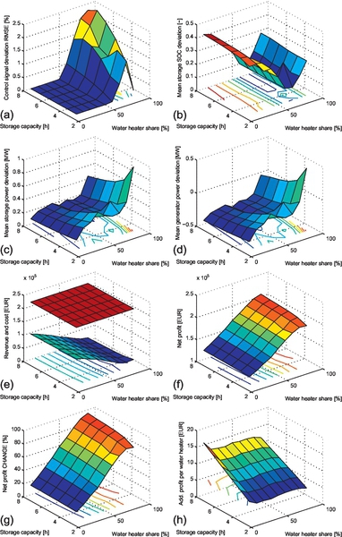
Secondary Control with Portfolio B
Figure 2.9 presents the provision of secondary control with Portfolio B (Generator + Electric Water Heaters). The following observations can be made in part a) – h) of the figure:

a) The control-signal deviation remains close to zero for all water-heater shares below 80 – 90%. The non-zero values for 8 hours of storage capacity and a storage share of about 70% can be regarded as a random event.
b) The average SOC deviation is approximately v-shaped in the direction of increasing storage shares. It is close to zero for small storage shares and slopes downwards to about −0.2 for a storage share of around 60%. Above that, the average SOC slopes up again to a maximum of about 0.2.
c) The mean storage-power deviation has a similar shape, being close to zero for small storage shares, negative at about −0.3 MW for a storage share of about 60%, and positive at about 0.35 MW for a storage share of 90%.
d) The mean generator power deviation exhibits the same shape as c) with a relatively constant offset of about −0.8 MW.
e) The totally incurred cost in EUR slopes downward in the direction of the storage share, starting at EUR 95,000 down to slightly below zero for a storage share of 90%. The negative cost is due to the change in fuel cost induced by the reserve provision along with a lack of storage cycling cost.
f) The net profit consequently ranges from about EUR 125,000 to EUR 220,000 between small and large storage shares.
g) The net-profit change with respect to the base case (generator only) ranges between 15% and about 85%.
h) The net profit per water heater ranges from about EUR 5 to EUR 14 for the 30 days of operation, depending on the parameter set. The explanation for the upward slope in the direction of the storage capacity is as explained as for the case “Primary Control with Portfolio B.”
5 Profit-Sharing Methodology
Having derived the attainable operating profit by two flexible benchmark portfolios, we proceed with the development of a methodology for sharing the profit between different players in the market system. For the representation of the considered market environment, we take advantage of a modeling methodology named e3value [16]. It serves to create so-called business value models that allow the description of exchange processes of services and financial compensations between various entities according to a certain market design. It has been successfully applied to the modeling of distributed generation (DG) business cases [17] and other business fields. In the context of the present work, modeling activities with the e3value methodology have been carried out in [18]. The purpose of this modeling is, in our case, the structured representation and illustration of the exchanges between the aggregator and its surroundings, and, in the case of privately owned thermal loads, the final customers.
We will only briefly introduce the e3value and refer the interested reader to [16]. At its core, the methodology consists of a (graphic and mathematical) representation of actors, their various business activities, and the exchanges between them. This enables the calculation of the profitability for each of the actors. The methodology comprises the following principal elements, which are also depicted in Figure 2.10:
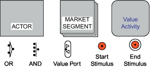
Actor: An actor is an entity in the market that pursues certain goals by conducting business-related value activities.
Value Activity: A value activity is a set of business-related actions that generates a revenue or incurs a cost for a certain actor.
Value Port: A value port is a connector that enables a value exchange (i.e., exchange of certain goods/services/money) between different actors. These exchanges are associated with specific value activities.
Start Stimulus: A start stimulus is a principal need or desire of an actor for a certain good or service, which creates a demand and a chain of value exchanges.
End Stimulus: An end stimulus is the end of a value exchange chain.
AND and OR gates: These are routing elements that create logical relations between exchanges and enable the merging of exchange paths.
5.1 Business Value Model
The business value model of the ancillary service provision by an aggregator is depicted in Figure 2.11. We will introduce the various actors, activities, and exchanges in the following. Note that the present model only considers exchanges that are influenced by the ancillary service provision. A detailed analysis and parameterization of the base case (electricity system without the aggregator) as carried out in [18] is omitted here for shortness. For this reason, we also omit the modeling of the DSO since we do not consider the effects of the aggregator’s business on the distribution system in this study.

5.2 Actors and Activities
The following actors and activities are considered in the model:
Transmission System Operator (TSO): The TSO is responsible for controlling and operating the transmission grid (usually comprising the voltage levels of 220 kV and 380 kV in Europe). This includes monitoring and control of the current grid topology (position of breakers and switches within the grid) and the voltage in all parts of the transmission grid. The principal activity of interest for our analysis is the contracting of ancillary service providers by determining the required control reserve capacity, administrating the auction process for the reserve tendering, and also calling the reserves when needed. The ancillary services are paid for by grid users via grid usage fees levied by the TSO.
Aggregator (Agg): The Aggregator is a novel entity in the power system that operates between the TSO, Power Plants, Electricity Supplier, and Final Customer. It contracts both generation capacity and final customers in cooperation with the electricity suppliers in order to deliver ancillary services to the TSO.
Power Plant (PP): The power plant produces and sells electricity via the wholesale electricity market. It also delivers ancillary services, in our case frequency control reserves, to the TSO. A bilateral contractual relation with the Aggregator serves to integrate a generator control band into the portfolio administrated by the Aggregator.
Electricity Supplier (Supp): The Electricity Supplier serves the final customer with electricity at a certain price. The contract modalities can be arbitrarily defined and usually consist of a certain base price, an energy price per kWh of used electricity, and in the case of large customers also a power capacity fee per kW of peak load. The electricity is usually bought on the electricity market or via bilateral contracts. Note that the electricity supply is not depicted in Figure 1.11 since it is not influenced by the Aggregator’s business model. The relevant activity for our analysis is Allowing Load Aggregation, which means that the Electricity Supplier consents and collaborates with the aggregator in contracting flexible loads of final customers. This can include offering a demand response (DR) tariff to the final customers, the financial benefits of which are enabled by the Aggregator’s business.
Wholesale Market (WhMa): The Wholesale Market is an electricity exchange where trading with other market actors takes place. As the other actors are not modeled, the Wholesale Market serves as a source of revenue generation.
Equipment and ICT Supplier (ICT): The Equipment and ICT Supplier delivers the necessary equipment and Information and Communication Technology (ICT) to the Aggregator.
Final Customer (Cust): The Final Customer contracts an Electricity Supplier for the supply with electric energy. The relevant activity is the response to a control signal sent by the Aggregator, which is compensated by a response fee.
Storage Owner (StrgOw): The Storage Owner possesses and operates an energy-storage device (in our case, a battery) that the Aggregator includes in his portfolio. The Storage Owner gets compensated by a fee for his services to the Aggregator.
5.3 Exchanges
Now the value exchanges between the actors are described and quantified. We refer to the net-operating profit calculation presented in Section 3.2 and make use of the simulation results from Section 4. A number of degrees of freedom exist, which call for assumptions and/or business model design decisions. We will outline one possible variant to design the value exchanges. In order to calculate the cash in- and outflows of the actors, we will consolidate the exchanges for the different activities and actors. The following exchanges take place:
Aggregator Capacity Fee (AggCapFee): The capacity fee earned by the aggregator is equal to the overall capacity revenue earned by the portfolio described by (2):
Aggregator Energy Fee (AggEnFee): Similarly, the energy fee is equal to the total net energy revenue according to (4):
Power-Plant Capacity Fee (PPCapFee): We assume that, in the base case, the power plant offers 100% of its control capacity band (in our case ± 10 MW) to the ancillary service market. In our considered business model, we assume that the generator does not bid directly into the ancillary service market anymore. The generator share of the control band (1 – α) is instead provided to the Aggregator, and the remaining share, a, is used for energy production for the Wholesale Market. This means that the power plant does not earn a capacity fee anymore. Compared to the base case (α = 0) where it used to earn Rcapa, the revenue is the negative of the original capacity fee:
Power-Plant Energy Fee (PPEnFee): The same is true for the energy fee:
Control-Service Compensation (CtrlServComp): The control service compensation is an internal flow within the aggregator. It is equal to the revenue earned by the ancillary service provision:
Generation-Coupling Fee (GenCoupFee): The generation-coupling fee shall compensate the provision of control capacity by the power plant. We dimension the fee such that the power plant does not incur any profit or loss with respect to bidding its capacity into the market. The main incentive for the power plant to participate in the proposed scheme is the reduction of its ramping activity, which allows for a longer equipment life in thermal power plants. We use the aggregator’s control capacity and energy revenues as a basis and deduct the reduction in opportunity cost (with respect to the base case) due to using the control band share α for energy production. We also adjust for changes in fuel cost with respect to the base case. Note that further adjustments may have to be made for the changes in the power plant’s control energy revenue, which we neglect here for simplicity. Consequently, the generation-coupling fee is defined as follows:
Administration Fee (AdminFee): In order to incentivize the participation of the electricity supplier (only relevant for Portfolio B) and to cover costs incurred by the need to communicate with the customers, we propose the following administration fee as a percentage β of the Aggregator’s revenue that can be attributed to the storage share α:

Wholesale Electricity Fee (WhElecFee): The wholesale electricity fee is defined as the storage control band share α times the opportunity cost incurred in the base case Coppbase:
The rationale behind this is that a share α of the control band is now utilized for energy production instead of ancillary service provision, so the opportunity cost is reduced by this amount.
Equipment and ICT Cost (EquipICTFee): The equipment and ICT cost is incurred for the communication and control infrastructure in a centralized control center (CICTfixed) and on the premises of the final customers (nCLCICTCL, where nCL is the number of final customers) or, respectively, on the premises of the storage owner (CICTbat):

Control Response Fee (CrtlRespFee): This fee is paid by the Aggregator to the final customers as a compensation for offering their controllable load capacity. We base the fee on the Aggregator’s revenue, multiplied by the storage share α and another modifier γ:

Storage Fee (StrgFee): The storage fee compensates the operation of the energy-storage device. We define it as the cycling cost plus the generator’s opportunity cost reduction αCoppbase, modified by a factor δ:

5.4 Cash-Flow Consolidation
In accordance with Figure 2.11, we enumerate the actors, activities, and exchanges in the form of column vectors, which is practical for a mathematical representation of the exchanges and the attribution of cash flows to the activities and actors. The following vectors are defined:


In our case, the dimensions of the vectors are nactor = 8, nactiv = 10, and nexch = 11. The cash-flow consolidation is performed by a linear mapping between actors, activities, and exchanges. We introduce the mapping matrices, Mexch (nactiv × nexch) which maps the exchanges to the activities, and Mact (nactor × nactiv) which maps the activities to the actors:
In Mexch, we denote an inflow of money into a value activity with + 1 and the outflow out of a value activity with −1. Unrelated exchange/activity combinations get a 0. In Mact, we assign a 1 to an activity pertaining to an actor and a 0 to unrelated activity/actor combinations. According to Figure 1.11, the matrices are defined as follows:


Note that the columns of Mexch must sum to zero since every exchange makes a positive contribution to exactly one activity and a negative contribution to another. The columns of Mact must sum to one since every activity is associated with exactly one actor. We calculate the financial in- and out-flow CashInOut to and from each actor by applying the presented linear maps to the vector of financial exchanges CashExch:
5.5 Application Example
In order to demonstrate the application of the profit-sharing methodology, we consider one example for each of the four simulated scenarios. For each portfolio, we take one data point with a relatively high net operating profit from the parameter scans described in Table 2.2. For both Portfolio A and B, we select a storage share of 60% (α = 0.6) and a storage capacity of 5 h; in the case of water heaters, this corresponds to 8,955 units in the population, which means that one water heater contributes on average ± 670 W of controllable power. We approximate the results for one year by multiplying the revenue earned during the 30 simulated days by 365/30. The following (exemplary) numerical values were selected for the exchange parameters: β = 0.02, γ = 0.4, δ = 0.775, CICTfixed = 10, 000 EUR, CICTbat = 10, 000 EUR, and CICTCL = 10 EUR.
Table 2.4 presents the financial results for the chosen scenarios as obtained from the simulations presented in Section 4. We will briefly discuss the results with respect to the differences between the scenarios.
Table 2.4
Yearly financial results of the four selected scenarios
| Quantity Value in [EUR] | Prim. A | Prim. B | Sec. A | Sec. B |
| Rcapa | 2,628,000 | 2,628,000 | 2,628,000 | 2,628,000 |
| Ren,net | 0 | 0 | –68,985 | –68,985 |
| Cstrg − Cstrgbase | 30 | 0 | 100,980 | 0 |
| Cramp − Crampbase | –23 | –60,306 | –4,000 | –12,116 |
| ΔCfuel − ΔCfuelbase | –19 | 2,032 | 46,095 | 6,281 |
| Copp − Coppbase | –879,167 | –879,167 | –879,167 | –879,167 |
| Π – Πbase | 879,179 | 937,441 | 736,092 | 885,003 |
| Π – Πbase per water heater | – | 104.68 | – | 98.83 |
| Π – Πbase per battery MW | 146,529 | – | 122,682 | – |
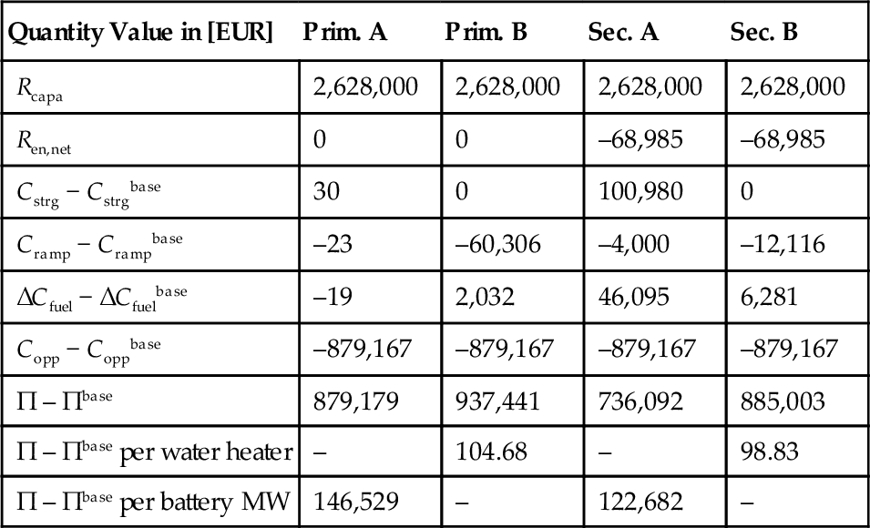
• Prim. A (Primary control provision by Portfolio A): This scenario is characterized by the dominance of the generation unit in following the control signal, while the battery storage serves as a backup that is only used when needed. This is due to the control signal being small enough to be covered almost always by the generator and due to the cycling cost incurred by the storage. Changes in ramping cost, cycling cost, and fuel cost are small.
• Prim. B (Primary control provision by Portfolio B): The contribution of the water heaters is more significant here, since water heaters incur no cycling cost but are able to smooth the control signal, which in turn saves ramping cost for the generator.
• Sec. A (Secondary control provision by Portfolio A): Here, the battery storage is needed more often for control-signal tracking, which incurs cycling cost and also drives the generator fuel cost up. Note that the energy revenue from secondary control is negative, which is due to the negative bias of the control signal and is compensated by fuel cost savings with respect to the case of not providing reserves at all (not presented in this table).
• Sec. B (Secondary control provision by Portfolio B): In this scenario, the control signal is smoothed by the water heaters, so less ramping cost is incurred. The fuel cost is driven by a small increase in thermal losses in the water heaters.
Table 2.5 presents the monetary exchanges between the actors in numerical form, which is also visualized graphically in Figure 2.12. It can be seen that, for our parameterization of the value exchanges, there is a win-win situation for the participating actors. The additional monetary inflow into the system arises due to the fact that the power plant can use its generation capacity for energy production and sales on the market, as opposed to reserving the control band for ancillary service provision. This is depicted by a negative bar for the actor “Energy Exchange,” which obviously is to be interpreted as the source of additional revenue, not a financial loss incurred by the energy exchange.
Table 2.5
Cash in-/out-flows in the four selected scenarios
| Actor / Value in [EUR] | Prim. A | Prim. B | Sec. A | Sec. B |
| Transmission System Operator | 0 | 0 | 0 | 0 |
| Aggregator | 123,418 | 115,329 | 123,418 | 128,465 |
| Power Plant | 46,095 | 2,032 | 46,095 | 6,281 |
| Supplier | 0 | 31,536 | 0 | 30,708 |
| Wholesale Market | –879,167 | –879,167 | –879,167 | –879,167 |
| ICT Provider | 20,000 | 99,550 | 20,000 | 99,550 |
| Final Customer | 0 | 630,720 | 0 | 614,164 |
| Storage Owner | 689,655 | 0 | 689,655 | 0 |
| Sum | 0 | 0 | 0 | 0 |
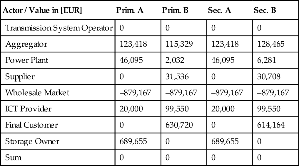

For Portfolio A, most of the additional revenue is going to the storage owner (about EUR 690,000). The economic viability of operating the battery for this kind of revenue largely depends on the cost structure of the technology and the considered business model (ownership of the storage, buying or renting, combined use cases, etc.). At the present cost of about US$ 1,500 per kW of installed power [19] (amounting to US$ 9 million for a 6 MW battery), the economic viability may be questionable, but prices are expected to decrease steeply in the future and multi-objective utilizations of the battery can be considered. Details on this question are beyond the scope of this thesis. Furthermore, the ICT supplier earns a flat fee of EUR 10,000 for the control-center equipment and another EUR 10,000 for the on-site equipment. The aggregator generates a revenue of about EUR 123,000.
For Portfolio B, the additional revenue is distributed between the final customers (about EUR 631,000 for primary and EUR 614,000 for secondary control), the electricity supplier (about EUR 31,000), the ICT equipment supplier (about EUR 100,000), and the aggregator (about EUR 115,000 for primary and EUR 128,000 for secondary control).
The amount of money transferred to the final customers corresponds to EUR 70.43 (CHF 88.04 with our assumed exchange rate) for primary control and EUR 68.58 (CHF 85.73) for secondary control per year for a single water heater. In relation to the total cost of electricity of an exemplary household consuming 5,000 kWh per year at CHF 0.14/kWh (average price) with an assumed monthly base fee of CHF 10.00, this amounts to 10.5% to 10.7% of the electricity bill. Note that we assume an unchanged electricity cost for the water heater operation, which may imply that cost differences induced by time-variable tariffs have to be compensated by the electricity utility, which in turn requires a redistribution of the profits generated by the ancillary service provision.
If this financial compensation is sufficient for incentivizing, customer participation will largely depend upon the customers’ motivation or reluctance to engage in a novel utilization of their domestic appliances which might have noticeable effects on the appliance, behavior (e.g., by additional ON and OFF switchings during the day). The trust that the customers have in their electricity suppliers and in novel players in the electricity market is therefore a major factor for successful implementation. By means of a suitable marketing strategy (such as pointing out the advantages of a “SmartGrid” for the transition toward a clean energy supply), an adoption of the proposed scheme may be achieved.
6 Concluding Remarks
We discussed the integration of flexible portfolios consisting of controllable loads and storage devices in conjunction with generation units into frequency control structures. A business value model including a methodology for sharing the profits between different actors based on the e3value framework was created and parameterized for the control reserve provision by a flexible unit portfolio administered by an aggregator. The optimization-based control strategy derived in [8], Chapter 6, proved to be useful for distributing the control actions in an economically optimal way on the participating units while honoring state constraints of storage devices. We find that the simulation-based sizing of the storage units for frequency control is a promising approach since it takes into account time-series properties, such as the energy contained in the control signal, as well as the duration of deviations from zero.
The simulated scenarios show that the combination of generators and energy-storing units yields a substantial net operating-revenue increase that may be used to amortize the investment in the joint portfolio. For a real deployment of the described control systems, further investigations of the storage-level management over time, accurate modeling of battery degradation, and ancillary service bidding strategies are necessary. Furthermore, the simplifying assumptions in this work should be addressed in future research. For instance, the market prices of both ancillary service and wholesale markets are assumed to be unaffected by the additional ancillary service provision by the aggregator. While this is realistic for a small and unique aggregator in a large system, the widespread implementation of such systems will have an impact on the overall market liquidity and price structure. The opportunity cost incurred by the generator should also be subject to further investigations.