
Simple Dynamic Models in Time-Series Data
Having learned about heteroscedasticity, Touro was wondering what particular problems could occur with time-series data. Prof. Metric commends him for a good question and says that we will discuss these problems in this chapter and will be able to:
1. Detect the autocorrelation in time-series data and master the corrections;
2. Analyze the autoregressive models and applications;
3. Explain other dynamic models and perform the relevant tests;
4. Apply Excel into estimating the models learned in (1), (2), and (3).
Prof. Metric says that dynamic models examine the continuous impact of any change over more than one period. We will examine the effect in three ways: lag values of the error, lag values of the dependent variables, and lag values of the explanatory variables.
Autocorrelation
Prof. Metric says that a static model for time-series data contains only variables of the contemporaneous period for all explanatory and dependent variables. In this case, if all classic assumptions are also satisfied, then regression of time-series data is similar to that of cross-sectional data; that is, OLS produces BLUE results. Thus, this static model does not need any correction before running a regression, and the simple-regression model is written as:
![]()
where Cov(et, ez) = 0 for t ≠ z.
![]()
where Cov(et,ez) = 0 for t ≠ z.
Prof. Metric reminds us that we already had hands-on experience in Chapter 3 performing a regression of EXPSt on RGDPt and EXCHAt.
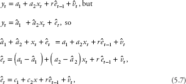
However, if the classic assumption (iv) for time series Cov(et,ez) = 0 for t ≠ z is violated even when all explanatory and dependent variables are in the current period—that is, Cov(et,ez) ≠ 0 for t ≠ z—then we have a dynamic model with lag values of the error, and the problem is called autocorrelation or serial correlation. Given equation (5.1), the autocorrelation equations with one lag error and k lag errors are written respectively as:
![]()
![]()
Combining equation (5.3a) or equation (5.3b) with equation (5.1) yields the following model for one lag error or k lag errors, respectively:
![]()
![]()
In equations (5.4a) and (5.4b), vt has a constant variance
![]() and cov(vt, vz) = 0; t ≠ z.
and cov(vt, vz) = 0; t ≠ z.
We also assume that all series are stationary, |rk| < 1 for k = 1, 2,…, k.
In addition, it can be shown that
![]()
Hence, et is also homoscedastic.
However, the covariance of et and et−k is not homoscedastic. Specifically, it can be shown that
![]()
From these results, the population correlation function is:
![]()
Since (5.4a) has only one lag value of the errors, k = 1, and corr(et,et-1) = r.
Equations (5.4a) and (5.4b) and (5.5) tell us that there are certain relations between the error terms of two or more periods, so the model has an autocorrelation problem.
Prof. Metric says that the two consequences of the autocorrelation are similar to those of heteroscedasticity:
(i) The standard errors are incorrect, so statistical inferences are not reliable.
(ii) The OLS estimator is still unbiased, but it is no longer the BLUE, so it is possible to find an alternative estimator with a lower variance.
Also, similar to heteroscedasticity, the correction for each problem will be discussed separately in the next section.
Detecting Autocorrelation
We learn that we can examine an autocorrelation function or carry out an LM test to detect autocorrelation.
Autocorrelation Function
The series rk, where k = 1, 2,…, k, is called the autocorrelation function or the correlogram of the errors. This function reveals the correlation between the errors that are two periods apart through k periods apart. The estimated correlation function, which is a sample version of equation (5.5) is:
Thus, we can perform a regression of equation (5.2), obtain the residual ȇt, and generate thee lag values of ȇt so that we can calculate each ![]() . We then compare this
. We then compare this ![]() with the ratio ±1.96 / T1/2, similar to equation (1.15). The value ±1.96 is the 95 percent bounds of a standard normal distribution, and T is the sample size. We will reject the null hypothesis of no autocorrelation if
with the ratio ±1.96 / T1/2, similar to equation (1.15). The value ±1.96 is the 95 percent bounds of a standard normal distribution, and T is the sample size. We will reject the null hypothesis of no autocorrelation if
![]()
In this case, one or more lag error terms are correlated to the current error term, implying that the autocorrelation problem exists.
Booka asks, “Why do we have to use t = k+1 in equation (5.6)?” Taila offers an explanation,
Once we obtain the residual êt from regression, we need to generate its lag values. For example, if you want to test the model in equation (5.4a), then k = 1. In this case, we need to generate et−1 and will lose the first observation. Hence, the sum in equation (5.6) will start from t = 2 because k +1 = 1 + 1= 2. For k = 2, the sum will have to start from t = 3, and so on.
Prof. Metric is very pleased with Taila’s explanation and says that we will have a chance to practice this method in the Exercises section. Most econometric software programs provide a graph of the correlogram with the bounds ± 1.96 / T1/2, called the 95 percent Bartlett Band, superimposed on the graph so that we do not have to calculate it by hand. The terminology “Barlett Band” comes from a seminal work on this subject by Bartlett (1946). For Excel, we will have to buy an Add-in tool called NumXL, so Prof. Metric does not require us to draw this graph.
LM Test
We focus on the case with one lag error first. The empirical version of equation (5.4a) contains êt−1 and ![]() :
:
where c1 = a1 − ![]() and c2 = a2 −
and c2 = a2 − ![]() ,
,
Hence, the procedure for performing the LM test for (5.4a) is as follows.
Estimate the model equation (5.1): yt = a1 + a2 + et.
Obtain êt and generate êt-1
Estimate equation (5.7) and obtain R2 for the four-step LM test:
(i) H0: r = 0; Ha: r ≠ 0.
(ii) Calculate LMSTAT = T*R2.
(iii) Find ![]() using either a chi-square distribution table or Excel. Note that J is the degree of freedom and equals the number of restrictions; in this case J = 1 because we only have to test one lag value for et−1.
using either a chi-square distribution table or Excel. Note that J is the degree of freedom and equals the number of restrictions; in this case J = 1 because we only have to test one lag value for et−1.
(iv) If ![]() we reject the null hypothesis, meaning r is different from zero and implying that autocorrelation exists.
we reject the null hypothesis, meaning r is different from zero and implying that autocorrelation exists.
Next, Prof. Metric gives us an example, “Suppose estimating the model in equation (5.7) yields R2 = 0.205, and the sample size T = 24, then what is the test results?”
We work on the test as follows:
(i) H0: r = 0; Ha: r ≠ 0.
(ii) Calculate LMSTAT = T*R2 = 24*0.205 = 4.92.
(iii) Find ![]() : we try both a chi-square distribution table and Excel, and find that
: we try both a chi-square distribution table and Excel, and find that ![]() = 3.84.
= 3.84.
(iv) Since ![]() , we reject the null hypothesis, meaning r is different from zero and implying that autocorrelation exists.
, we reject the null hypothesis, meaning r is different from zero and implying that autocorrelation exists.
Prof. Metric says that the test can be extended to equation (5.4b) in the same manner except that J will be equal to the number of lag errors that need to be tested.
Correcting Autocorrelation
(i) The standard errors are incorrect
Similar to the case of heteroscedasticity, OLS can be used to estimate the coefficients when autocorrelation is present, and then corrected standard errors are computed. The corrected standard errors are called the heteroscedasticity and autocorrelation consistent (HAC) or Newey-West standard errors. The concept of HAC standard errors is similar to that of White’s standard errors introduced in the previous chapter.
Nevertheless, Newey-West standard errors are superior to White’s standard errors in two regards: first, they correct for both problems, heteroskedasticity and autocorrelation; second, they are consistent for autocorrelated errors in all forms and so do not require a specification of a dynamic error model as in the case of the heteroscedasticity problem. Ignoring autocorrelation often leads to overstating the reliability of the OLS estimates.
For example, estimating a model with autocorrelation yields the following results:
y1 = 4.74 + 2.48xt; R2 = 0.88; T = 56.
(se) (2.37) (1.02) incorrect standard error
(se) (3.65) (1.97) correct standard error
Hence, the t-tests using incorrect standard errors give significant coefficient estimates while the correct ones yield insignificant ones.
(ii) The OLS estimator is no longer the BLUE
Although the corrected standard errors can be obtained, we learn that it is preferable to use another form of the GLS models to obtain an estimator that is BLUE when an autocorrelation problem exists. Given the following model:
yt = a1 + a2xt + et and et = ret−1 + v1, we have
yt = a1 + a2xt + ret−1 + v1.
Retrogress backward one period:
yt−1 = a1 + a2xt−1 + êt−1,
so
êt−1 = yt−1 − a1 − a2xt
yt = a1 + a2xt + r(yt−1 − a1 − a2xt−1) + vt
= a1 + a2xt + ryt−1 − ra1 − ra2xt−1 + vt
yt = a1(1 − r) + a2xt + ryt−1 − a2rxt−1 + vt
yt − ryt−1 = a1(1 − r) + a2xt − rxt−1 + vt.
Hence, we can estimate the following model:
![]()
where ![]() = yt − ryt−1,
= yt − ryt−1, ![]() = 1 − r,
= 1 − r, ![]() = xt − rxt−1.
= xt − rxt−1.
Prof. Metric reminds us to use the “Constant is Zero” or “No Constant” command in any econometric package, because ![]() is no longer a constant. Estimating model (5.8) will yield BLUE results because the serially correlated error, et, is substituted out. In practice, r is nonexistent, and we need the estimated autocorrelation coefficient of the errors
is no longer a constant. Estimating model (5.8) will yield BLUE results because the serially correlated error, et, is substituted out. In practice, r is nonexistent, and we need the estimated autocorrelation coefficient of the errors ![]() in equation (5.6).
in equation (5.6).
He also reminds us that the predicted values are for ![]() = yt − ryt−1, so we need to calculate the predicted value of y:
= yt − ryt−1, so we need to calculate the predicted value of y:
![]()
where yt−1 is the actual value of y at period (t − 1), and ![]() can be calculated using the formula in equation (5.6).
can be calculated using the formula in equation (5.6).
Autoregressive Models
We now move to the autoregressive (AR) model, which contains the lag dependent variables instead of the lag values of the error term. Prof. Metric says that this model requires special time-series analyses, because it involves only the dependent variable and its own lags instead of the addition of any external explanatory variable.
The Model
A dependent variable in an AR model can contain many lag values. Hence, the model can be denoted as AR(n) where n is the number of lag dependent variables, and the model is called the AR of order n. A model is called an autoregressive model of order one if the dependent variable is correlated to its first lag only. This model is denoted as AR(1) and can be written as:
![]()
If the coefficient estimate |a| < 1, then the series gradually approaches zero when the time, t, approaches infinity, and is said to be stationary. When |a| ≥ 1, the series is said to be nonstationary. If |a| >1, then the series explodes as t approaches infinity. If |a| = 1, then the series keeps winding aimlessly upward and downward with no real pattern and so is said to follow a random walk. In this case, equation (5.9) becomes:
![]()
The model in equation (5.10) is called a “random walk,” because the movement of the series is so random that the best you can guess about what happens in the next period is to look at the result in the current period and then add some random error to it. This behavior is in fact illustrated in equation (5.10).
Prof. Metric says that et is still assumed to be an independent random variable with a mean of zero and a constant variance. He also says that if all lag variables are stationary as in equation (5.9) and there is no autocorrelation, then the OLS estimation produces BLUE results. For example, a model with one constant and two lag values can be estimated using the OLS technique and is written as:
![]()
Point Prediction
Booka offers an example from her company: estimating a stationary AR(1) model of the demand for econometrics books gives the following results:
DEMANDt = 69 + 0.9 DEMANDt−1.
Demand value for last year is DEMANDt−1 = 480 volumes. Thus, we calculate the demand for this year as:
DEMANDt = 69 + 0.9*480 = 501 (volumes).
This process can be extended into the future and is called “recursion by the law of iterated projections” (the recursive principle for short). The proof is provided in Hamilton (1994).
Interval Prediction
The formula for the standard error of the prediction se(p) with T as the sample size is shown in Hill, Griffiths, and Lim (2011) as:
![]()
Prof. Metric gives us an example of SSE = 120 and T = 32. He tells us to use these hypothetical values in calculating the interval prediction for this year.
We start with the point prediction of 501. The standard error of the prediction is:
![]()
Next, we decide to choose a 95 percent confidence interval. Typing =TINV(0.05, 30) into an Excel cell gives us tC = t(0.975, 30) = 2.042. Finally, we calculate the interval prediction as:
DEMANDt = 501 ± 2*2.042 = (497; 505).
Thus, this year Booka will need to order between 497 and 505 volumes of econometrics books. We think it might be best to play it safe and follow the upper bound of 505 volumes.
First-Difference Model
Prof. Metric tells us that if a series follows a random walk, we might end up with a spurious regression, which produces significant regression results, but from completely unrelated data. There are two cases that need to be addressed separately. The first case is addressed in this section because it involves only lag dependent variables. The second case will be discussed in section 3 because it involves external lag variables.
If one of the lag dependent variables is unit coefficient (ak = 1), then taking the first difference of the equation can turn it into a stationary series of a first-difference model. For example, taking the first difference of equation (5.10) yields the following model:
![]()
Δyt is a stationary series because et is an independent random variable with a mean of zero and a constant variance; there is no aimless factor in it. Any series that can be made stationary by taking the first difference (e.g., yt in equation (5.10)) is said to be integrated of order one, which is denoted as an I(1) with the letter I standing for “integrated.” The stationary model obtained by taking the first difference (e.g., Δyt in equation (5.12)) is said to be integrated of order zero and is denoted as an I(0).
This characteristic can be extended to estimating an AR(n) model, in which (n − 1) series are stationary—for example, an AR(2) model that has the first lag series nonstationary:
![]()
We can take the first difference of yt to obtain the following model:
![]()
Since the series becomes stationary, this equation can be estimated using the OLS technique.
We then have hands-on experience with an I(0) model. Touro offers an equation for the values of his tour-package sales:
ΔSALEt = SALEt − SALEt−1 = 0.11 * SALEt−2.
Data on sale values for the previous years are: SALEt−1 = $4,400 and SALEt−2 = $4,600.
ΔSALEt = 0.11 * 4,600 = $506.
We work on the problem and are able to calculate the predicted sale value for this year as:
SALEt = ΔSALEt + SALEt−1 = $506 + $4,400 = $4,906.
Prof. Metric tells us that an I(1) series is also called a first-difference stationary series.
Other Simple Dynamic Models
We learn that this section only discusses other dynamic models under the assumption that all series are stationary. More in-depth discussions of nonstationarity will be offered in the later chapters.
Distributed lag (DL) models contain lag values of explanatory variables in addition to the lag dependent variables. If all classic assumptions are satisfied, then OLS can be performed.
A general DL model is written as:
![]()
For example, if spending on nondurable goods (SPEND) depends on wage (WAGE) of current period and the past period, then the model is:
SPENDt = 30 + 0.3 * WAGEt + 0.2 * WAGEt−1.
Suppose monthly data for WAGEt = $2,800 and WAGEt−1 = $3,000, then the predicted value can be calculated as:
SPENDt = 30 + 0.3 * 2,800 + 0.2 * 3,000 = 30 + 840 + 600 = 1,470
Interval prediction can be calculated using the formula for the standard error of the prediction in equation (5.11).
Autoregressive Distributed Lag Models
Another model, which includes lagged dependent variables in addition to other explanatory variables, is called the autoregressive distributed lag (ARDL) model. Again, if all classic assumptions are observed, then OLS can be performed. For example:
![]()
Suppose WAGEt−1 = $3,000 and SPENDt−1 = $2,000 for previous month, then a prediction can be obtained:
SPENDt = 60 + 0.4 * 3000 + 0.4 * 2000 = 60 + 1,200 + 800 = 2,060
We learn that a general ARDL should have lagged values of the dependent variables in addition to current and lagged values of the other explanatory variables. The model is written as follows:
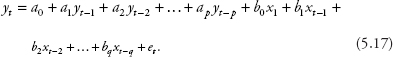
That is, if we use the notation ARDL(p, q) for the model, then p represents the number of lagged y’s, and q represents the number of lagged x’s. For example, an ARDL(1, 2) is called an ARDL of order (1,2) and is written as:
![]()
In this case, we will lose two data points when we generate the data for our regressions (in fact, we only lose one observation for y but two observations for x, so we still have to eliminate the first two rows in the dataset). Note that we also lose five degrees of freedom performing any hypothetical test on the model in equation (5.18).
To decide how many lag values we should include in an ARDL model, we should make sure that there is no omitted variable by checking on the statistical significance of coefficient estimates. Other than that, we should use fewest numbers of lags that eliminates serial correlation. Including too many lag values will increase the number of irrelevant variables and inflate the variances of coefficient estimates.
Data Analyses
Prof. Empirie tells us that we will apply Excel estimation to most of the models learned in the theoretical sections: models with lag values of the error (autocorrelation), models with lag dependent variables (AR models), those with lag values of the explanatory variables (DL models), and unit root test for all three models. However, Excel is not the ideal software to perform a Box-Jenkins procedure, so we will skip this procedure.
Testing Autocorrelation
The file Ch05.xls., Fig 5.1 contains data on salary (SAL) and spending (SPEND). We notice that Prof. Empirie has also copied and pasted SAL in column A into column E for our convenience in a later regression. First, we regress SPEND on SAL:
Click on Data and then Data Analysis on the ribbon.
Select Regression, then click OK.
Enter B1:B34 in the Input Y Range box.
Enter A1:A34 in the Input X Range box.
Choose Labels and Residuals.
Check the Output Range button and enter G1.
Click OK then OK again to override the data range.
Copy and paste the residuals (et) into column C.
Generate et−1 by copying and pasting cells C2 through C34 into cells D3 through D35.
Copy and paste SAL in column A into column E (here the action has already been done by Prof. Empirie).
Next, we regress the Residuals et on et−1 and SAL.
Click Data and then Data Analysis on the ribbon. Select Regression, then click OK.
For Input Y Range: enter B3:B34.
For Input X Range: enter D3:E34.
Uncheck the box Labels—that is, do not use Labels.
Check the Output Range button and enter Q1.
Click OK and then OK again to override the data range.
Figure 5.1 shows sections of this second regression with the number of observations and R2.
From this figure, T = 32 and R2 = 0.79, so LMSTAT = 32*0.79 = 25.28. Typing =CHIINV(0.05,1) into any cell gives you ![]() = 3.84. Since LMSTAT >
= 3.84. Since LMSTAT > ![]() , we reject the null hypothesis, meaning r is different from zero and implying that autocorrelation exists.
, we reject the null hypothesis, meaning r is different from zero and implying that autocorrelation exists.
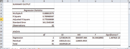
Figure 5.1 T and R2 for autocorrelation test
Prof. Empirie points out to us that we always use R2 instead of adjusted R2 even when the model has more than one explanatory variable. This is also true for the heteroscedasticity tests in Chapter 4 because we wish to play safe and avoid missing the borderline cases.
Regressing with Autocorrelation
Prof. Empirie tells us that the first four columns of the file Ch05.xls. Fig.5.2 are the same as those in the file Ch05.xls.Fig.5.1. The commands for this section will continue from that step.
In cell E3 type =C3^2, then press Enter.
Copy and paste the formula into cells E4 through E34.
In cell F3 type =C3*D3, then press Enter.
Copy and paste the formula into cells F4 through F34.
In cell E35 type =SUM(E3:E34), then press Enter.
Copy and paste the formula into cells F35.
In cell G3 type =F35/E35, then press Enter.
Copy and Paste Special the value in cell G3 into cells G4 through G34.
Copy and paste the values in cells B2 through B34 into cells H3 through H35.
Copy and paste the values in cells A2 through A34 into cells I3 through I35.
In cell J3 type =B3 − (G3*H3), then press Enter (this is SPEND*).
Copy and paste the formula into cells J4 through J34.
In cell K3 type =1 − G3, then press Enter (this is X1*).
Copy and paste the formula into cells K4 through K34.
In cell L3 type =A3 − (G3*I3), then press Enter (this is SAL*).
Copy and paste the formula into cells L4 through L34.
Next, we need to regress SPEND* on X1* and SAL*.
Go to Data Analysis and choose Regression, then click OK.
In the Input Y Range box enter J2:J34.
In the Input X Range box enter K2:L34.
Check the box Labels, Constant is Zero, and Residuals.
Check the Output Range button and enter P1.
Click OK then OK again to obtain the results.
Figure 5.2 reports the regression results.
From this figure, the estimated equation is:
SPEND*t = 3015.65 X1*t−1 + 0.0009 SAL*t−1;
(se) (170.355) (0.00271)
Adjusted R2 = 0.9087; T = 32.
Because SPEND* = SPENDt − rSPENDt−1, to obtain predicted values of SPENDt:
Copy and paste the values in cells Q26 through Q57 into cells M3 through M34.
In cell N3 type = M3+G3*H3, then press Enter.
Copy and paste the formula into cells N4 through N34.
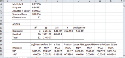
Figure 5.2 Regressing with autocorrelation: The results
We learn that we can calculate interval prediction as usual.
Invo has collected data on the Singapore-Australia real exchange rate (EXCHA) and exports from Australia to Singapore (EXPS) in millions of dollars. The data are available in the file Ch05.xls.Fig. 5.3. We proceed to regress EXPSt on EXCHAt−1:
Click on Data and then Data Analysis on the ribbon.
Select Regression in the list, then click OK.
A dialog box appears.
Enter B1:B33 n the Input Y Range box.
Enter C1:C33 in the Input X Range box.
Choose Labels and Residuals.
Check the Output Range button and enter E1.
Click OK then OK again to overwrite the data.
The results of the estimated coefficients are displayed in Figure 5.3.
In the data file, the predicted value of EXPS2013 is in cell F56. The value can be verified by this equation:
EXPS2013 = −9929.6148 + 4807.4210 EXCHA2012
= −9929.6148 + 4807.4210* 6.98 ≈ 23,626 (in millions of dollars).
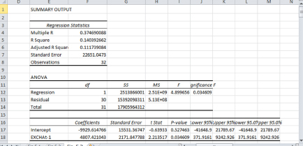
Figure 5.3 DL model: Regression results
Prof. Empirie says that the estimation procedure for an ARDL model is a combination of an AR model estimation and a DL estimation; thus, there is no need to discuss in detail in the class.
Exercises
1. The file Energy.xls contains data on energy demand in Hawaii. Estimate the AR(1) model by regressing energy period t on energy period t−1.
2. Obtain the interval prediction using the results in Question 1 and a handheld calculator.
3. Given the information in Table 5.1, use a hand calculator to compute the sample correlation of êt with êt−1 and êt−2, then make a decision on the autocorrelation problem.
Table 5.1 Residuals from an OLS estimation with sample size T = 4
t |
1 |
2 |
3 |
4 |
êt |
−0.18 |
0.4 |
−0.34 |
0.045 |