
4
Syntax Sphere
4.1. Basic syntactic concepts
4.1.1. Delimitation of the field of syntax
Syntax is a key branch of linguistics. It focuses on the scientific study of the structure of the sentence as an independent unit. The word order, the dependency relationships between these words and, in some languages, the relationships of agreement as well as the case marking, are among the points that attract the attention of most of the researchers. The final objective of syntax is to produce a formal description of underlying regularities with regard to sentence organization and to determine the principles that govern the combination and dependency relationships of words and word sequences within the sentence.
Syntax, which is actually at the heart of linguistics, maintains fairly close relationships with the other branches of linguistics, including phonology, morphology and semantics.
With phonology and more particularly with prosody, the relationships are well-known. For example, the syntactic process of emphasis, which manifests itself in the form of dislocation (Yesterday evening, John came to see me), or clefting (It is John who came to see me yesterday evening) is systematically accompanied by a particular intonation (see [NES 07, INK 90] for an introduction to these issues).
Compared to morphology, syntax is distinguished by the fact that it focuses on the relationships between words, whereas morphology focuses on variations of word forms. Note that some linguistic currents consider that the morpheme is the basic unit of syntax. This leads us to consider that the processes of word creation and sentence construction are of the same nature. So, in this case we refer to morphosyntax.
Essentially formal, syntax focuses on the linguistic form of the sentence without giving paramount importance to the meaning, which is the object of study for semantics. If we want to simplify, we can say that syntax focuses on the relationships between linguistic signs, while semantics focuses on the relationships between these signs and those signified by them, as well as on the overall meaning of the sentence that will be produced by syntax. However, the boundaries of the two disciplines are not very clear. In fact, it is being widely accepted that the complementarity of these two sources of knowledge is indispensable to be able to correctly understand a sentence, particularly in the case of syntactic ambiguities or semantic anomalies (see [ANT 94, MAH 95], for a review of these studies in the field of psycholinguistics and NLP).
4.1.2. The concept of grammaticality
As linguistics is a descriptive and non-normative discipline, it is appropriate to begin with a clarification of the descriptive concept. In the NLP field, grammar is not a set of rules that a speaker must follow as its production is considered to be well-formed (normative grammar), but rather a description of the syntactic phenomena used by any linguistic community at a given time. This description is, therefore, used as a reference to distinguish what is said from what is not said.
According to Chomsky, grammar is a device capable of carrying out grammaticality judgments, that is to classify input units sequences (lexical strings) in two groups: the correctly and the incorrectly formed strings (see Figure 4.1). It is this device which characterizes the competence of an average speaker.

Figure 4.1. The role of grammar according to Chomsky
This original conception of grammar has important implications on the concept of grammaticality. On one hand, grammaticality is different from the concept of frequency of use of a phenomenon within a linguistic community, made evident by the number of occurrence(s) of the phenomenon in question, in a corpus which is considered to be representative of the language of this community. Let us take a look at the sentence [4.1]:
The dotted lines in the sentence [4.1] can be replaced by several words that would be both syntactically and semantically acceptable, including spatial, infrared and black. Furthermore, although the words table (noun) and temporal (adjective) are statistically unlikely in this context, only the adjective temporal allows us to create a grammatical sentence:

The group of sentences [4.2] leads us to the second important distinction between grammaticality and interpretability. In fact, sentence (a) is interpretable, both grammatically and semantically, whereas sentence (b) is syntactically acceptable but not semantically interpretable. Finally, sentence (c) is neither grammatically nor semantically interpretable.
Note that grammaticality is not a necessary condition for comprehension. Although agrammatical, the famous sentence: Me Tarzan, You Jane, is quite understandable.
4.1.3. Syntactic constituents
Parsing consists of the decomposition of sentences in major syntactic units and of the identification of dependency relationships. This analysis often leads to a graphical representation in the form of a box according to the original approach proposed by the American linguist Charles Francis Hockett [HOC 58]. Generally, it takes the form of a tree diagram. As we will see later, this type of analysis has a strong power of explanation and particularly takes into account the syntactic ambiguities. But the question arises as to what is the nature of the constituents of a sentence. Is a constituent a word or a word sequence which has a particular syntactic role within the sentence?
This is the question which we will try to answer.
4.1.3.1. Words
As we have seen in the sphere of words, in spite of the problems related to its definition, the word is recognized more or less explicitly as a syntactical unit by different theories from different currents. In addition, many NLP applications presuppose a linguistic material in which words are labeled. That is why we believe that it is useful to begin with a classification of words according to their syntactic categories, commonly known as parts of speech.
Some linguists deny the existence of linguistic units which are higher than words. That is why they assume that syntactic relationships are limited to the dependencies between the words in the sentence. In the tradition of the Slavic language, the French linguist Lucien Tesnière has laid the foundations of a linguistic theory known as dependency grammar [TES 59]. Recovered, developed and applied in the works of several linguists throughout the world [HAY 60, MEL 88, HDU 84, HUD 00, SLE 91], dependency grammar is still a minority current in modern syntax.
From a formal point of view, a dependency tree (or a stemma), according to Tesnière’s terminology, is a graph or a tree that represents the syntactic dependencies between the words of a sentence. Thus, dependency grammar is based on these explicit- or implicit-dependency relationships rather than on a precise theoretical framework. The shapes of the trees vary according to specific theories in spite of shared theoretical foundations.
For example, the arguments of a verb (subject, object, adverbials, etc.) are all syntactic functions, represented by arcs, which come from the verb. In the grammatical framework of Word Grammar (WG) by Hudson, we have four relationships: pre-adjoint, post-adjoint, subject and complement (see Figure 4.2).

Figure 4.2. Relationships in the framework of formalism, WG [HUD 10]
Like other dependency formalisms, WG bestows a central place to the verb which has the pivotal role in the entire sentence (see example in Figure 4.3).

Figure 4.3. Analysis of a simple sentence by the formalism of WG
The adoption of the word as the central unit of syntactic analysis has several advantages. In fact, on one hand, it is easier to establish relationships with phonological levels, such as binding phenomena and semantics with semantic roles. On the other hand, it is particularly suitable for processing phenomena such as discontinuity which are, among others, observed in German [KRO 01]. As for the disadvantages, we can note the difficulty of processing phenomena such as coordination which often involves word blocks and not simple words.
A discussion of the formal equivalence of dependency grammars with the formalisms based on superior constituents is proposed in [KAH 12]. We should also note that parsing modules based on dependency grammars have been developed for several languages including English [SLE 91], French [CAN 10] and Arabic [MAR 13].
4.1.3.2. Clauses
The concept of clause is transdisciplinary to the extent that it is used in a variety of disciplines such as linguistics and logic. In the field of logic, it is a utterance which accepts a truth value: it can be either true or false.
In the field of linguistics, it refers to sequences of words containing at least a subject and a verb predicate explicitly or implicitly present (in the case of an ellipsis). A sentence can, generally, be divided into several clauses each contained in the other. A more detailed discussion of these issues follows later in section 4.1.3.6.
4.1.3.3. Phrase
A phrase, according to classical terminology, is a word or a consecutive word sequence which has a specific syntactic role and which we can, consequently, associate with a single category. This unit is defined based on the criterion of substitutability. It is, thus, located among the higher unit of syntax, i.e. the sentence and the word. However, some believe that this concept, as relevant as it is, does not justify by itself that we devote to it a fulllevel of analysis, because the information that a phrase conveys is already present at the level of the words that comprise it (see the previous section).
Each phrase has a kernel of which it inherits the category and the function. A kernel can be a simple word or a compound; it can even be another phrase. Sometimes, a phrase has two or several kernels which are either coordinated or juxtaposed [4.3]:

One of the specificities of the phrase is that it is a recursive unit. In other words, a phrase can have as a unit another phrase as in [4.4], where the prepositional phrase (of the village) are included in the principal phrase, the doctor of the village:
The question that now arises is: how can we identify a phrase with the help of rigorous linguistic tests? In fact, several experiments or linguistic tests allow us to highlight the unitary character of a word sequence, such as commutation, ellipsis, coordination, shift, topicalization, clefting and negation.
Commutation or substitution is the simplest test which consists of replacing a series of words by a single word without changing the meaning or the grammaticality. Pronominalization is the most well-known form of this process as in [4.5]:
Ellipsis is one of these tests, as it allows us to substitute a word sequence with a zero element. In French, noun phrases can be elided, unless they are subjects or obligatory complements, prepositional phrases, as well as phrasal complements (see [4.6]):
As we can see in [4.6], we replace only the complement noun phrase of an indirect object with a null element (a) and we also replace the verb phrase and its complement with a null element (b).
In the case of discursive ellipses, responses to partial questions can be achieved with an ellipsis. In the group of responses [4.7], case (a) represents the possibility of a response without omitting the subject and the object noun phrases. Response (b) provides a possible response with only the complement noun phrase. Response (c) gives us a case of a truncated constituent, while response (d) gives us an example of a response with a very long and, therefore, not acceptable sequence as a constituent.

Coordination can also serve as a test to identify units, because the basic principle of coordination is to coordinate only the elements of the same category and whose result is an element which keeps the category of coordinated elements. Let us look at the examples [4.8]:

As we can see in example [4.8], we can coordinate noun phrases (a), verb phrases (b) or entire sentences (c, d and e).
Dislocations or shifts consist of changing the location of a set of words that form a constituent. There is a variety of shift types, such as topicalization, clefting, pseudo-clefting, interrogative movement, shift of the most important constituent to the right.
Topicalization is the dislocation of a constituent at the head of the sentence by means of a separator such as a comma:

In the series of example [4.9], we have a shift of the noun phrase phonetics in (b) while a shift of the verb phrase write a poem in (d).
Interrogative movement is also a common case of the interrogative that is to separate the complement noun phrase from the object as in [4.10]:
Clefting consists of highlighting a constituent of the sentence CONST by delimiting it, respectively, by a presentative and a relative. Two main types of clefting exist in French: clefting on the subject and clefting on the object. To these, we can also add pseudo-clefting. The patterns that follow these three types are presented in Table 4.1.
Table 4.1. Clefting patterns
Type |
Pattern |
Examples |
Clefting on the subject |
It is CONST. that Y. |
It is John that will go to the market. It is the neighborhood postman that brings the letters every day. |
Clefting on the object |
It is X that CONST. |
It is carrots that John will buy from the market tomorrow evening. It is tomorrow evening that John will buy carrots from the market. |
Pseudo-clefting |
What X has done, it is CONST. |
What he asked the school principal, it is a question. To whom he asked a question, it is the journalist from Washington Post. To whom he asked a question, it is to the school director. |
Restrictive negation (which is sometimes called exceptive) can also be used as a test, because only a constituent can be the focus of the restrictive negation. In fact, from a semantics point of view, it is not truly a negation but rather a restriction that excludes from its scope everything that follows. As we can see in Table 4.2, these excluded elements are constituents which have varied roles.
Table 4.2. Examples of restrictive negation
Example |
Excluded constituent |
The newly arrived worker says only nonsense. |
NP/Direct object complement |
I am only a poor man. |
NP/Subject attribute |
She eats only in the evening with her best friends. |
NP/Adverbial phrase |
She eats in the evening only with her best friends. |
PP/Indirect object complement |
It is only the young from Toulon that says nonsense. |
VP |
He only says nonsense. |
VP |
Note that sometimes restrictive negation excludes more than one constituent at a time as in [4.9] even if, in this case, we can consider the relative act as a genitive construction:
Another test consists of separating a constituent from its neighbor by using the adverbs only or even whose role is to draw the line between the two constituents. Let us look at the examples [4.12]:

As we note in group [4.12], this test does not allow us to identify only a single boundary of a constituent. Consequently, when the delimited element is at the head of the sentence as in (a). On the contrary, in one of the contexts as in the case of (b), we must perform other tests for complete identification.
4.1.3.4. Chunks
Proposed by Steven Abney, these are the smallest word sequences to which we can associate a category as a nominal or verb phrase [ABN 91a]. Unlike phrases, chunks or segments are non-recursive units (they must not have a constituent of the same nature). That is why some as [TRO 09] prefer to call them nuclear phrases or kernel phrases. Just like phrases, chunks typically have a keyword (the head) which is surrounded by a constellation of satellite words (functional). For example, in the tree in the meadow, there are, in fact, two separate chunks: the tree and in the meadow. A more comprehensive example of the analysis is provided in Figure 4.4.

Figure 4.4. Example of an analysis by chunks [ABN 91a]
Although it does not offer a fundamentally different conception on the theoretical level, the adoption of chunks as a unit of analysis has two advantages. On the one hand, it allows us to identify more easily the prosodic and syntactic parallels, because the concept of a “chunk” is also prosodically anchored. On the other hand, the simplification of syntactic units has opened new roads in the field of the robust parsing (see section 4.4.10).
4.1.3.5. Construction
Unlike other linguistic formalisms which establish a clear boundary between morphemes and constituents of higher rank as a syntactical unit, the construction grammar (CG) argues that the two can coexist within the same theoretical framework [FIL 88] (see [GOL 03, YAN 03] for an introduction). According to this concept, grammar is seen as a network of construction families. The basic constructions in this CG are very close to those of the HPSG formalism that we are going to present in detail in section 4.3.2.
4.1.3.6. Sentence
As the objective of syntax is to study the structure of the sentence of which it is the privileged unit, it seems important to understand the structure of this unit. The simplest definition of a sentence is based on spelling criteria according to which it is a word sequence that begins with a capital letter and ends with a full stop. From a syntactic point of view, sentence decomposes in phrases, typically a noun phrase and a verb phrase for a simple sentence. Similarly, it consists of a single clause in the case of a simple sentence or of several clauses in the case of a complex sentence. We distinguish between several types of complex sentences based on the nature of the relationships that link the clauses. These are the following three: coordination, juxtaposition and subordination.
Coordination consists of the comparison of at least two clauses within a sentence by means of a coordinating conjunction, such as and, or, but, neither, etc. (see [4.13]):

Juxtaposition consists of using two joint clauses by a punctuation mark that does not mark the end of a sentence [4.14]. It is, according to some, a particular case of coordination to the extent that we can, in most cases, replace the comma with a coordinating conjunction without changing the nature of the syntactic or semantic relationships of the clauses:
The relationship of subordination implies a relationship of domination between a main clause which serves as the framework in the sentence and a dependent clause which is called subordinate. Often linked by a complementizer which can be a subordinating conjunction (that, when, as, etc.) or a relative pronoun (who, what, when, if, etc.), the subordinating clauses are sometimes juxtaposed without the presence of a subordinating element that connects them as in [4.15]:
Traditionally, we distinguish between two types of subordinates, namely the completives [4.16] and the relatives [4.16] and [4.16]:

In the case of completives, the subordinate plays the role of a completive to the verb of the main clause. Thus, the completive in [4.16a] has the same role as the complement to the direct object of [4.16b]. With regard to relatives, they complement a noun phrase in the main clause that we call antecedent. For example, John and all songs are, respectively, the antecedents of relative subordinate clauses in [4.16c] and [4.16d].
4.1.4. Syntactic typology of topology and agreement
Topology concerns the order in which the words are arranged within the sentence. In general, topology allows us to know the function of an argument according to its position in relation to the verb [LAZ 94]. For example, French is a language with the order SVO (subject-verb-object). Other languages are of the SOV type, such as German, Japanese, Armenian, Turkish and Urdu, whereas languages such as Arabic and Hawaiian are of the VSO type. Note that, depending on the language, this order can vary from fixed to totally variable. We will refer to [MUL 08] for a more complete presentation of the word order in French.
The relationship of agreement consists of a morphological change that affects a given word due to its dependency on another word. They are a reflection of the privileged syntactic links that exist between the constituents of the sentence. In French, it is a mechanism according to which a given noun or pronoun exerts a formal constraint on the pronouns which represent it, on the verbs of which it is a subject, on the adjectives or past participles which relate to it [DUB 94].
4.1.5. Syntactic ambiguity
Syntactic ambiguity, which is sometimes called amphibology, concerns the possibility to associate at least two different analyses with a single sentence. Unlike lexical ambiguities, the source of the syntactic ambiguity is not the polysemy of the words that make up the sentence, but rather the differences of dependency relationships that the constituents of the sentence can have. Therefore, we refer to attachment ambiguity of which the most notable case is the attachment of the prepositional phrase see Figure 4.5 for an example.

Figure 4.5. Example of attachment ambiguity of a prepositional phrase
The attachment of the adjective to the nominal group can sometimes cause an ambiguity of syntactic analysis as in [4.17]:

Coordination consists of coordinating two or several elements that have the same syntactic nature. In this situation, there may be an ambiguity when there are two coordinating conjunctions of which we cannot delimit the scope. For example, in the sentence [4.18], we have two conjunctions and and or without knowing whether each of these conjunctions focuses on a simple element (tea, coffee) or on the result of the other conjunction: (sugar and coffee) and (tea or coffee):
Ambiguity can also focus on the attachment of the adverb as in the French examples [4.19]:
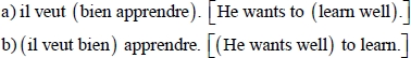
In group [4.19], in case (a) the adverb bien (well) depends on the verb apprendre (learn), whereas in case (b) this same adverb depends on the semi-auxiliary veut (wants) with which it also forms a construction of collocation type.
Obviously, syntactic ambiguity directly affects the semantic interpretation of a sentence. In fact, sometimes, multiple analyses that allow the syntax are all semantically interpretable as in the sentences [4.19] and [4.17]; and sometimes there is only a subset of these analyses that is semantically interpretable as in the sentence [4.20]:
We note in the group [4.20] that only structure (a) where the adjective expired qualifies the noun drug can receive a semantic interpretation, whereas (b) where the adjective expired qualifies the noun atherosclerosis does not have a particular meaning. With this example, we return to the concept of grammaticality which was discussed at the beginning of this section.
4.1.6. Syntactic specificities of spontaneous oral language
In the field of speech, quite a considerable number of studies has focused on phonetic and phonological aspects. However, syntax, which is a central discipline in linguistics, is the only one to remain subject to the reign of the scripturocentrism as highlighted in [KER 96]. In fact, syntactic studies have focused primarily on the written word while neglecting the oral dimension, which was considered as an impoverished and sometimes deviant form of writing. The lack of linguistic resources due to the difficulties of collecting and transcribing spoken dialogues (see [BLA 87] for a general review of these issues), as well as the relatively limited importance of the syntactic processing of the spoken language before the 1990s are some other reasons for this delay.
4.1.6.1. Topology in spoken language
Spoken language does not seem to obey the same standard as the written text regarding word order. For example, the utterances of Table 4.3 are perfectly possible in a spoken conversation or in a pseudo-writing used in discussion forums on the Internet, while they are not acceptable in a standard written text:
Table 4.3. A few examples of variation of the word order at the oral framework
Example |
Structure |
Order of elements |
My notebook I forgot it at home |
Anteposition of an NP |
OSV |
At 200 meters you will find a pharmacy |
Anteposition of an PP |
OSVO |
Me my father I love him very much |
Double marking |
SOSVO |
The question that arises is to know what is the importance of these cases in terms of frequency in the spoken conversations and then to know whether this frequency depends on the syntactic context (i.e. is it more important in a syntactic context C1 than in another syntactic context C2?). [ANT 01] have tried to answer these questions in their study which is based on three corpora of spoken French1. Thus, these researchers have shown that in ordinary situations the finalized language respects the privileged sequencing.
4.1.6.2. Agreement in gender and number
According to the constructions, agreement is often respected in the spoken language, but not always. For example, non-respect of the agreement between the noun and/or its adjectives is very rare, while non-agreement in gender between the attribute and the word to which it relates is very frequent [4.21] [SAU 72]:

4.1.6.3. Extragrammaticalities of the oral language
Extragrammaticalities, unexpected structural elements, spontaneities and disfluencies are among other terms that have been proposed in the literature to designate the spontaneous phenomena of the spoken language such as hesitation, repetition, self-correction, etc. [LIC 94, SHR 94, HEE 97, COR 99, MCK 98]. Each of these terms has its motivation. The term “extragrammaticality” which has been adopted by [CAR 83] seems to be the most appropriate, because it is sufficiently general and specific to cover the different spontaneous phenomena of the spoken language which do not depend directly on the syntax of the language. Three key phenomena are distinguished within extragrammaticalities: repetitions, self-corrections and false starts.
Repetition is the repetition of a word or a series of words. It is defined on purely morphological criteria. Consequently, the formulation and the paraphrase of a utterance or a segment (where we repeat two segments that have the same meaning) are not considered as repetitions: it would be a Paris Delhi flight rather than a flight a domestic flight.
Repetition is not always a redundancy. It can also have a communicative function. For example, when a speaker is not sure if his message (or a part of his message) will be perceived clearly by its audience because of a poor articulation, a noise in the channel, etc., he repeats it. In addition, repetition is a quite common pragmatic means to mark an affirmation or an insistence as in the utterance [4.22]:
In the utterance 4.22, the repetition of the word yes has an affirmative function.
Self-correction is to replace a word or a series of words with others in order to modify or correct the meaning of the utterance. Self-correction is not completely random and often focuses on a segment that can have one or several phrases [COR 99]. That is why it is frequently accompanied by a partial repetition of the corrected segment. Let us look at the utterance [4.23]:
In this utterance, self-correction is performed by repeating the segment I have and by replacing the word a with the word the. We note that the two words have the same morphological category (definite article) and the same syntactic function (determiner).
A false start is to abandon what has been said and starting over with another utterance. Syntactically, this is manifested with the succession of an incomplete (or an incorrectly formed) segment and with a complete segment. Let us look at the utterance [4.24]:
Unlike self-correction, there is no analogy between the replaced segment and the rest of the utterance. Thus, we can notice in the example [4.24] that the abandoned segment it is at has almost no relationship with this is taken…. This form of extragrammaticality is the most difficult to process given that the detection criteria (essentially the incompleteness of a segment) are very vague and can lead to many problems both of overgeneration and of undergeneration.
4.2. Elements of formal syntax
4.2.1. Syntax trees and rewrite rules
After reviewing the different constituents of a sentence and the subtleties of the relationships that may exist between these constituents, we will now address the question of the analysis of the sentence by assembling the pieces of the puzzle. To do this, we will begin with phrases and end with complex sentences.
The idea to use rules to describe the syntax of a particular language goes back to the beginning of the past century. It was formalized in the 1950s, particularly with [CHO 56, BAC 59].
A syntax tree is a non-oriented (there is not a predetermined direction to traverse the tree) and acyclic (we cannot traverse the tree and then return to the starting point) graph consisting of nodes connected by arcs. A node represents a constituent or a morphological or syntactic category connected by an arc with the dominant node. Each constituent must be directly dominated by the corresponding category. Inspired by family relationships, the dominant node is called “parent node” and the dominated node is called “child node”. Similarly, the highest node of a tree (the one that dominates all other nodes) is called the “root node” of this tree, whereas the lowest nodes in the hierarchy and which, therefore, do not dominate other nodes are called “leaf nodes”. In syntax trees, each word is dominated by its morphological category and phrases by their syntactic categories. Logically, the S (Sentence) is the root node of these trees and the words of the analyzed sentence are the leaf nodes.
Let us begin with the noun phrases. As we have seen, a noun phrase can consist of a proper noun only in a common noun surrounded by a wide range of varied satellite words. Let us look at the phrases in Table 4.4.
Table 4.4. Examples of noun phrases and their morphological sequences
Noun phrase |
Sequence of categories |
John |
NP |
My small red car |
Det Adj N Adj |
The house of the family |
Det N prep Det N |
As we can see in Table 4.4, each noun phrase is provided with the sequence of morphological categories of which it is composed. This sequence provides quite important information in order to understand the syntactic structure of these phrases, but it is, however, not sufficient because it omits the dependency relationships between these categories. To fill this lack of information, syntax trees can shed light on both the order of constituents and their hierarchy. Let us examine the syntax trees of the phrases provided in Figure 4.6.

Figure 4.6. Syntax trees of some noun phrases
As we note in Figure 4.6, all the trees have an NP as a root node (the highest node) since they all correspond to noun phrases. Tree (a) is the simplest one since it is a proper noun which is capable of achieving a noun phrase without another constituent. In tree (b), the kernel of the phrase, the noun car, is qualified by an anteposed adjective small and by a postponed adjective red. Tree (c) shows how a prepositional phrase acts as a genitive construction. This prepositional phrase consists in turn of a preposition and a noun phrase.
A rewrite rule is an equation between symbols of two types: terminal and non-terminal symbols. Terminal symbols are symbols that cannot be replaced by other symbols and which correspond to words or morphemes of the language in question. Non-terminal symbols are symbols that can be replaced by terminal symbols or other non-terminal symbols. In grammar, they correspond to morphological categories such as noun, verb and adjective or to syntactic categories such as NP, VP, PP, etc.
The transformation of the syntax trees shown in Figure 4.6 in rewrite rules provides the grammar in Figure 4.7.

Figure 4.7. Grammar for the structures as shown in Figure 4.6
Let us look at the noun phrase of the Figure 4.8. It is a noun phrase which includes an adverb and an adjective. What is specific in the phrase is that the adverb does not modify the noun but rather the adjective which in turn qualifies the noun. To understand this dependency relationship, the creation of an adjective phrase seems to be necessary.

Figure 4.8. Syntax trees and rewrite rules of an adjective phrase
One of the specificities of natural languages is the production capacity of an infinite number of sentences. Among the sources of this generativity is the ability to emphatically repeat the same element especially in the spoken language. Let us look at the sentence [4.25], where we can repeat the adjective an indefinite number of times:
This poses a problem because we have to repeat the same rule each time with an increase in the number of symbols (see grammar in Figure 4.9).

Figure 4.9. Grammar for the structures presented in Figure 4.8
An elegant and practical solution to this problem is to use recursive rules that contain the same non-terminal symbol, both in its left and right hand sides (grammar in Figure 4.10).

Figure 4.10. Grammar for the noun phrase with a recursion
According to the first rule of the mini grammar in Figure 4.10, a noun phrase consists of a determiner, a noun and an adjective phrase. According to our second rule, an adjective phrase consists of an indefinite number of adjectives: it adds an adjective and is called the rule of the adjective phrase. According to the third rule, the adjective phrase can consist of a single adjective and has the function to stop the looping to infinity of the second rule.
The adverbial phrase has for a kernel an adverb which can be modified by another adverb as in [4.26]:
Note that in order to avoid circularity in the analysis, we must distinguish the adverbs of degree (very, little, too, etc.) from other adverbs in the rewrite rules. This provides the rules of the form: AdvP → AdvDeg Adv.
The verb phrase is, as we have seen, the kernel of the sentence because it is the bridge that connects the subject with potential complements. Let us look at the sentences [4.27] with different complements:

These three sentences are analyzed with the syntax tree of the Figure 4.11.

Figure 4.11. Examples of VP with different complement types
Complex sentences is another type of syntactic phenomena which deserves to be examined in the framework of syntactic grammar. What is significant at this level is to be able to represent the dependencies of the clauses within the sentence.
Completives consist of adding a subordinate which acts as a complement in relation to the verb of the main clause. Thus, the overall structure of the sentence remains the same regardless of the type of the complement. The question is: how should this phrasal complement be represented? To answer this question, we can imagine that the complex sentence has a phrase of a particular type (SPh (Sentence Phrase)) which begins with a complementizer (comp) followed by the sentence. Figure 4.12 shows a parallel between a phrasal complement and a pronominal complement (ordinary NP).

Figure 4.12. Analysis of two types of sentences with two types of complements
The processing of relatives is similar to the processing of cleft sentences to the extent that we consider the subordinates as phrasal complements. Naturally, in the case of relative subordinates, the attachment is performed at the noun phrase as in Figure 4.13.
Coordinated sentences consist of two or several clauses (simple sentences) connected with a coordinating conjunction. The analysis of this type of structures is quite simple since it implies a symmetry of the coordinated constituents dominated by an element that has the same category as the coordinated elements. This rule applies both at the level of constituents and at the level of the entire sentence (see Figure 4.14).

Figure 4.13. Example of analysis of two relative sentences

Figure 4.14. Examples of the coordination of two phrases and two sentences
We should also note that syntax trees are a very good way of highlighting the syntactical ambiguity which is manifested by the allocation of at least two valid syntax trees for the same syntactic unit (see Figure 4.15).

Figure 4.15. Two syntax tree for a syntactically ambiguous sentence
At the end of this section, it seems necessary to note that phrase structure grammars, despite their simplicity and efficiency, are not a perfect solution to understand all syntactic phenomena. In fact, some linguistic cases pose serious problems for the phrase structure model [4.28]:

4.2.2. Languages and formal grammars
Formal language is a set of symbol strings of finite length, constructed on the basis of a given vocabulary (alphabet) and which is sometimes constrained by rules that are specific to this language (see [WEH 97, XAV 05] for a detailed introduction). Vocabulary, which is conventionally represented by lowercase letters of the Latin alphabet, corresponds to the words of the language which are the produced strings. To describe a formal language, the simplest way is to list all the strings produced by this language. For example, L1= {a, ab, ba, b}. The problem is that formal languages often produce an infinite number of strings whose listing is impossible. This requires the use of a formulation which characterizes the strings without having to list them all.
Let us look at L2, a formal language which includes all non-null sequences of the symbol a: L2 = {a, aa, aaa, aaaa, ….}. As it is impossible to list all the words of the language, we can use an expression of the form: {ai│i ≥1} where no limit is imposed on the maximum value of i, so as to be capable of generating an infinite number of strings. For a linguistic initiation to phrase structure and formal grammars, we refer to the books by Lélia Picabia and Maurice Gross [PIC 75, GRO 12].
When we refer to formal language, it is intuitive to evoke the concept of formal grammar. In fact, a formal language can be seen as the product of a grammar that describes it. Formally, such a grammar is defined by a quadruplet: G = (VN, VT, S, S) where:
- – VN: the non-terminal vocabulary;
- – VT: this vocabulary brings together all of the terminals of the grammar, which are commonly called the words of the language;
- – P: the set of the rewrite rules of grammar (production rules);
- – S: sometimes called an axiom, it is a special element of the set VN which corresponds to well-formed sentences.
Note that the sets VN and VT are disjointed (their intersection is zero) and that their union forms the vocabulary V of the grammar. In addition, V* denotes the set of all the strings of finite length which are formed by the concatenation of elements taken from the vocabulary including the null string and V+ is equal to V* except for the fact that it does not contain the empty string: V+ = V*− {Φ}.
Rewrite rules have the following form: α→β where α ![]() V+ ( however, it contains a non-terminal element) β
V+ ( however, it contains a non-terminal element) β ![]() V *.
V *.
Conventionally, lowercase letters at the beginning of the Latin alphabet are used to represent the terminal elements a, b, c, etc. We also use lowercase letters at the end of the Latin alphabet to represent strings of terminal elements w, x, z, etc. and the uppercase letters A, E, C, etc. to represent non-terminal elements. Finally, lowercase Greek letters represent the strings of terminal and non-terminal elements α, β, γ, δ, etc.
Let us consider a formal grammar G = (VN, VT, P, S) with:

The language defined by this grammar has the following form: L (G) = a*b. This means that the strings which are acceptable by this language are formed by a sequence of zero or more occurrences of a followed by a single occurrence of b: b, ab, aab, aaab, aaaab, etc.
To generate these language strings from the grammar, we begin with the special symbol S. We apply the set of rules which have the letter “S” in their left-hand side until there are no more terminals in the input string. The process to obtain strings from a grammar is called derivation.
Thus, in our grammar, the simplest derivation is to apply the rule #2 to replace the symbol S with the terminal b: S => b. Similarly, we can derive the sentence aab by the successive application of the rule #1 twice and the rule #2 only once: S => aS => aaS => aab.
4.2.3. Hierarchy of languages (Chomsky–Schützenberger)
After having presented languages and formal grammars, we can rightfully ask the following questions. What is the expressive power of a particular grammar? In other words, can a grammar G1 describe all the languages produced by a grammar G2? Can it describe other languages? How can we decide whether two languages described by two different formalisms are formally equivalent? To answer all these questions, the American linguist Noam Chomsky and the French mathematician Marcel Paul Schützenberger have proposed a framework for classifying the formal grammars and the languages they generate according to their complexity [CHO 56, CHO 63]. As this framework is capable of characterizing all recursively enumerable languages, it is commonly referred to as the hierarchy of languages or Chomsky hierarchy. It is a typology which includes four types of grammars, each included in the higher type and numbered between 0 and 4.

Type-0 grammar, which is also called unrestricted grammar, is the most general form of the grammar because it allows us to transform an arbitrary non null number of symbols into an arbitrary number of symbols (potentially zero symbols). It refers to grammar which accepts, for example, the rules whose right-hand side is longer than their left-hand side, as the rule: A N E → a N.
Although they are the most general, these types of grammar are the least useful for linguists and computer scientists. The languages generated by a grammar of this type are called recursively enumerable languages and the tool to recognize them is the Turing machine2.
Type-1 grammar, which is also called context-sensitive grammar, are types of grammars whose rules follow the following pattern: αAβ → αγβ.
With a non-terminal symbol A and sequences of terminal or non-terminal symbols α, γ and β knowing that α and β can be empty unlike γ. Another characteristic of these grammars is that they do not accept rules whose right-hand side is longer than the left-hand side.
The typical language generated by this type of grammars is of the form: an bn cn. This language can be generated by the grammar shown in Figure 4.17.

Figure 4.17. Grammar for the language an bn cn
The grammar in Figure 4.17 allows us to generate strings such as: abc, aabbcc, aaabbbccc, etc.

Figure 4.18. Syntax tree for the strings: abc and aabbcc
As we can see in Figure 4.18, the derivation of the abc string is performed in a direct way with a single rule: S → abc, whereas the derivation of the aabbcc string requires contextual rules such as: bEc → bbcc.
Type-1 grammar has been used for syntactic and morphological analysis particularly with augmented transition networks.
Type-2 grammar, which is called context-free grammar or context free grammar (CFG) is a type of grammar in which all rules follow the pattern: A → γ. With a non-terminal symbol A and a sequence of terminal and non-terminal symbols γ. The typical language generated by Type-2 grammar is: anbn (see Figure 4.19 for an example).

Figure 4.19. The derivation of strings: ab, aabb, aaabbb
To obtain the string ab in tree [4.19a], it is sufficient to apply the first rule: S → a B and then we replace “B” with “b” with the rule B → b. In tree (b), we apply the rule: B → a B b only once, whereas in tree (c) we must apply it twice.
Thanks to its simplicity, Type-2 grammar is quite commonly used, particularly for parsing. The automaton which allows us to recognize this type is the recursive transition network (RTN). As we will see in section 4.4.2, there is a multitude of parsing algorithms of various types to perform parsing of natural languages with context-free grammar.
Several forms, which are called normal, have been proposed to simplify Type-2 grammar without reducing their generative capacities. Among these forms, those of Chomsky and those of Greibach deserve to be addressed. Note that these normal forms retain ambiguity. This means that an ambiguous sentence generated by a Type-2 G grammar is also ambiguous in languages G’ and G’’, which are the normal forms of this grammar according to Chomsky and Greibach formats, respectively. Finally, note that the equivalence between a CFG and its standardized form is low because, although both generate exactly the same language, they do not perform the analysis in the same way.
Chomsky’s normal form imposes a clear separation between the derivation of terminal elements and the derivation of non-terminal elements. Thus, a grammar is said to be in Chomsky normal form if its rules follow the three following patterns: A →B C, A → a, S → ϵ.
Where A, B and C are non-terminals other than the special symbol of the grammar S. a is a terminal and ϵ represents the empty symbol whose use is only allowed when the language generated by the grammar is considered as a well-formed string. The constraints imposed by this normal form are that all structures (syntax trees) associated with sentences generated by a grammar in Chomsky normal form are strictly binary in their non-terminal part.
If we go back to the grammar in Figure 4.20, we note that only the rule: B→ a B b violates the diagrams imposed by Chomsky’s normal form, because its right-hand side contains more than two symbols. Thus, to make our grammar compatible with Chomsky’s normal form, we make the changes provided in Figure 4.20.

Figure 4.20. Example of a grammar in Chomsky normal form with examples of syntax trees
Note that in linguistic grammars, to avoid the three-branches rules as the one provided in Figure 4.21: NP → Det N PP, some assume the existence of a unit equivalent to a simple phrase that is called group: noun, verb, adjective, etc. (see Figure 4.21).

Figure 4.21. Syntax tree of an NP in Chomsky normal form
Grammar is said to be in Greibach normal form if all of its rules follow the two following patterns [GRE 65]: A→a and A → aB1 B2. . . Bn,
Let us consider the grammar in Figure 4.22 for an example of the grammar in Greibach normal form.
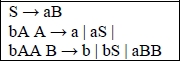
Figure 4.22. Example of grammar in Greibach normal form
It should be noted that there are algorithms to convert any Type-2 grammar in a grammar in Chomsky or Greibach normal form. We should also note that beyond their theoretical interest, some parsing algorithms require standardized grammar.
Type-3 grammar, which is sometimes called regular grammar, is a type of grammar whose rules follow the two following patterns: A → a and A → a B.
Where A and B are non-terminal symbols, whereas a is a terminal symbol. This is a typical G grammar of regular languages which generates the language: L (G) = anbm with n, m > 0 (see Figure 4.23).

Figure 4.23. Regular grammar that generates the language anbm
Finally, we should mention that it is formally proved that the languages generated by a regular grammar can also be generated by an finite-state automaton.
A particular form of regular grammar has been named “Type-4 grammar”. The rules in this grammar follow the diagram: A → a. In other words, no non-terminal symbol is allowed in this type of grammar. This grammar, which is of limited usefulness, is used to represent the lexicon of a given language.
Table 4.5 summarizes the properties of the types of grammar that we have just reviewed.
Table 4.5. Summary of formal grammars
| Type | Form of rules | Typical example | Equivalent model |
| 0 | α → β (no limits) | Any calculable function | Turing machine |
| 1 | αAβ → αγβ | anbncn | Augmented Transition Networks (ATN) |
| 2 | A → γ | anbn | Recursive Transition Networks (RTN) |
| 3 | A → a A → aB |
a* = an | Finite-state automata |
The presentation of the different categories of formal languages and their principal characteristics leads us to the following fundamental question: what type of grammar is able to represent all the subtleties of natural languages? To answer this question, we are going to discuss the limits of each type based on Type-3 grammar.
From a syntactic point of view, natural languages are not regular because some complex sentences have a self-embedded structure which requires Type-2 grammar for their processing (examples [4.29]):

To understand the differences between the abstract structures of complex sentences, let us look at Figure 4.24.

Figure 4.24. Types of branching in complex sentences
The syntax of natural languages is not independent of context because, in a language such as French, there is a multitude of phenomena, whose realization requires the consideration of the context. For example, we can mention the following: agreement, unbounded dependencies and passive voice.
Agreement exists between certain words or phrases in person, number and gender. In a noun phrase, the noun, the adjective and the determiner agree in gender and number. In a verb phrase, the subject and the verb agree in person and number. To integrate the constraints of agreement in a Type-2 grammar, we must diversify the non-terminals and then create as many rules for the possible combinations. The rule S → NP VP will be declined in six different rules as in the context-free grammar shown in Figure 4.25.

Figure 4.25. Type-2 grammar modified to account for the agreement
This solution significantly reduces the generative power of grammar and makes its management very difficult in practice, because non-terminals are difficult to be read by humans. Some cases of agreement are even more complicated, as the agreement between the post-verbal attributive adjective of an infinitive and the subject noun phrase [4.30]:
Type-2 grammar does not allow us to specify the sub-categorization of a verb predicate (the required complements) or to require that the verb does not have complements. Here a possible solution is also to vary categories. These types of grammar do not allow the expression of structural generalizations such as the relationship between the passive and the active voice.
4.2.4. Feature structures and unification
The formalisms that we have just seen allow us to represent the information on the hierarchical dependencies of the constituents and their order. We have seen that with the grammar in Figure 4.25, it is quite important to take into account the relationships of agreement between these different constituents with a simple phrase structure grammar. The most current solution in the field of linguistics to solve this problem is to enrich the linguistic units with feature structures (FS), which contain information of different natures (morphological, syntactic and semantic) and to express the possible correlations among them. They also allow us to refine the constraints at the lexicon level and, thus, to simplify the rules of grammar. For more information on feature structures and unification, we refer to [SHI 86, CHO 91, WEH 97, SAG 03, FRA 12].
As we have seen in the sphere of speech, the first use of features in modern linguistics was proposed in the field of phonology, particularly with studies by Roman Jacobson, Noam Chomsky and Morris Halle. Since the 1980s, FSs have been adopted in the field of syntax, particularly in the framework of formalisms based on unification. It is a family of linguistic formalisms that allows us to specify lexical and syntactic information. The main innovation of these formalisms lies on two points: the use of features for encoding of information and the unification operation for the construction of higher constituents than the word level.
The unification operation is applied on features in order to test, compare or combine the information they contain. The origin of the unification concept is double: on the one hand, it comes from the studies on the logic programming language “Prolog” [COL 78, CLO 81] and on the other hand, it is the result of studies in theoretical and computational linguistics on the functional unification grammar (FUG) [KAY 83], the lexical functional grammar (LFG) [BRE 82, KAP 83] and the generalized phrase structure grammar (GPSG) [GAZ 85].
We distinguish two types of feature structures: atomic feature structures in which all features have a simple value and complex feature structures (CFS) where features can have other feature structures as a value. Below is the structural feature of the noun “house” and of the verb “love” which are shown in Figure 4.26. For example, the verb (FS b) has two features: an atomic feature VerbType and a complex feature Agreement.

Figure 4.26. Feature structures of the noun “house” and of the verb “love”
Beyond the words, all other levels, such as phrases, clauses and sentences, can be enriched by CFSs. To clarify the enrichment of supralexical units with features, let us take a simple sentence such as [4.31]:
As there is no consensus as to the necessary features for the analysis of a sentence, the linguistic theories which adopt the features as a mode of expression of linguistic properties differ on this point. Thus, we can adopt the following features to analyze the sentence [4.31]:
- – category: specifies the grammatical category of the sentence: S;
- – head: corresponds to the head of the sentence which is the verb and specifies the features: tense, voice, and number;
- – subject: noun phrase which is an argument of the verb;
- – object: noun phrase which is an argument of the verb.
This provides the CFS presented in Figure 4.27.

Figure 4.27. CFS of a simple sentence
A variant of the feature structures was proposed by Aït-Kaci [AIT 84] where each structural feature has a type which limits the features that can be included, as well as the values that the atomic features can have. This concept is comparable to the types in the framework of the object-oriented programming. For example, the complex feature subject can understand the category and agreement features and the atomic feature Nb. can have the values: sing and plur.
We should also note that CFSs can take the form of feature graphs, such as the examples of the feature structures presented in Figure 4.28.
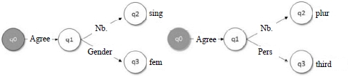
Figure 4.28. Feature graphs for the agreement feature for the words “house” and “love”
As we see in Figure 4.28, feature graphs are oriented, as we cannot navigate in the direction of the arrow (or arc). As these graphs are a data structure whose mathematical properties are well-known, this allows us to improve our understanding of CFS properties. Such a graph can be seen as a quadruplet: {Q, q’, δ, θ}. Let us look at the graph (a) in Figure 4.28 as an example, to make our explanation more concrete.
- – Q is a finite set of nodes: Q = {q0, q1, q2, q3};
- – q’ ϵ Q is the initial state of the graph q’ = q0. As we can note, in Figure 4.28, the initial state of this graph is colored to differentiate it from other states;
- – δ represents a partial function in the graph such as: δ(q0, Agreement)= q1, δ(q1, Nb.)= q2, δ(q1, Gender)= q3;
- – θ represents a leaf that corresponds to a feature. Thus: θ(q2)=sing, θ(q3)=fem.
The representation of the features in the form of a graph leads us to the path concept which is intimately associated with this. A path is a sequence of features used to specify a particular component of a structural feature. The paths that interest us are those that connect the initial element and a leaf. If we accept that a path is part of our CFS: π ϵ CFS, we can say that our function δ(q, π) provides the value of path π from the node q. Now, if two different paths begin with the initial state of the graph and ultimately lead to the same node, we then say that there is a reentrancy relationship between these two paths. Formally, we can express this as: δ(q0, π) = δ(q0, π’) and π≠π’. By extension, a structural feature is called reentrant if it contains two features that share a common value. It is appropriate to distinguish the reentrancy of cases where two different paths lead to two different features which occasionally have the same value. In this kind of case, we refer to paths of similar values. Let us consider the examples of CFSs in Figure 4.29 to clarify this distinction.

Figure 4.29. Example of structures of shared value and of a reentrant structure
As we can see in Figure 4.29, structures of similar values consist of an occasional resemblance between the values of different features (q3 and q4). This means that it is not a constraint imposed by grammar but a simple coincidence. A current example is when two noun phrases, subject and object direct, share the same features of agreement in gender and number. By contrast, the reentrant features are the shared product of two different paths of the same feature (q4) as in the constraints on the agreement between two different constituents as the subject noun phrase and the verb phrase.
In matrix form, reentrant features are marked with specific indices. Thus, the symbol ![]() in Figure 4.30 means that the features f and g must have the same value.
in Figure 4.30 means that the features f and g must have the same value.

Figure 4.30. Example of structures of shared value and of a reentrant structure
If we approach the issue of the comparison of two feature structures, a key question arises: are there any CFSs which are more generic than others? To answer this question, the concepts of subsumption and extension have been proposed.
Subsumption is a partial order relationship that we can define on feature structures and which focuses both on the compatibility and the relative specificity of the information they contain. It is noted with the help of the symbol: ⊆. Let us look at the two feature structures FS and FS’. We say that FS is a subsumption of FS’ if all information contained in FS is also present in FS’.
In Figure 4.31, we have three CFSs that maintain the following subsumption relationships: a ⊆ b and a ⊆ c and b ⊆ c. In other words, as the CFS a is the least specific and consequently more abstract, it subsumes the structures b and c which are more generic. Obviously, the subsumption between these structures would not exist without the compatibility between these three structures. If we go back to Figure 4.26, the feature of agreement of the structure (a) does not subsume the feature of agreement of (b) and vice versa, because of the incompatibility between the two features: the feature gender in (a) and the feature pers in (b).

Figure 4.31. Examples of feature structures with subsumption relationships
Extension is the inverse relationship of subsumption. It can be defined in the following manner: let us consider two structures FS and FS’. We can say that FS’ is an extension of FS, if and only if: all atomic features of FS’ are present in FS with the same values, and if for all non-atomic features ti, in FS’, there is an atomic feature ti’ in FS such that the value of ti’ is an extension of the value of the feature ti.
Naturally, all feature structures are not in a relationship of extension or subsumption. In fact, some CFSs can contain different but compatible information, such as the relationship between the object and the subject in matrix (c) as shown in the Figure 4.25. In addition, the structures “subject” and “head” are both different and incompatible.
We have seen that the syntactic analysis process consists of combining the representations of syntactic units to achieve a representation of the structure of the sentence. We have also seen examples of syntactic operations which allow us to combine words and phrases, etc. The question which arises at this stage is: how can we combine the representations of constituents enriched with features? The answer to this question is to use the unification operation. It is an operation which determines, from a set of compatible structures, a structure that contains all the information present in each of the members of the set and nothing else. The unification of the two feature structures FS1 and FS2 has, as a result, the smallest structure FS3 which is an extension both of FS and FS’. If such a structure does not exist, then the unification is indefinite. Symbolized by the union operator U, unification can also be reformulated:

Note that the unification operation is both commutative and associative:

As we can see in Figure 4.32, unification can be performed in quite varied configurations. In case (a), it is clear that the unification of a structural feature with itself is possible. Case (b) shows how we can unify the two different structures to obtain a richer structure. Case (c) shows that logically the unification of two incompatible feature structures is impossible because it leads to an inconsistency. In case (d), we see that the null structure acts as a neutral element and unifies with all structures without modifying them. Case (e) shows how we can perform unification with reentrant features. Finally, in case (f), we see a unification operation of more complex linguistic structures.
It should be noted that there are several generic tools that provide implementations of the unification process and which are available to the community. Among the best-known we can mention: PATRII, Prolog, and NLTK.
The logic programming language “Prolog”, as we have seen, is the tool which inspired the first studies and is still valid. In fact, the unification of terms which are provided natively in Prolog significantly reduces the application development time.
PATRII is another tool available to the community in the field of unification. Originally proposed in SRI International by Stuart Shieber, PATRII is both a formalism and a programming environment written in Prolog [SHI 87]. It is possible to use PATRII to implement a limited variety of formalisms. It is based on Type-2 grammars with which FS are associated.

Figure 4.32. Examples of unifications
4.2.5. Definite clause grammar
Definite clause grammar (DCG) is a logical representation of linguistic grammars. The first form of this grammar, which was called “metamorphosis grammar”, was introduced in 1978 at the University of Marseille following Alain Colmerauer’s studies, of which the first application was on automatic translation. Afterward, David Warren and Fernando Pereira of the University of Edinburgh proposed a particular case of metamorphosis grammars which were named DCG [PER 80]. DCGs were created to develop and test grammars on the computer, particularly with the logic programming language “Prolog” and more recently with the language “Mercury”. From a functional point of view, DCGs allow us to analyze and generate string lists. Let us look at the DCG in Figure 4.33.

Figure 4.33. DCG Grammar
The first note that we can make in respect of the grammar in Figure 4.31 is that its format is very close to the format of the ordinary Type-2 grammars, apart from a few small details. For example, non-terminals do not begin with a capital letter. As the latter is the indication of a variable according to the syntax of Prolog, terminals are provided in square brackets which are used in Prolog to designate lists. We also note that DCG allows the writing of recursive rules (the p symbol exists in the left and the right-hand side of the rule).
It is also necessary to add that DCGs can be extended to enrich the structures with features (see grammar in Figure 4.34).

Figure 4.34. DCG enriched with FS
Several extensions have been proposed to improve DCGs including XGs by Pereira [PER 81], the definite clause translation grammars (DCTGs) by [ABR 84] and the multi-modal definite clause grammars (MM-DCGs) by [SHI 95].
4.3. Syntactic formalisms
Given the interest in syntax, a considerable number of theories in this field have been introduced. Different reasons are behind this diversity, including the disagreement on the main units of analysis (morpheme, word or phrase), the necessary knowledge to describe these units, as well as the dependency relationships between them.
In this section, we retained three formalisms, including two that are based on unification: X-bar, HPSG and LTAG.
4.3.1. X-bar
Before introducing the X-bar theory, let us begin with a critical assessment of the phrase structure model presented in section 4.2.1. Let us look at the sentences [4.32] and the rewrite rule and the syntax tree of the sentence [4.32a] shown in Figure 4.35:


Figure 4.35. Rewrite rule and syntax tree of a complex noun phrase
The sentence [4.32a] mentions a pharmacist in the city of Aleppo who has a blue shirt and the sentence [4.32b] mentions a reportage of Istanbul about the Mediterranean. Intuitively, we have the impression that the two prepositional phrases in the two cases do not have the same importance. To demonstrate this, it is sufficient to perform a permutation between the two phrases in each of the sentences. This provides the sentences [4.32c] and [4.32d] which are not semantically equivalent, initial sentences ([4.32a] and [4.32b]) whose grammaticality is questionable. Thus, we can conclude that the two prepositional phrases do not have the same status. However, the plain phrase structure analysis proposed in Figure 4.35 assigns equal weight to them. Consequently, a revision of our model seems necessary in order to account for these syntactic subtleties.
Moreover, in the framework of a universal approach to the modeling of the language, we observe that the rules that we have proposed up to now are specific to the grammars of European languages such as English or French and do not necessarily apply to other languages such as Arabic, Pashto or Portuguese.
These considerations, among others, led to the proposal in 1970 of a modified model of the generative and transformational grammar which was named X-bar theory. Initiated by Noam Chomsky, this theory has been developed afterwards by Ray Jackendoff [CHO 70, JAC 77]. It allows us to impose restrictions on the class of possible grammatical categories while allowing a parallel of these latter elements thanks to metarules (generalization of several rules). It is also a strong hypothesis on the structure of constituents across languages. It rests on two strong hypotheses:
- – all phrases, regardless of their categorical nature, have the same structure;
- – this structure is the same for all languages, regardless of the word order.
The term X-bar is explained as follows. The letter X corresponds to a variable in the general diagram of the structure in constituents, which applies to all syntactic categories (N, V, A, S, Adv., etc.). The term bar refers to the notation adopted by this formalism to differentiate the fundamental levels in the analysis. They are noted with one or two bars above the categorical symbol of the head. Usually, for typographical reasons, we replace the notation bar with a prime notation. N”, V”, A” and S” are thus notational variants respectively of NP, VP, ITS, PP. The notation that we have adopted and the alternatives in the literature are presented in Table 4.6.
Table 4.6. Adopted notation and variants in the literature
| Level | Our notation | Alternatives |
| Phrase level | NP | N”, N", |
| Intermediate level | N’ | |
| Head/Word level | N | N0 |
In the framework of the X-bar theory, a phrase is defined as the maximum projection of a head. The head of a phrase is a unique element of zero rank, word or morpheme, which is of the same category as the phrase as in the grammar of the Figure 4.36.

Figure 4.36. Examples of phrases with their heads
This leads us to a generalized and unique form for all rules: SX → X SY, where X and Y are variables. Furthermore, according to the X-bar theory, a phrase accepts only three analysis levels:
- – level 0 (X) = head;
- – level 1 (X) = head + complement(s);
- – level 2 (X) = specifier + [head + complement(s)].
The specifier is usually an element of zero rank, but sometimes a phrase can have this role: NP (spec(my beautiful) N0 (flowers)). The specifier is a categorical property of the head word. For example, the determiner is a property of the category of nouns. Similarly, the complement is a lexical property of the head word: taking two object complements by the verb give is a lexical property of this specific verb, not a categorical property of the verb, in general. Let us examine the diagrams of the general structures of the phrases provided in Figure 4.37.

Figure 4.37. Diagrams of the two basic rules
In the two diagrams shown in Figure 4.37, we have the symbols X, Y and Z which represent the categories, Spec (X) which corresponds to a specifier of and Comp(X) for complement of. The categories specifier and complement designate the types of constituents. Thus, we have:
- – Spec N = D (Det);
- – Spec V = Vaux;
- – Spec A = DEG (degree);
- – Comp X’ = N”.
The hierarchical structure of the two syntactic relationships specifier and complement induces a constraint on the variation of order within the phrases. The X-bar theory predicts that the complement can be located to the left or to the right of the head and that the determiner is placed to the left of the “head+complement” group, or to the right of this group.
If we go back to our starting noun phrase a pharmacist from Aleppo with the blue shirt or even a variant of this phrase with an antepozed adjective to the noun phrase such as good, we obtain the analyses provided in Figure 4.38.

Figure 4.38. Examples of noun phrases
As we observe, the analyses proposed in Figure 4.38 take into account the functional difference between the two prepositional phrases. Similarly, the adjective responsible with respect to the head is processed as a specifier of the head of the phrase.
Although they appear to be acceptable, some researchers have doubted the adaptation of the analyses proposed in Figure 4.39 with respect to the principles of the X-bar theory. In fact, one of the principles, which form the basis of this theory, is to consider that all constituents, other than the head, must themselves be phrases. It is rather motivated by reasons related to the elegance of the theory than by linguistic principles. In the case of a noun phrase, this means that the only constituent that is not phrasal is the noun. However, in the proposed analysis, the determiner is analyzed similarly to the head. To resolve this problem, some have proposed an original approach which is to consider that NP depends in reality upon a determiner phrase whose head is the determiner [ABN 87]. The diagram of an NP according to this approach is provided in Figure 4.39.

Figure 4.39. Diagram and example of a determiner phrase according to [ABN 87]
The processing of the verb phrase follows the standard diagram as can be seen in Figure 4.40.
After having shown how we analyze noun, verb and prepositional phrases in the framework of the X-bar theory, it is time to proceed with the analysis of an entire sentence. We have seen that it is generally easy to adapt the conventional analyses of constituents in the framework of the X-bar theory, but this is less obvious in terms of the sentence itself. Consider the conventional rewrite rule for the sentence: S → NP VP. The question that arises is to determine if the root of the sentence S is a projection of V (the head of VP) or a projection of N (the head of the subject NP). Two syntactic phenomena deserve to be examined prior to decide. Firstly, we must report the phenomenon of agreement between the subject NP and the VP in our sentence analysis. To do this, it would be useful to postulate the existence of a node between the subject NP and the VP, which would establish the link of agreement between these two phrases. Secondly, we can observe differences in the behavior of infinitive verbs and conjugated verbs. The two differ in the place they occupy with respect to the negation markers, certain adverbs and quantifiers. These differences confirm the special relationship which connects the conjugate verb with the subject noun phrase since it does not allow an interruption by these particular words. Invariably, the infinitive verb has no relationship of agreement with the subject (see [ROB 02] for some examples in French).

Figure 4.40. Example of the processing of a verb phrase with the X-bar theory
To account for the relationship between the subject NP and the VP, we can use an intermediate node between these two constituents. The role of this node is to convey the necessary information to the agreement of the verb AGG with the subject, as well as to provide the tense T. This node is called Inflectional Phrase (IP). We can now postulate that the sentence is a maximum projection of IP and that its head is, therefore, IP (see Figure 4.41).

Figure 4.41. Diagram and example of analysis of entire sentences
The analysis of complex sentences is similar, in principle, to the analysis that we have already seen in the previous section. We assume the existence of a phrasal complement (PC) (see Figure 4.2).

Figure 4.42. Analysis of a completive subordinate
Despite its elegance and its scientific interest, the X-bar theory has several limitations. Among them, we should mention the problem of infinitives and proper nouns, where it is difficult to identify the head.
The step that has followed the X-bar theory in the generative syntax was the proposal of the government and binding (GB) theory by Noam Chomsky at the beginning of the 1980s [CHO 81]. We refer to [POL 98, ROB 02, CAR 06, DEN 13] for an introduction to this formalism, of which we will present only the general features.
To account for the different aspects of the language, GB is designed in a modular fashion involving a set of principles of which the most important are:
- – government principle: this principle describes the phenomena of reaction. It addresses all conditions and constraints between the governors and those being governed;
- – instantiation criteria of thematic roles: each lexical head associates the syntactic roles with their arguments (theta roles). Each argument of the sentence must receive a role and each and every role must be distributed. To receive a case, there must be a lexical or governed entity;
- – binding principle: this principle describes the phenomena of co-referential anaphora.
In spite of its high complexity, GB formalism has been the subject of several operations in different application contexts [SHA 93, WEH 97, BOU 98]. GB formalism has, in turn, been the subject of amendments in the framework of Chomsky’s minimalist program [CHO 95].
Finally, it is probably necessary to add that some concepts of the X-bar theory have also found their place in the theories related to generative grammar, including the HPSG formalism, to which we will devote the next section.
4.3.2. Head-driven phrase structure grammar
4.3.2.1. Fundamental principles
Head-driven phrase structure grammar (HPSG) was originally proposed to combine the different levels of linguistic knowledge: phonetic, syntactic and semantic. This formalism is presented as an alternative to the transformational model [POL 87, POL 96, POL 97]. Although it is considered as a generative approach to syntax, HPSG is inspired by several formalisms which come from several theoretical currents, including the generalized phrase structure grammar (GPSG), the lexical functional grammar (LFG) and the categorial grammar (CG). In addition, there are notable similarities between HPSG and construction grammar (CG) which can be noted. In fact, although CG focuses on essentially cognitive postulates, it has several points in common with HPSG, particularly with regard to the flexibility in the processing unit, as well as the representation of linguistic knowledge within these units [FIL 88] (see [GOL 03] and [YAN 03]). The legacy of these unification grammars, heirs themselves of several studies in artificial intelligence and cognitive sciences on the representation and the processing of knowledge, makes HPSG particularly suitable for IT implementations, which explains its popularity in the NLP community.
The processing architecture in the HPSG formalism is based on the single analysis level and does not therefore assume levels distributed as in the LFG formalism with the double structures: functional structure and structure of constituents. This is the same concerning the transformational model which assumes the existence of a deep structure and of a surface structure, or even as the GB model that attempts to explain the syntactic phenomena with the movement mechanism.
From a linguistic point of view, HPSG is composed of the following elements:
- – a lexicon: which groups the basic words which are, in turn, complex objects;
- – lexical rules: for derivative words;
- – immediate dominance patterns: for structures of constituents;
- – rules of linear precedence: which allow us to specify word order;
- – a set of grammatical principles: which allow us to express generalizations about linguistic objects.
Since the complete presentation of a formalism as rich as the HPSG is difficult to achieve in a small section such as this, we refer the reader to the articles by [BLA 95, DES 03], as well as to Anne Abeillé’s book [ABE 93] (in particular, the chapters on the GPSG and HPSG formalisms). We also refer to Ivan Sag’s book and his collaborators [SAG 03] which constituted the primary source of information for this section.
4.3.2.2. Feature structures
FSs have a main role in the framework of HPSG formalism. More specifically, it refers to typed features, which means that to be well-formed, an FS must contain all the features required by its type and that all these features must be well instantiated. The types are organized in a generic hierarchy whose highest element is a sign. Words, phrases, sentences and speech are represented as signs as recommended in Saussurean tradition. Each sign has phonetic, syntactic and semantic characteristics which are grouped in an FS, whose general diagram is provided in Figure 4.43. The use of types in the development of the lexicon makes the latter more compact, thus facilitating its management and processing, and assuring its consistency. On the processing plan, types allow us to control the unification operation and consequently to avoid its failure.

Figure 4.43. Diagram of a typed FS in HPSG
The sign feature has the function to indicate the status of the constituent at the head of which it is located. The PHON feature is used to list the words of the constituent. Exceptionally, it allows us to indicate the phonological properties of the constituent. The SYNSEM feature represents the syntactic and semantic features which describe the constituent. Sometimes, we prefer to have two separate features: SYN and SEM. The SYN feature provides the grammatical category of the node, its inflectional properties, as well as the nodes with which this element must be combined, whereas The SEM feature specifies the manner in which the sentence will be interpreted (mode of the sentence, participants, situation, etc.). LOC and NON-LOC features concern respectively the intrinsic/extrinsic aspects of the constituent which focus on its internal structure and its relationships with the objects that are located in its syntactic context. Most of the syntactic constructions are processed locally except for particular constructions, such as movement, which require non-local processing (see Table 4.7).
Table 4.7. Types in HPSG formalism [POL 97]
Type |
Subtype |
sign |
word, phrase |
phrase |
headed phrase, headless phrase |
list (σ) |
nelist(σ) (nonempty list), elist (empty list) < > |
set (σ) |
neset(σ) (nonempty set), eset (empty set) |
content |
relationship, indexed-obj |
relationship |
gives-rel, walks-rel,... |
Head |
nomin, verb, adj, prep, ... |
Case |
noun, accus |
Index |
Per, Noun, Gender |
Finally, DTRS node concerns child nodes and leads to two features: NON-HEAD-DTRS and HEAD-DTRS. To clarify the diagram provided in Figure 4.43, let us take the example of the FS in Figure 4.44.

Figure 4.44. Simplified lexical entry of “house”
According to the FS provided in Figure 4.35, the word house is of the noun category and it has the features of agreement: 3rd person and singular. It also says that this word must have a specifier (determiner), which has exactly the same features of agreement as the head, due to the use of a reentrant feature and an optional complement, placed between two parentheses, of a prepositional phrase type. Note that, in view of the wealth of FS in HPSG, many abbreviated forms or notational equivalents exist in the literature (see Figure 4.45 for a presentation).

Figure 4.45. Some abbreviations of FS in HPSG
The S-ARG or ARG-S feature concerns the argument structure which focuses on the relationships of binding of argument predicates. For example, verbs such as see, love and write can have the following argument structure: <see, [S-ARG < NP, NP>]>.
The FS of our lexical entry can be further enriched particularly with the addition of semantic features. Among them, we should mention MODE, INDEX and RESTR features. The MODE feature provides the semantic modes of an object and can have the values: question, proposal, reference, direction or none. The INDEX feature can take a theoretically unlimited number of values which correspond to the entities or the situation to which a constituent (or an entire sentence) can refer. Finally, the RESTR feature, whose value is a list of conditions, concerns conditions on the entities or the situation described by the INDEX feature, as well as the relationships that there may exist between them. If we take the word love, we have the following restrictions: the noun of the RELN relationship is love and this relationship implies two actors or entities: loving and loved; and in a specific situation, SIT. Similarly, the verb give implies a donor, a receptor and an object/gift always in a specific situation s.
Let us examine the two FSs of word inputs: house and John provided in Figure 4.46. In fact, this figure provides an enriched FS with S-ARG and SEM structure features of arguments. The S-ARG feature indicates that the specifier must be concatenated by the symbol ⊕ with the complementer. Semantic features indicate that this noun is of the type reference and that it has an index k. The proper noun John, meanwhile, has a simpler FS: the values of syntactic features, specifiers, complements and modifiers are empty. On the semantics level, it has a relationship of a proper noun (NP), which applies to a named entity.

Figure 4.46. Enriched FS of the words “house” and “John”
With regard to verbs, features vary depending on the relationship of the verb with its arguments (transitive or intransitive verbs, etc.). Let us take the simplified examples shown in Figure 4.47.

Figure 4.47. Some simplified FS of verbs
The transitive verb hits takes two arguments: a subject noun phrase and an object noun phrase at the nominative case and the third person singular. The verb continues takes a verb phrase as a complement. Finally, the verb dies, being intransitive, has an empty list of complement.
A more complete example of a verb is provided in Figure 4.48.

Figure 4.48. FS of the verb “sees”
The verb sees has two arguments: a subject noun phrase to the nominative case, which has the semantic role of voyeur, and an object noun phrase in the accusative case whose semantic role is seen.
4.3.2.3. Morphological rules
Lexical rules concern the introduction of morphological rules to FS of words in order to avoid redundancies, e.g. repeating the same FSs once for the singular form and once more for the plural form is expensive both in terms of grammar writing and in terms of memory, without mentioning the elegance of grammar and cognitive issues.
A lexical rule is an FS which establishes a link between two lexical sequences. We distinguish between two types of lexical rules l-rules: the rules of inflection i-rules, and the rules of derivation d-rules. All lexical rules obey the constraints described by the diagram in Figure 4.49.

Figure 4.49. General diagram of l-rules
Let us begin with i-rules. As we have seen in the sphere of morphology, inflection focuses primarily on the plural and singular forms for nouns, as well as the conjugation for verbs. To obtain a plural form for a noun from the singular form, we simply have to find the corresponding form according to the morphophonological rules that we have already seen, as well as to update the structural feature (see the example in Figure 4.50).

Figure 4.50. Rule of plural
According to the rule illustrated in Figure 4.50, the plural form of a countable noun is a structure that keeps all the features of the singular structure, but with the NB feature of the agreement, which become plural. Obtaining the plural form of the noun is performed with the function of the plural noun FNPL. The other forms of inflection and derivation follow the same principle. Let us take the case of the derivation of an agent noun from the verb: dance → dancer (Figure 4.51).

Figure 4.51. Rule of derivation of an agent noun from the verb
The function F-er adds an appropriate suffix to the form of the word at the output. The input of the rule is a verbal lexeme, whose INDEX feature of semantics becomes i at the noun form, because the change involves important semantic modifications resulting from the derivation, including the value of the MODE feature. By contrast, the value of the RESTR feature remains unchanged in both forms, because the information provided in the verbal form is compatible with the noun form. The ARG-FS feature requires a complement because, in languages such as English and French, we cannot get an agent noun from an intransitive verb: give → giver, play → player, but not die → dier. Followed by a genitive construction in French, an agent noun is located in a preposition phrase before the preposition de (of) as in donneur de sang (blood donor) and joueur de football (football player).
It is probably necessary to point out that, in cases where both mechanisms of derivation and inflection are necessary, we must first apply the rule of derivation and then the rule of inflection.
4.3.2.4. Syntactic rules
Unlike formalisms such as LFG and GB, the construction of the phrase is performed by combining and satisfying the constraints expressed by words. Several rules of word combination to form larger syntactic constituents are possible. We have selected the three rules that we considered to be the most important and which correspond to the basic rules of the X-bar theory.
The Head-Complement Rule takes the head H and produces a phrase if this head is located in a sequence of arguments which are compatible with the requirements for its COMPS feature. The FS of the obtained phrase is identical to the features of the head, except for COMPS features that are saturated (realized) and therefore removed by convention. In other words, in HPSG, the head produces a phrase which is similar in a manner compatible with the X-bar principle: the phrase is a maximum projection of the head. In addition, the labels ![]() must be the same in the following phrases. This means that the elements in the right-hand side of the rule must be selected by COMPS feature (see Figure 4.52).
must be the same in the following phrases. This means that the elements in the right-hand side of the rule must be selected by COMPS feature (see Figure 4.52).

Figure 4.52. Head-Complement Rule
If we apply the rule of Figure 4.52 to a transitive verb and a noun phrase, this provides the tree of the Figure 4.53 where we have retained only the relevant features.

Figure 4.53. Head-Complement Rule applied to a transitive verb
We note in the tree structure of Figure 4.53 that the features of the head of the child node become the head features of the entire phrase. This is due to the Head Feature Principle (HFP) according to which the values of the head of any phrase are identical to the values of the head of the child node. We also note that the value of the SPR feature of the head of the child node is also transferred to the parent node. This is due to the Valence Principle (VP) which stipulates that the values of SPR and COMPS features must be identical to those of the head of the child node unless the rule specifies otherwise.
The Head-Modifier Rule allows us to obtain a phrase of a level equivalent to the X’ in the X-bar theory. The MOD feature of the modifier must have the same value as the element it modifies (see Figure 4.54). Note that the HFP principle makes this rule generic (independent of the syntactic category), just as in the X-bar theory.

Figure 4.54. Head-Modifier Rule
The Head-Specifier Rule (Figure 4.55) takes a phrase with an SPR feature whose value is non-empty and combines it with an item that satisfies this value. The result is a phrase with a head preceded by a specifier.

Figure 4.55. Head-Specifier Rule
4.3.2.5. Semantic principles
After having examined some syntactic rules for the combination of the constituents, we will now examine the semantic constraints which allow us to enrich syntactic structures with semantic properties. The two most important principles are: the Principle of Semantic Compositionality and the Semantic Inheritance Principle. The Principle of Semantic Compositionality stipulates that in any well-formed phrase, the RESTR feature of a parent node is the sum of the values of its child nodes. Similarly, the Semantic Inheritance Principle specifies that the values of MODE and INDEX features are identical to HEAD features of the child nodes. This means that in the HPSG formalism, semantics, just as syntax, is led by the head.
4.3.2.6. Example of an analysis of a simple sentence
To complete our presentation of the HPSG formalism, let us consider an example of the analysis of the following sentence: He sees the house. We will begin with the object noun phrase and to do this, we must first specify the FS of the determiner the as we have already seen the lexical entries of the noun house (Figure 4.46), as well as of the verb sees (Figure 4.48). Note that, for presentation conciseness reasons, we have seen fit to simplify the FSs.

Figure 4.56. Lexical entry of the determiner “the”
The single element that deserves a comment in the FS of the Figure 4.56 is the Bound-variable (BV) feature. In fact, the semantic framework adopted for the quantifiers is the generalized quantifier theory which models both the standard quantifiers, such as the universal and existential quantifiers, and the non-standard quantifiers, such as the most or the large majority in the framework of the set theory.
As we can see in the tree of Figure 4.57, the FS of the determiner is identical to the FS of the determiner presented in Figure 4.56 with a few notable differences. On the one hand, the FS is marked by the symbol ![]() , which allows us to insert the FS of the determiner the in the list of specifiers of the noun house allowing, according to the Head-Specifier Rule, the combination of these two words in the framework of the NP.
, which allows us to insert the FS of the determiner the in the list of specifiers of the noun house allowing, according to the Head-Specifier Rule, the combination of these two words in the framework of the NP.
Similarly, the Semantic Inheritance Principle implies that the phrase inherits the MODE and INDEX features of the head node which are respectively: ref and k. This unifies the indexes of the and house and allows the determiner to quantify the noun in the framework of the noun phrase. Moreover, according to the principle of semantic compositionality, the value of a REST node of a parent node is the sum of the values of the child nodes: ![]() .
.

Figure 4.57. Feature structures of the noun phrase: the house
We are now ready to examine the analysis of the verb phrase: sees the house (Figure 4.58).

Figure 4.58. Analysis of the verb phrase: sees the house
Several observations can be made about the Figure 4.58. The noun phrase, labeled by the symbol ![]() , whose FS is an abbreviation of the noun phrase of the Figure 4.57, is inserted in the list of the verb complements. Moreover, according to the Head-Complement Principle, the FS of the produced phrase is identical to that of the head of the complement, except for the COMPS feature whose value is empty (saturated). The value of the RESTR feature in the phrase is the concatenation of the values of the RESTR features in the child nodes:
, whose FS is an abbreviation of the noun phrase of the Figure 4.57, is inserted in the list of the verb complements. Moreover, according to the Head-Complement Principle, the FS of the produced phrase is identical to that of the head of the complement, except for the COMPS feature whose value is empty (saturated). The value of the RESTR feature in the phrase is the concatenation of the values of the RESTR features in the child nodes: ![]() and
and ![]() . According to the Valence Principle, the value of the SPR node of the root node is equal to the value of the SPR node of the head of the child node.
. According to the Valence Principle, the value of the SPR node of the root node is equal to the value of the SPR node of the head of the child node.
To analyze the entire sentence, we still have to introduce the FS of the subject pronoun, which is presented in Figure 4.59, as well as its combination with the structure of the Figure 4.60.

Figure 4.59. The FS of the pronoun “the”
To complete the analysis of the sentence, we still have to combine the structure constructed for the verb phrase (verb + complement NP) with the FS of the subject pronoun he, which provides the representation of Figure 4.60. The value of the RESTR node is the result of the concatenation of: ![]() . The value of the AGR feature in the root node is equal to the value of the subject and in accordance with the Head Feature Principle (HFP) the Head-Specifier Rule, as well as the constraint of agreement between the verb and its specifier.
. The value of the AGR feature in the root node is equal to the value of the subject and in accordance with the Head Feature Principle (HFP) the Head-Specifier Rule, as well as the constraint of agreement between the verb and its specifier.
HPSG has been applied to several languages of various families, such as Arabic, French, German, Danish, etc. The deep linguistic processing with HPSG (DELPH-IN3) initiative has allowed the development of grammars of large sizes for languages such as English, German and Japanese. These grammars, which are available free of charge, are compatible with syntactic parsers such as LKB.
Note that HPSG has been used in real-time applications such as automatic speech translation, particularly in the German project Verbmobil [USZ 00, KIE 00]. Besides, generic software for HPSG grammars writing is also available, such as the LINGO system [BEN 02]4.

Figure 4.60. The analysis of the sentence: he sees the house
4.3.3. Lexicalized tree-adjoining grammar
4.3.3.1. Fundamental principles
The formalism of lexicalized tree-adjoining grammars has been described first in [JOS 75], under the initial name of tree adjunct grammar. It was then developed by other researchers particularly at the universities of Pennsylvania and Delaware in the United States, as well as at the University of Paris 7 in France (see [ABE 93] for a review of the development steps of this formalism). It is a lexicalized formalism which can be seen as an intermediate vision between the dependency grammars and the phrase structure grammars. In fact, this formalism is based on a representation of dependency relationships in the form of trees.
From a formal point of view, the LTAG formalism can be defined as a quintuplet (∑, NT, I, A and S), where [JOS 99]:
- – ∑ is a finite set of terminal symbols;
- – NT is a finite set of non-terminal symbols: ∑ ∩ NT = ϕ;
- – S is the distinguished non-terminal symbol: S ∈ NT;
- – I is a finite set of trees called initial trees which are characterized by the following points: the internal nodes are labeled with non-terminal symbols, and the border nodes of initial trees are labeled by terminal and non-terminal symbols;
- – A is a finite set of trees called auxiliary trees that have two fundamental properties: the internal nodes are labeled with non-terminal symbols and the nodes on the borders of auxiliary trees are labeled with non-terminal symbols.
From a functional point of view, LTAG can be described according to three points: the processing units (the elementary trees), the composition operations, as well as the features and their unification.
4.3.3.2. Basic units
Unlike conventional syntactic formalisms whose phrase constitutes the fundamental unit, LTAG has adopted a richer unit for the representation that is the elementary tree. Therefore, an LTAG grammar can be considered as a finite set of elementary trees. Any elementary tree has at least one of its leaf nodes occupied by a lexical item which acts as a head and that is generally called the anchor of this tree. The depth of the elementary trees is not limited to a branch5. In addition, two types of basic trees are distinguished in this formalism: the elementary trees and the auxiliary trees.
Elementary trees constitute a set of trees which are combined by substitution and which correspond to the basic syntactic structures. These trees are generally marked by the symbol, α.
Auxiliary trees are combined by adjunction. These trees have a leaf node, which is called foot node, bearing a non-terminal symbol in the same category as the root node. Auxiliary trees are used for the representation of modifiers (adjectives, adverbs and relatives), completive verbs, modal verbs and auxiliary verbs. These trees are generally denoted by the symbol, β.
The leaf nodes of elementary trees can be annotated by terminal and non-terminal symbols. Two types of nodes annotated by non-terminal symbols can be distinguished: the substitution nodes marked by (↓) and the adjunction nodes marked by (*). The construction of elementary trees conforms to four principles of well-formedness [ABE 93]:
- 1) Principle of lexical anchoring: each elementary tree must be associated with at least one lexical head. Unlike HPSG and other formalisms, the lexical head of an elementary tree in LTAG cannot be empty. In addition, an elementary tree can be anchored by a set of lexical items. In this case, we refer to co-heads. Co-heads are generally functional complementers, such as from and that (relative). Thus, each lexical entry is associated with all the structures that characterize its possible uses. From a computational point of view, lexicalization allows us to invoke only the subset of elementary trees of the grammar which is actually anchored by the words of the sentence, making the processing more effective.
- 2) Predicate-arguments co-occurrence principle: the syntactic relationships are compared to the logical relationships between the predicate and the argument. This means that any predicate must contain in its elementary structure at least a node for the arguments that it subcategorizes.
- 3) Principle of semantic consistency: any elementary tree must have a non-empty semantic representation.
- 4) Principle of non-compositionality: an elementary tree corresponds to a single semantic unit.
Semantic principles (3 and 4) are quite vague, since no clear definition is provided for what is meant by a semantic unit. Their role in LTAG is essentially to prevent most of the functional elements, prepositions, complementers, etc., to constitute principle autonomous elementary trees (2). Principle (3) serves to limit the size of elementary trees and to prevent the anchoring of some trees by unnecessary elements. A few examples of elementary trees in LTAG are provided in Figure 4.61.

Figure 4.61. Examples of initial and auxiliary elementary trees
4.3.3.3. Tree composition operations
We can distinguish between two types of constraints on the composition of elementary trees within the LTAG formalism: syntactic constraints and semantic constraints. These different constraints influence the nature of the operations of the composition used. Two syntactic composition operations are possible: substitution and addition.
Substitution is similar to the rewrite operation in a Type-2 grammar. It allows us to insert a tree, initial or derived, to a substitution node of an elementary or derived tree which is noted by the sign: ↓. Substitution is an obligatory operation to a terminal substitution node. An example of substitution is the insertion of the initial tree of a determiner in the tree of a nominal group (Figure 4.62).

Figure 4.62. Diagram and example of substitution in LTAG
Addition is a specific operation in LTAG formalism. It allows us to insert an auxiliary (or a derivative of an auxiliary) tree to an internal node or a root node of an elementary or derived tree. Node X, where adjunction takes place, is replaced by an elementary tree whose root node and foot node are labeled by the category X. To illustrate adjunction, let us take as an example the insertion of the auxiliary tree which corresponds to the adverb at the internal node V of the initial tree of the verb works (Figure 4.63).

Figure 4.63. General diagram and example of adjunction
To control the adjunction in an LTAG grammar G = (∑, NT, I, A, S), three types of constraints are defined on a given adjunction node [JOS 99]:
- – Selective adjunction (SA (T)): this constraint allows the adjunction to single members of the set T ⊆ A of auxiliaries trees at the given node. In this case, the adjunction of an auxiliary is not obligatory in this node.
- – Null adjunction (NA): it prohibits any type of adjunction at the given node.
- – Obligatory adjunction (OA(T)): this constraint requires any auxiliary tree which is a member of the set T ⊆ A adjoined to the given node.
The composition process of basic units in larger units (or derivation) presents several specificities compared to other conventional syntactic formalisms. In fact, unlike phrase structure grammar of type CFG or another type, derivation is not characterized as a string obtained by other strings, but as a tree obtained from other trees. The direct result of this difference is the distinction within the LTAG formalism of two modes of representation of the result of the derivation, which are the derived tree and the derivation tree.
The derived tree is similar to the syntax tree in the phrase structure formalisms. It is a tree whose root is labeled with the distinguished symbol from the formalism and the leaves of which the lexical items of the analyzed utterance are aligned.
The derivation tree is a tree in which the nodes have pairs (elementary tree, address of the node of the higher tree where this tree has been inserted). The main function of the derivation trees is to show the dependencies between the lexical items. Note that in Type-2 grammars, the derivation tree and the derived tree are the same. An example of a derived tree and a corresponding derivation tree is provided in Figure 4.64.

Figure 4.64. An example of a derived tree and a corresponding derivation tree
The derivation tree of the Figure 4.64 can be read as follows: the tree α1 (François) is substituted in tree α1(sleeps) at the location (1) address of the node N and tree β2 is adjoined to tree α1(sleep) at the node (2).
4.3.3.4. Semantic composition and unification operation
After having completed syntactic operations, we still have to integrate semantic constraints. To do this, LTAG proceeds to the decoration of the nodes of the syntactic trees with FSs. It refers to atomic structures that have the form (attribute, value). These features can be morphological, syntactic and semantic. They are defined at the level of elementary trees and must be retained in the derived trees. To facilitate the unification of features, LTAG distinguishes between two types of features that are present in each node: top features and bottom features. Top features show the relationships of the node with the nodes which dominate it, whereas bottom features are used to indicate the relationships of the node with the nodes that it dominates (see Figure 4.65).

Figure 4.65. Examples of feature structures associated with elementary trees
In addition to the grouping of features, the unification operation enables us to express the constraints on the possible tree attachments. Thus, the two syntactic operations of the TAG formalism are constrained by the unification in two ways: unification with substitution and unification with adjunction.
In the case of substitution, top features of the root node of the substituted tree must be unified with the features of the node where there has been a substitution (see Figure 4.66).

Figure 4.66. An example of a substitution with unification
In the case of adjunction, we must have, on the one hand, the unification of the top features of the root node of the auxiliary tree with the top features of the node receiving the adjunction, and on the other hand, the unification of the features of the foot node of the auxiliary tree with the foot features of the node receiving the adjunction (Figure 4.67).

Figure 4.67. Diagram of an addition with unification
At the end of an analysis, for each complete derivation obtained, the top and bottom parts must be unified at each node of the corresponding derived tree.
Despite their usefulness for processing, the enrichment of the formalism with features is a fairly difficult task and requires a lot of work. Regarding the adaptation at the processing of oral dialogues, some of these features appear to be redundant and repetitive.
Having generated a lot of interest in the community, particularly thanks to its elegance and effectiveness, several researchers have proposed variants of this formalism. Sometimes these variants are motivated by the following reasons: to meet the needs of automatic translation – the parallel TAGs [SHI 90] and the parallel TFGs [CAV 98b], to simplify the parsing algorithm – Tree Insertion Grammar (TIG) [SCH 95], the stochastic TAGs [SCH 92, RES 92b], TFGs [DES 90, CAV 98a, ROU 99a], and to adapt to the processing of oral dialogues oriented by the semantic tree association grammar Sm-TAG [KUR 00].
Several parsing algorithms have also been proposed for LTAG of which we mention the parsing algorithm by the connectivity for the oral language [LOP 99], an efficient algorithm [EIS 00], a statistical algorithm [JOS 03] and a tabular algorithm [NAS 09]. An approach of shallow parsing based on LTAG has also been proposed under the name of supertagging [CHE 99, SRI 99]. Applications of this spoken language processing approach have been carried out [ROU 99b].
4.4. Automatic parsing
In the previous sections, we have seen several approaches for the syntactic description of a given language in the form of grammars. The question which now arises is how, from these grammars, to perform parsing of sentences. To answer this rather complicated question, several approaches have been proposed in the literature with a varied use of linguistic knowledge.
Parsing modules are of utmost usefulness in many fields of application, including automatic translation, grammatical correctors, man-machine dialogue systems, and sometimes speech recognition. Typically, parsing module provides its structural analysis to a semantic analysis module which must describe the semantic content.
The task of a syntactic parser is the construction of a syntactic representation, in the form of a parse tree or of another hierarchical data structure, from an input sentence and a grammar that describes the language. This task can be divided into three principal subtasks:
- – segmentation: this step is to segment the string of words in phrases, sentences or any other morphological, syntactic chunks [ABN 91a, ABN 95], supertags, [SRI 99], semantic [KUR 00] or discursive unit [WEB 04].
- – categorization: this step is to label the units obtained in the segmentation phase, a well-formed (syntactic or semantic) structure.
- – disambiguation: in some cases, the parser can provide several parses corresponding to a single sentence. A disambiguation strategy is therefore required to obtain the best parsing tree. The main disambiguation methods include the use of linguistic metarules, psychological principles (minimal attachment, lexical preference, etc.) or probabilities [BOD 95].
Today, with the popularization of the use of NLP tools, including syntactic parsers in the processing of very large quantities of linguistic data, the complexity of parsing algorithms is taken seriously. In fact, some favor the use of approaches based on Finite State Automata (FSA) known for their effectiveness (complexity O(n2)) rather than more traditional approaches such as the tabular algorithms whose complexity is equal to O(n3). With this importance, there are several parsers available to the community which are in reduced form as with the NLP toolkit (NLTK) [BIR 09], and the Stanford parser6 which comes with several algorithms and several grammars for languages such as English [MAR 06], French [GRE 11], Arabic [PPE 10], Spanish and Chinese [LEV 03, CHA 09]. We can also mention the Charniak and Caballero [CAB 98] parser which is very popular for English, as well as the Xerox parser7 which is available online for English, French and German.
Several good references are available in the literature on parsing algorithms. For example, the book by [AHO 88] focuses on the syntactic parsers used in the compilation of programming languages. [GRU 95] is a general book parsing techniques and formal languages whose first edition is freely available online8. [SIK 97] proposed a unified formal framework to describe and compare the different parsing algorithms. [CRO 96] is an introduction to the parsing presented in a cognitive perspective. Finally, [WEH 97] presents an introduction to parsing concepts both from a linguistic and an algorithmic point of view.
4.4.1. Finite-state automata
We have seen that finite-state automata (FSA) are a very good tool for modeling the phonological and morphological knowledge. We have also seen that regular grammars which are formally equivalent to the FSA are not rich enough to account for the subtleties of the syntax of natural languages including phenomena such as self-embedding. Yet, several studies have focused on the use of these tools for parsing in contexts where a partial modeling of syntactic knowledge seems to be sufficient, such as language modeling for speech recognition systems or robust parsing systems. The computational benefits behind the adoption of FSA are the relative simplicity of implementation of these automata and the advantageous computational cost, as they are linear approaches. To obtain a finite-state automaton from approximation algorithms, several approaches have been proposed such as the approach which is based on the left-corner algorithm [JOH 98].
Several robust parsing approaches have been presented, of which the best-known is the chunk analysis approach by Steven Abney, which uses a cascade of FSAs [ABN 91a] (see section 4.4.10.1 for more details). A parsing approach of the oral language has also been proposed by [KAI 99].
4.4.2. Recursive transition networks
RTNs are an extended version of AFE [WOO 70]. Just as AFEs, they are composed of a series of states and transitions, and on a labeled graph in which each label corresponds to a category (lexical, syntactic or conceptual), the transition from one state to another is subordinated by the success of the unification between the label of the arc and the current word (or subnetwork). We could also refer to the philosophical and cognitive presentation of the recursion concept and of RTN in the book by [HOF 99].
Thus, a state in an RTN consists of four elements:
- – current node: this element provides information on the processing location;
- – the rest of the sentence: indicates the part of the sentence which has not yet been processed;
- – the nodes on hold: the nodes in the current network which have not yet been crossed;
- – parse: the parse associated with the processed part of the input sentence.
Three actions are possible when the parser is in a particular state according to the nature of this state:
- – the label is a phrase category (subnetwork): place the current node in the waiting stack and create a new constituent for a new category;
- – the label is a lexical category: verify the identity of this word and add this word as well as its category to the current constituent;
- – the constituent is complete: take the node on hold from the stack and integrate the current constituent in a higher level constituent.
In a more formal way, a string S composed of a set of substrings s1 ... sk, such as S = s1 … sk, is recognized as C by a network N if and only if:
- – C is the label of an arc that connects an initial state x and a final state y (where x and y correspond, respectively, to 1 and k);
- – there is a path (a string of labels) l1… lk accepted by N (seen as a non-RTN) and with x as the initial state;
- – for each si (where k ≥ i ≥ 1), is si = li (in this case si corresponds to a word) or si is recognized as a subnetwork li.
Thus, unlike phrase structure grammars, which consist of linear series of symbols, RTNs constitute a symbol lattice. To account for the components of the symbol lattice created by an RTN, we have adopted the notation of the Table 4.8 which is inspired by [GAV 00].
Table 4.8. Labels adopted for the annotation of RTN
Notation |
Arc type |
λSR |
The beginning of the sequence of a rule |
λ–1SR |
The end of the sequence of a rule |
λRA |
The beginning of the alternatives to a rule |
λ-1RA |
The end of the alternatives to a rule |
λTAV |
The empty forward transition |
λTArV |
The empty backward transition |
Here is an example of a transition network presented with the notation that we have adopted:

This network allows us to recognize strings such as: ac (the empty backward transition allows us to not consider b), abc, abbc (the transition after an empty element allows us to accept an infinite number of b), abbbc, etc.
Although they are equivalent to the CFGs, RTNs have several advantages compared to them. In fact, RTNs are more compact and more effective than conventional phrase structure rules, since an RTN can cover several rules. To clarify this idea, let us look at the small grammar of Figure 4.69 in DCG format. For the sake of concision, we have omitted the rules in which the right-hand side is a terminal symbol.

Figure 4.69. A DCG and the corresponding RTNs TRVIDF PP
The first note that we can make about DCG of the Figure 4.69 and the equivalent RTNs is that the rules corresponding to the NP are established within a single network. In addition to the advantage of the conciseness of this representation, processing with an RTN is more efficient than with the phrase structure grammar. Suppose that we want to analyze the phrase: The dog chases the cat near the elephant. With a top-down algorithm which uses the phrase structure grammar, firstly the system tries the first rule in which the left-hand side is v (VP-->v, np) and as the totality of the utterance is not yet parsed, it tries the second alternative of VP which also includes a PP. The problem is that with the second attempt, the system must restart the parsing of the verb and of the NP which were correctly analyzed the first time. As the two alternatives of the NV are coded with a single network, the two elements which are common to the two rules of the NV are retained when the system tries to verify the non-shared elements between these two forms. This property makes the RTNs comparable to tabular algorithms that we are going to see below. However, a notable difference between RTNs and tabular algorithms deserves to be mentioned. In fact, parse tables in tabular algorithms are created online (during the parsing), whereas in RTNs, the graph corresponding to the grammar is created offline during grammar compilation.
Another notable advantage of RTN is that it is easy enough to express the infinite repetition of any element in the grammar. This property is particularly useful for the implementation of a strategy of selective parsing, which is also called island (driven) parsing, where the system ignores the parts of the phrase that it is unable to parse.
RTNs have been a very popular paradigm in the 1970s and 1980s for parsing tasks. They have been used for the implementation of semantic grammars for the processing of oral dialogues (see among others [WAR 91, MAY 95, GAV 00]).
Finally, we note a form of transition networks which are even more powerful than RTN: Augmented Transition Networks (ATN) [VIN 83]. Two fundamental differences distinguish the ATR from the RTN. Firstly, ATRs have a data structure that is called a register which allows us to store the information and consequently to take the context into greater consideration. Secondly, ATRs allow us to define actions to perform at each arc transition. This allows ATRs to use them in order to implement the grammars based on unification.
4.4.3. Top-down approach
In this type of algorithm, the system constructs the parse tree by presupposing the existence of a sentence (or the axiom of the grammar). In other words, the system begins with the establishment of P at the root node of the parse tree. The second step is to find a rule with P in the left side and then to generate the corresponding branches at the categories on the right side of the rule as child branches of P. This procedure is repeated for the first branch until we arrive at a non-terminal symbol and the parser searches for another branch to explore.
Bottom-up parsers, like top-down parses, use a pointer to the next word to parse to keep a record of parsing progress. Both algorithms also use a stack. In Bottom-up algorithms the stack has a function of keeping track of the categories to find (hypotheses) while in top-down algorithms the stack is used to store the categories that are already included in the parse tree.
Let us consider the mini-grammar of the Figure 4.70.

Figure 4.70. Context-free grammars for the parsing of a fragment
To analyze the sentence: The book is interesting with the grammar of Figure 4.70 using a top-down algorithm, we have the steps presented in Figure 4.71.

Figure 4.71. Example of parsing with a top-down algorithm
The top-down parsing algorithm is shown in Figure 4.72.
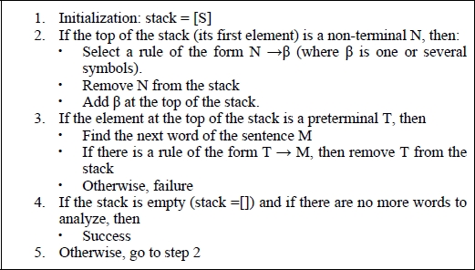
Figure 4.72. Basic top-down algorithms
Step (1) of the algorithm initializes the stack with the special non-terminal symbol of the grammar, i.e. S. Step (2) searches for a rule in which the left-hand side is equal to the symbol which is located at the top of the stack. In the event of a success, it replaces this symbol by the non-terminal symbols that are located in the right-hand side of the rule. In our example (Figure 4.72), in step (b), the algorithm has searched for a rule in which the right-hand side is the symbol S, located at the top of the stack. It is the rule: S → NP VP. Then, S is removed from the stack and the symbols NP and VP are added. Step (3) deals with the case where a preterminal symbol, T, is located at the top of the stack. A preterminal symbol is a symbol which is rewritten in a terminal symbol. In other words, it is a morphological category (noun, determiner, verb, etc.). In this case, the algorithm tries to find a rule that has the preterminal symbol in its left-hand side and the next word of the sentence in its right-hand side. In the event of a success, the algorithm removes T from the stack; otherwise, it declares its failure. If we go back to our example in Figure 4.71, the preterminal symbol is Det and it is associated with success in the next word of the sentence the (in this case, it is the first) which is a determiner and this thanks to the rule (Det → the). Step (4) is the stop condition of the algorithm. In fact, for the algorithm to succeed, two conditions must be met: the stack must be empty and all the words in the input sentence must be parsed. In our example (Figure 4.71), the algorithm terminates with success in step (4) because, on the one hand, the stack is empty and, on the other hand, all the words in the sentence are parsed. The last step (5) allows the algorithm to loop until it arrives at a point where it declares its success or failure.
The question now is how our parsing algorithm will process syntactic ambiguities. In reality, both bottom and top parsing algorithms can adopt one of three exploration strategies to process ambiguities: backtracking, determinism and breadth-first search.
In our presentation of the top-down parsing approach, we have adopted an exploration strategy which is called backtracking or the Depth-First Search. This strategy is to develop a single rule even when the grammar offers several possible rules at a given point of the parsing. If the algorithm arrives at a parse that is not compatible with the sentence in the course of the parsing, it reverts to (it performs a backtracking) the first not explored alternative and it modifies the parse by adopting a new possible rule. To illustrate this mechanism, suppose that the input of our parsing algorithm is: John likes the book. The algorithm will first try to analyze the subject noun phrase with the rule (NP → Det N). Such an attempt will fail in step (3) of the algorithm because John is not of the category Det. Backtracking requires choice points to be marked (e.g. stored in a data structure), to be able to cancel everything up to the last choice point in the event of a failure. This is not necessary in the case of programming with Prolog language, where the backtracking mechanism is natively implemented.
As backtracking has a non-negligible calculation cost, some researchers have explored the possibility of a deterministic strategy. In fact, the intuitive observation of the human parsing process shows us that the resolution of ambiguity is not performed by a research of the set of rules applicable to the sentence in the course of processing. To do this, humans seem to use all the knowledge they have to choose the solution that seems most plausible. The arguments in favor of this type of strategies are the extreme speed of the human parser and the non-conscientization of different possibilities as humans can interpret sentences without realizing the existence of several possibilities. This intuitive observation has given birth to several algorithms including those by [MAR 80] and [SAB 83].
Another control strategy, which is called breadth-first search, is to explore all possible rules at all points in the parsing. It is a horizontal exploration of the search space that allows us to identify all possible parses of a sentence in the case of a syntactic ambiguity. Such a strategy allows the à posteriori selection of the best parse according to syntactic, semantic, discursive, etc. criteria. From a cognitive point of view, such a strategy is not relevant, because humans do not seem to consider all possible analyses of a sentence at the same time. With respect to the computational point of view, this strategy is very costly in terms of space (memory) and parsing time. This is particularly true with actual applications where the grammar size is quite large, and sometimes it makes possible an infinite number of parses for a given sentence.
The problem of the left recursion is very often cited in the literature as the main limit of top-down algorithms, because of the rules of the form: A → A α will cause this algorithm to loop to infinity. To illustrate this problem, let us take the micro-grammar of the Figure 4.73.

Figure 4.73. Micro-grammar with a left recursion
To analyze any sentence with the grammar of the Figure 4.73, the algorithm will first try the first rule S → NP VP and then it will try to develop the noun phrase with the rule NP → NP PP and it, therefore, falls in an infinite loop, as illustrated in Figure 4.74.
To resolve this problem, we could perform transformations on the form of the rules, but this will not provide linguistically relevant parse trees (see [GRU 95] for more details on this issue).

Figure 4.74. Left recursion with a top-down algorithm
4.4.4. Bottom-up approach
Unlike top-down algorithms, bottom-up algorithms begin with the words and then go up gradually to achieve a parse of the entire sentence, if it is possible. It consists of searching for the words of the sentence and then combining them together in higher order structures by using the grammar rules until the arrival at the axiom. The stack in the bottom-up algorithms contains the symbols that have already been parsed.
The simplest bottom-up algorithm is called shift-reduce. As indicated by its name, this algorithm is based on two operations:
- – shift: allow the algorithm to move to the next word;
- – reduction: try to combine the constituents already found in higher constituents. This operation is possible thanks to a stack which retains the already found constituents.
Continuing with our sentence: Le livre est intéressant (The book is interesting) and the grammar of the Figure 4.70 we get the parsing steps presented in Figure 4.75.

Figure 4.75. Example of parsing with a bottom-up algorithm
The steps of the shift-reduce algorithm are provided in Figure 4.76.

Figure 4.76. Basic top-down algorithms
The bottom-up algorithm provided in Figure 4.76 is based on the two operations that we have just presented. There are two alternatives of which only one is applied at a given point of the analysis.
If we go back to our example in Figure 4.75, the algorithm firstly begins the parsing with an empty stack. With the shift operation, it takes the first word of the sentence the, and it finds its grammatical category det that it puts in the stack (Step A). As there is no grammar rule in which the left-hand side is the non-terminal det (the unique symbol in the stack), the algorithm performs another shift: it finds the grammatical category N of the next word book and it adds it to the stack that now contains the two symbols Det and N (Step B). The algorithm finds a rule whose right-hand side is: Det N. It is the rule: NP → Det N. It performs a reduction which is to remove the two symbols that are located in the right-hand side of this rule of the stack and to replace them with the symbol which is located in its left-hand side: NP (Step C). Finally, in step (g), the two conditions of success are met: the algorithm has consumed all the input words and it has only the symbol S in the stack.
It is probably necessary to note finally that the top-down approach includes several commonly used parsing algorithms, such as CYK, EARLY [EAR 70] and GRL [TOM 86].
4.4.5. Mixed approach: left-corner
Historically attributed to [IRO 61, GRI 65] and [ROS 70], the left-corner approach is a hybrid approach that combines the methods of two approaches that we have just seen: the bottom-up approach and the top-down approach. This is performed in order to increase the efficiency of the parsing by reducing the search space.
The motivation behind the creation of this algorithm can be explained with the following example. Suppose that our algorithm has the fragment of grammar of the Figure 4.77 and that we have to parse the French interrogative sentence: vient-il (is he coming)?

Figure 4.77. CFG Grammar
To analyze the input sentence, a top-down algorithm will perform the steps shown in Figure 4.78.

Figure 4.78. Repeated backtracking with a top-down algorithm
As we see in Figure 4.78, the algorithm starts to construct the tree from its root S. According to the grammar, a sentence can have two forms, thus the algorithm starts with the first (S → NP VP) (Step B). Then, on three occasions, it tries to find the noun phrase (Steps C, D and E) without success. In that case, due to the lack of other opportunities, it backtracks and tries the second form of the sentence (S → VP NP) which will eventually lead to the correct parse. In other words, to find the parse, the algorithm has performed four backtracks and this in a mini-grammar, then we can imagine the cumbersome nature of the research with a grammar of a large size.
Intuitively, we can say that the bottom-up approach is not cognitively relevant, because humans do not seem to examine all possibilities mechanically. In fact, a normally constituted human would move immediately to the second form of the sentence (S → VP NP), simply because the noun phrase cannot begin with a verb. This idea is the basis of the left-corner algorithm which uses precompiled tables of words or of grammatical categories that can appear at the beginning of a constituent. If we go back to our grammar of the Figure 4.70, a table of category and of lexicon can have the form provided in Table 4.10.
Table 4.10. Table of left-corners of the grammar of the Figure 4.70
| Category | Left-corner (categories) | Left-corner (lexicon) |
| S | Det, NP | the, my, John |
| NP | Det, NP | the, my, John |
| VP | V | is, loves, descends |
As we can see in Table 4.10, two types of information can be stored in the table: grammatical categories or lexical units. Depending on the size of the vocabulary, one of these choices is appropriate. In fact, in the case of a very large vocabulary as in the automatic translation applications of open texts, the compilation of a vocabulary with tens of thousands of words could cause memory problems for the system. In this case, we prefer the grammatical categories, in spite of the cost in terms of calculation.
Obviously, a rule which passes the lexical filter does not necessarily apply successfully, but this simply serves to reduce the search space and therefore increase the effectiveness of the algorithm.
A left-corner parser recognizes the left corner of a rule in a bottom-up fashion and predicts the rest of the symbols in the right-hand side of a rule in a top-down fashion. It includes three principal operations: shift, prediction and attachment.
Similar to the operation of the same name that we have just seen at the bottom-up algorithm, shift is to identify the category of the next word in the sentence (or the first word at the beginning) and to place in the stack the category which has been found. Prediction is to predict a constituent from its siblings. For example, suppose our stack has an NP at its top which corresponds to an already found noun phrase and that our grammar contains the rule (S → NP VP), then the NP will be replaced with S/VP. This means that the algorithm has predicted an S and that it must find the VP for the parsing of S to be successful. Attachment, meanwhile, is performed in two forms. The first is to consider a predicted constituent as already found when we find its constituents. For example, when we arrive at identifying an already predicted VP, the stack could have a form like [VP, S/VP]. Logically, the previous stack will be reduced to the form [S]. The second form is to combine the predictions that intersect. Thus, when we need to find an NP (complement) to complete a VP and if the latter is in turn necessary to complete a S, then we can deduce that we need an NP to complete S. The stack will be updated in the following manner: [VP/NP, S/VP] => [S/NP]. Note that a predicted element without having found any of its constituents will be noted as X/.
A possible form of the left-corner approach is provided in Figure 4.79. In fact, as the left-corner approach is a general strategy, it has been applied to various parsing algorithms such as GLC [NED 93], RTN [KUR 03] or tabular parsing [MOO 04].
Continuing with our example: Le livre est intéressant (The book is interesting) analyzed with the grammar 4.70 and the left-corner algorithm of the Figure 4.79, we get the steps presented in Figure 4.80. First of all, the algorithm predicts in a top-down approach that it is parsing a sentence and that is why it places the symbol S/ in the stack (Step A). In Step (b), it performs a shift by analyzing the left-corner of the sentence, the determiner The (Le), of which it finds the category (Det) that it places in the stack. With the rule (NP → Det N), it predicts that there must be a noun N to complete the already initiated NP and the stack is updated to reflect the new waiting expectation. Next, in step (c), after having found the N, it adds it to the stack. In step (d), it attaches the two constituents of the found NP. In step (e), it predicts a VP from the rule (S → NP VP) and the stack becomes [S/VP]. In other words, it announces that it has already found an NP to complete the predicted S and that it requires the VP. In step (h), it performs an attachment and then it declares the parsing successful; as the stack contains the symbol S and as all the words in the sentence have been consumed.

Figure 4.79. Left-corner algorithm

Figure 4.80. Example of parsing with the left-corner algorithm
In addition, several studies in computational psycholinguistics have shown that the top and top-down algorithms present difficulties as regards the processing of cases of left-branching and right-branching, respectively [JOH 83, ABN 91b, RES 92a]. This is due to the need for storage of intermediate information before being able to analyze the entire sentence. A summary of the spaces required by the three types of algorithms is provided in Table 4.11.
Table 4.11. Summary of spaces required by the three parsing approaches [RES 92a]
| Strategy | Required space | ||
| Left | Auto | Right | |
| Bottom | O(n) | O(n) | O(1) |
| Top | O(1) | O(n) | O(n) |
| Left-corner | O(1) | O(n) | O(1) |
First of all, note that n in Table 4.11 represents the width of the trees in terms of nodes and that O(1) represents a fixed processing time. Just like humans, the three strategies require more space to process the self-embedding structures regardless of their embedding degree. By contrast, we find an asymmetry in the processing of sentences with left-branching and right-branching for bottom and bottom-up algorithms. However, humans do not seem to process these two forms asymmetrically. This is considered as an argument in favor of the cognitive plausibility of the left-corner approach.
The left-corner approach cannot prevent the activation of irrelevant rules with respect to the context, particularly in the case of homography where two words with the same graphic form correspond to different grammatical categories such as the words plant and use which belong to both categories: verb and noun. In addition, the rules which do not have a left-corner, because their right-hand side is null (e.g. A → ϕ), require a particular processing. In contrast to the top-down approach, the left-corner can parse the left recursive rules to the left without looping to infinity, particularly thanks to lexical filtering.
4.4.6. Tabular parsing (chart)
Historically, the authorship of tabular parsing, which is commonly called chart parsing, is attributed to Martin Kay [KAY 67]. It is based on a dynamic programming approach, in which the main idea is the storage of the partial results found in the intermediate steps in order to reuse them in a subsequent step. The algorithm parses the same piece only once, which makes it more effective. Tabular parsing can be combined with the three parsing approaches that we have just seen, the top-down approach, the bottom-up approach and the corner-left approach. Similarly, it can use breadth-first or depth-first search strategies.
Tabular parsing is often compared to similar approaches, including the Earley algorithm and the Cocke–Younger–Kasami algorithm (CYK) [EAR 70, KAS 65, YOU 67]. Given the importance of this type of algorithm, several books have devoted large sections to it with detailed presentations including [VIN 83, GAZ 89, BLA 09, COV 94].
To store intermediate parses, it uses a data structure called chart. It is a set of nodes linked by edges. Each word of the input sentence is surrounded by two nodes that are marked by numbers. The edges at their turn mark the constituents. Let us take a look at the table of Figure 4.81 as an example.

Figure 4.81. Table of an incomplete parsing
The table presented in Figure 4.81 contains numbers between 0 and 6 which surround the words of the sentence from the beginning to the end. The edges have the function to indicate the structures which have already been recognized by the parser. In our case, two edges mark a proper noun and an NP between 0 and 1 and an edge marking a verb between 1 and 2. As for the progress of the parsing, the parser adds new edges to the table to account for identified constituents. Note that in the case of an ambiguity of morphological or syntactic category, the table contains two edges which connect the nodes which surround the ambiguous word with two different labels.

Figure 4.82. Table of a complete parsing of a sentence
At the stage of parsing presented in Figure 4.82, the algorithm stops with success because, on the one hand, all possible edges between 0 and 6 are filled with an edge with the category S and, on the other hand, all the words in the input sentence had been analyzed. We also note that some elements are marked at several levels. For example, John is both a proper noun NP and a noun phrase NP and it is also a part of the sentence S.
The table in Figure 4.82 is a particular case that we commonly call “passive charts”, because they do not realize the previously completed analyses that are partial or complete.
Active charts are the other type of tables which consists of realizing the state of parsing in a more comprehensive manner, i.e. what has been performed, as well as planned projects or steps. Concretely, an active chart contains active edges, i.e. edges whose requirements are only partially satisfied, as well as an agenda that defines the priority of task execution.
Active edges or dot rules are ordinary rewrite rules, but with an additional dot in their right-hand side that separates what has been analyzed from what has not been analyzed, or from what we call the rest. For example, the rule (S → NP • VP) indicates a situation where a noun phrase was found and where it requires a verb phrase to complete the parsing of the sentence.
If we go back to our example, Le livre est intéressant (The book is interesting) and the grammar of Figure 4.70, we get the active chart of the Figure 4.83.

Figure 4.83. Partial active chart
As we can see in Figure 4.83, we have two equivalent representations of the parse table with two active edges and a passive edge. The interpretation of this table is as follows. First of all, the parser predicts a constituent of NP type without recognizing any element (the dot is located at the right end of the right-hand side of the rule) and then after having identified a Det (marked by a passive edge), it moves the dot to the right of the identified constituent in the new initiated active edge. The question that now arises is how to combine passive edges with active edges to account for the progress of the parsing. To do this, tabular analyzers have a fundamental rule.
The intuition behind the fundamental rule is very simple. As an active edge expresses an expectation of specific constituents in a given context, the state of this expectation must be updated with the progress of the parsing and the discovery of one of these constituents that are expressed by the addition of a passive edge. This modification is performed simply by the advancement of the dot to the right of the symbol found in the rewrite rule. A more formal presentation of this rule is provided in Figure 4.84.

Figure 4.84. Diagram of the first fundamental rule
Let us take a concrete example: the sentence Le livre est intéressant (The book is interesting) analyzed with the grammar of the Figure 4.70 (Figure 4.85).

Figure 4.85. Example of application of the fundamental rule
The example presented in Figure 4.85 contains a labeled active edge (S →NP • VP). This means that the parser is expecting a VP. The following passive edge indicates that we have already found the VP initiated by the active edge. The fundamental rule allows us to combine the two edges and to advance the state of parsing considering that the sentence S has been fully parsed by generating an active edge labeled with (S →NP VP •).
To operate normally, a parser with an active chart must use an agenda. It is a data structure that allows us to plan the actions. In other words, the agenda of a tabular analyzer plays a similar role to the stacks that we have just seen: to memorize the actions and to establish priorities9.
In sum, tabular parsing, by storing partial results, avoids repeating the same parsing several times by performing backtrackings (as is the case with the simple algorithms that we have seen). Similarly, we have seen that this approach has an effective mechanism for processing ambiguities. It is probably necessary to mention that parsers of this type do not have a problem with the left recursion that is either with a top-down or a bottom-up strategy.
However, the addition of predictions to the parse table, the main advantage of tabular analyzers, has a few disadvantages. In fact, with either a top-down or a bottom-up strategy, this could mislead the parsing with incorrect predictions.

Figure 4.86. Tabular parsing algorithm with a bottom-up approach
4.4.7. Probabilistic parsing
The idea behind statistical parsing is to combine the discrete symbolic information with the statistical information of a continuing nature. In practice, this is to enrich the existing linguistic formalisms with statistics obtained from corpora related to application fields [CHA 93a, BOD 95, ABN 96]. The way in which the Probabilistic CFG (PCFG) extends the CFG is often compared to the extension of regular grammars by the HMMs that we have seen in Chapter 2. The objectives of these different approaches can be summarized by ambiguity resolution, as well as the limitation of the search space of classical parsing algorithms. Studies in this context have been performed in two complementary axes: the definition of statistical formalisms, as well as the proposition of algorithms.
The definition of probabilistic formalisms, in the general case, is to propose probabilistic versions of existing formalisms. We can mention in this framework the studies on probabilistic CFGs [JEL 92], stochastic LTAG [SCH 92, RES 92b], stochastic LFG [BOD 00, BOD 98], etc. Sometimes, probabilistic analysis is proposed for the resolution of specific problems, such as processing of syntactic discontinuities [LEV 05] or ambiguity resolution [TOU 05]. The main problem addressed by these studies is the hierarchization of probabilities according to linguistic units. Thus, we distinguish between internal probabilities, within the basic linguistic unit such as the phrase and the chunk and inter-unit external probabilities.
The other axis consists of the proposition of algorithms for probabilistic analysis. In this context, we can mention the studies by [MAG 94, BOD 95, GOO 98], etc. The main issues targeted on this axis are the obtaining of the most probable parse tree (ambiguity resolution) effectively, the learning automation of PCFG, as well as the reduction of the size of the learning corpora.
The probabilistic analysis is a method which has several benefits for the processing procedure, but its practical realization is generally difficult, particularly in the context of deep parsing systems, especially because of the need for a large quantity of correctly pre-parsed data.
From a formal point of view, a PCFG grammar can be defined as G = (VN, VT, S, R, Π). The only difference compared to the definition of the CFG that we have seen is the element Π which is the set of probabilities associated with production rules with: π(α→β) 0 ≥ where α→β ∈ R.
As we note in Figure 4.87, the sum of probabilities of the rules which share the same non-terminal symbol in their left-hand side is equal to one. More formally, we can say that the PCFG obey the property formulated by the following equation: ![]() . For example, if we take the case of rules of NP: π(NP → Det N) + π(NP → PN) + π(NP → Pron) = 0.27 + 0.63 +0.1 = 1.
. For example, if we take the case of rules of NP: π(NP → Det N) + π(NP → PN) + π(NP → Pron) = 0.27 + 0.63 +0.1 = 1.

Figure 4.87. Example of a probabilistic context-free grammar for a fragment of French
To calculate the probability of an parsing tree, simply multiply the probabilities of the rules used in its derivation, as we assume that the probabilities of the rules are independent. Thus, the probabilities of trees a1 and a2 in Figure 4.88 are calculated in the following manner from the grammar of the Figure 4.87:

As we note, logically, the larger the parsing tree is, the smaller its probability is.

Figure 4.88. Parsing tree for a sentence from the PCFG of the Figure 4.87
In the case of the two sentences of Figure 4.88, each sentence is associated with a single parse, as there is no syntactic ambiguity. What is interesting about a probabilistic grammar is that it assigns a probability to all analyses or possible derivations of a syntactically ambiguous sentence, allowing us to resolve the ambiguity. More formally, suppose we have a sentence S which is likely to receive n different parses, the probability of this sentence can be calculated according to the equation [4.33]. Thus, for each derivation d member of the set of derivations of S, we have a probability associated with this derivation τ(S). The probability of a sentence is equal to the sum of the probabilities of its derivations.
Despite its benefits, PCFG suffers from several well-known limitations in the literature. In fact, according to the independence hypothesis, each rule is independent of other rules which constitute the parsing tree. Thus, the rule S → NP VP does not imply any limitation with respect to the form of the subject noun phrase. However, studies such as [FRA 99] have shown that in English in 91% of the cases, the subject NP is a pronoun. In addition, conjunction ambiguities as in [4.16a] are impossible to solve with a PCFG, since the two possible parses have the same ambiguity. To resolve these problems, several strategies have been proposed in the literature. The simplest strategy is to differentiate labels. For example, rather than having the category NP, we would have NP_Subject and NP_Object. A more linguistically motivated solution is to lexicalize the grammar and to associate probabilities to lexically anchored trees. This allows us to take into consideration several syntactic parsing levels.
In a practical manner, PCFGs are inferred generally from a syntactically annotated corpus, which is often called TreeBank (see Figure 4.89 for a describing this process). The inference algorithm explores the trees in the corpus and calculates the probabilities of each of the rules observed by using the [4.34].

Figure 4.89. Supervised learning of a PCFG
Another approach is to infer the PCFG from a non-annotated corpus. Typically, we use the inside-outside algorithm whose principle is similar to the Baum-Welch algorithm for the estimation of the parameters of an HMM. As we might think, these studies are still at the research stage and their performance is still inferior to that of the supervised approach.
Several probabilistic parsing algorithms have been proposed, many of which are inspired by the tabular parsing approach described in section 4.4.6. To find the best parse among the possible parses, algorithm such as A* or Viterbi, that we have presented in Chapter 2, are used [COL 99, KLE 03].
To give a concrete idea of the probabilistic syntactic parsing, let us take the CYK algorithm as an example. Named after its historical inventors, Coke, Yonger and Kasami, this algorithm is a tabular algorithm which follows a bottom-up approach. It requires grammars in Chomsky normal form, in which all rules above the preterminal level are binary. Effective, this algorithm has a processing time complexity which is equal to O(n3) and requires a space of O(n2). As it follows a dynamic programming approach, this algorithm searches for all partial parses for the sequences of equal length up to n words where n is the number of words of the input sentence. The probabilistic version of this algorithm uses the same approach, but it is distinguished by the association of a probability to each sequence produced by a rule (see [CHA 98] for an example). If we take as an example the French sentence Le livre est intéressant (The book is interesting) with the grammar 4.87, we get the following parse steps. The first step is to create a data structure which is called table or parsing triangle, as it has the shape of an inverted right triangle whose two catheti are formed by n cells where n is equal to the number of words of the input string. As we can see in Figure 4.90, each cell covers a substring with a beginning index and an ending index.

Figure 4.90. General structure of the parse table of the CYK algorithm
The parsing algorithm proceeds by filling the hypotenuse of the rectangle with the information on the morphological categories of input words introducing the rules of the form: preterminal → word (see Figure 4.91). Lexical ambiguities are retained to the extent that we add the different parsing possibilities of a word with their probabilities. For example, for the word le (the), we add the two possible rules in the grammar: Det → the 0.55 and Pron → the 0.3. Next, the algorithm searches if there are higher level structures which have the preterminal used to the right-hand side. For example, we find that it is possible to construct a noun phrase with the following rule: NP → Pron. The probability associated with this rule in the parse table is calculated as follows: π(NP → Pron) * π(Pron → the) = 0.1*0.3=0.03.

Figure 4.91. The first step in the execution of the CYK algorithm
In the second diagonal line, the algorithm searches for strings of two words by combining the representations which have already been constructed at the previous level, that of words (see Figure 4.92). For example, it finds that it is possible to construct a sentence with the rule S → NP VP [0, 2] whose probability is calculated in the following manner: π(S → NP VP) π(NP → Pron) π(VP → V) = 0.7*0.0006*0.051 = 0.000021. In a similar manner, the algorithm discovers the possibility of obtaining a sentence in the cell [2, 4]. The cell [1,3] remains empty because the string livre est (book is) does not correspond to any constituent.
In the third step, the algorithm finds the possibility to construct a sentence with the rule S → NP VP in the cell [0.3] (Figure 4.93).

Figure 4.92. The second step in the execution of the CYK algorithm

Figure 4.93. The third step in the execution of the CYK algorithm
Finally, the algorithm finds a rule whose left-hand side is p and which covers the entire sentence in the cell [0, 4] (Figure 4.94). This allows us to conclude that the string Le livre est intéressant (The book is interesting) is a legitimate sentence according to our grammar. In the case of ambiguity, i.e. two different rules with the same non-terminal symbol in their left-hand side and which cover exactly the same string, we keep only the most probable rule. This is the mechanism that allows the CYK algorithm to resolve the ambiguity.

Figure 4.94. The fourth step in the execution of the CYK algorithm
To find the parse tree, we must enrich the rules with indexes to indicate the extent of each constituent. For example, the rule S → NP VP in the cell [0,4] will be marked in the following manner: S → NP [0,2] VP [2,4].
4.4.8. Neural networks
As we have seen in the sphere of speech, the first investigations on neural networks were presented in the 1940s with the studies by Walter Pitts and Warren McCulloch. After a series of partial successes and failures, neural networks have begun to occupy an important place in the landscape of artificial intelligence in the general sense of the term from the 1980s, particularly following the publication of the book parallel distributed processing by David Rumellheart and his collaborator [RUM 86] (see [JUT 94] and [JOD 94] for an introduction).
Today neural networks bring together an important family of statistical learning algorithms. Some of them, such as perceptrons, follow the supervised learning mode where the network learns by comparing the given input with the correct classification. Other networks adopt a non-supervised learning mode such as Kohonen maps or self-organizing maps (SOM) [KOH 82].
To be concrete, let us take the example of multilayer perceptrons which are a popular form of supervised neural networks. The architecture of this system is composed of three parts: the input layer, one or several hidden layers and the output layer. The input layer has the function of introducing the coded data to the network. For example, in the task of handwritten digit recognition, this layer can consist of n neurons where n is equal to the number of pixels of the images of each digit. Thus, with images of 28 × 28 pixels, we must have 784 neurons in the input layer. The hidden layer, in turn, constructs an internal representation within the network. Finally, the output layer corresponds to the classes of our system which, in the case of digit recognition, are ten (see network architecture in Figure 4.95). Each neuron in the network is connected to a subset of neurons in the network. Each connection has a weight whose value can change during the learning process. Neurons also have an activation function f which controls their outputs given their inputs. The input of a neuron is the weighted sum of neuron outputs of which it receives the output. The complexity of this function varies depending on the networks. The simplest function is called identity function, where the output of a network is equal to its net input: f(x) = x. In this case, we refer to a linear network. More complex activation functions are also used depending on applications such as the step function with f(x) =0 if x ≤ 0 and f(x)=1 if x > 0 or the sigmoid function:

There are two different but complementary forms of learning in a neural. The first one is to store diverse information in a compact form, such as in a Hopfield network [HOP 82]. The second method is to deduct forms of implicit rules that generalize the cases observed in the concrete examples provided in learning.

Figure 4.95. Architecture of a neural network for handwritten digit recognition [NIE 14]
The main limitation to applying networks such as the one in Figure 4.91 is the lack of consideration of context, since digits are recognized only based on their content. To take into account contextual information and temporal sequences, Elman has proposed a particular architecture of neural networks called recurring networks [ELM 90]. Unlike traditional networks, where the flow of information always goes forward: from the input to the output, feedforward, the recurrent networks allow for a return of information rearward. Inspired by the biological neural networks, this bidirectionality allows us to account for the context by memorizing implicitly one or several history stages (see Figure 4.96).
This type of network has been the subject of several studies for the construction of artificial neural networks which are capable of performing syntactic parsing effectively [JOD 93, HEN 94, GER 01] (see [HEN 10] for a review of these studies).

Figure 4.96. Example of a recurring network
Despite their interest, the results with neural networks were often inferior to those of statistical approaches. Even in the case of comparable performance, as for speech recognition, neural networks have been disadvantaged because of the high cost of learning. In fact, for actual applications learning required sometimes weeks, which means that researchers had a very low margin of error. A consequence of this cumbersome nature of learning was the inability to equip networks with the appropriate number of hidden layers to construct rich enough internal representations, because the addition of new internal layers dramatically increases learning time. To resolve this problem, a group of Canadian researchers including Geoffrey Hinton have proposed a new paradigm named deep learning [HIN 06, HIN 12] (see [BEN 09] for an introduction). This has opened the way for the exploration of new architectures of neural networks to solve a fairly large number of problems including the tricky problem of parsing.
Thus, several studies have focused on building syntactic parsers with this new type of neural networks. Typically, these studies focus on dependency formalisms [COL 11, ETS 13, CHE 14].
4.4.9. Parsing algorithms for unification-based grammars
Unification grammars, as we have seen, contain complex feature structures. We have also seen a simple way to process the additional information encoded by the features in the framework of DCG.
Let us go back to the tabular parsing algorithm to examine how it can be adapted to parse unification-based grammars. The principle is simple: in addition to the constraints on the grammatical categories imposed by grammar, the parser requires the unification of features associated with each example. It is therefore an addition of new constraints.
If we assume that the algorithm adopts a top-down approach, then it will first predict an active edge of the form:

In the previous rule, the noun phrase and the verb phrase have a reentrant feature to ensure the agreement of the verb with its subject. Next, by processing the word John, it will add the following passive edge where we have voluntarily simplified it by considering that a proper noun is directly sufficient for a noun phrase:

With the fundamental rule, we advance the point to the right of the symbol.

The rest of the sentence is processed in the same way until obtaining a complete parse: all words are covered under the category S. Note that, in addition, the algorithm must verify the unification of the reentrant features to ensure agreement.
4.4.10. Robust parsing approaches
A robust parser is a system that is able to provide a correct parsing tree even in the case of an incomplete, distorted or unexpected input. Several robust parsing techniques have been developed in the framework of studies on the spoken, as well as on the written language. In both cases, the objective is the use of parsing algorithms in actual conditions: recognition errors and speech extragrammaticalities for spoken language and typing errors and grammatical errors in written texts. The main techniques used in robust parsing consist of extensions of conventional parsing algorithms, in order to energize them and make them more appropriate to unexpected actual applications. In addition, some approaches are based on studies in fields such as information retrieval and document classification.
4.4.10.1. Chunk parsing
Inspired by the studies of [GEE 83] in psycholinguistics, [ABN 90, ABN 95] proposes a partial parsing approach based on the segment (chunk parsing).
In a chunk parser, parsing is divided into two completely distinct parts (unlike the traditional approaches in which the two steps are merged):
- – segmentation: the conversion of the flow of words in a flow of segments;
- – attachment: the attachment of the segments obtained in the previous phase within a global structure, which is the parse tree of the utterance. In regard to the previous part, this step is not mandatory or at least not systematic. Thus, a chunker can provide complete parsing trees and partial segments or only partial segments.
Cascaded parsing of syntactic structure (CASS) is a robust parser system based on chunks. This system has been developed by Steven Abney at the University of Tübingen in Germany. CASS uses a set of simple parsers that apply in cascade to construct a global syntactic representation of the utterance.
The input of CASS is the output of Church’s tagger [CHU 8] which provides POS tags to the words, as well as the simple (non-recursive) noun phrases. Note that the processing rate of noun phrases is lower than that of POS tags. The processing of the pre-processed input in CASS is performed according to three steps: the chunk filter, the clause filter and the parse filter.
In turn, the chunk filter is based on two subfilters: the noun phrases filter and the chunk filter. The noun phrases filter is a module which uses regular expressions to assemble noun phrases based on the superficial analysis provided by Church’s noun phrase recognizer. Similarly in this module, we correct the processing errors of noun phrases by the Church’s module, such as those resulting from prenominal adjectives. In addition, the chunk filter also uses regular expressions to recognize the rest of the segments. Here is an example of the output of this module with the utterance: In south Australia beds of Boulders were deposited.

As we can see, the system has committed an error of parsing (because of the tagger) of the first noun phrase south Australia beds.
The clause filter also consists of two subfilters: the raw filter and the corrected clause filter. The raw filter tries to recognize the boundaries of simple clauses, as well as marking the subject and the predicate of the clause. If it is unable to identify a single subject or predicate, this module identifies the type of error encountered, such as the existence of several verbal phrases or the absence of a subject (because of an ellipsis, for example), etc. In addition, the corrected clause filter is a module that tries to correct the errors identified by the previous module by applying specific patterns in each case. For example, the following is the pattern used for the correction of non-analyzed complementers: [pp Xp-time NP] … VP → [clause Xc NP ... VP]. In cases where none of the patterns are applicable to the input, the system uses general heuristics that allow it to improve the analysis based on partial information (such as the existence of a noun phrase next to a verb phrase, only a verb phrase, etc.). Thus, after this step, the parse obtained for the utterance becomes as follows:

As we can see in the previous parse, the system has succeeded in correcting the error of parsing in the first phrase.
Unlike the previous modules, the parsing filter is based on recursive rules (not regular expressions). The main function of this module is to assemble recursive structures by attaching the nodes to each other according to the nature of the heads of these structures and the grammatical constraints on their assembly. For example, a segment Y can be attached to a segment X only if the head of X can have Y as an argument or modifier.
The results of CASS have shown that it is both robust enough and very fast for the processing of written corpora. These results are mainly due to the architecture of the system which is to apply different parsing levels in cascade with rules and patterns that allow us to correct the errors made in the previous steps.
Different approaches similar to Abney’s approach were proposed including that by [AIT 97, GRE 99] which is based on techniques of FSAs and that of supertagging proposed by [CHE 99, SRI 99], in the framework of LTAG formalism.
4.4.10.2. Selective approaches
Selective approaches, which are sometimes called island-driven parsing, consist of analyzing only the parties considered relevant or non-noisy by the received utterance. These approaches are supported by simple observations on human language and speech processing which is characterized by the variation of the degree of attention. From a computational point of view, it often refers to equipping the parsing algorithm with a filter which allows us, according to a number of constraints, to ignore one or more words or the non-parsable segments. In fact, when analyzing the oral language, the input of the parser is the output of the module for speech recognition which contains a variable error rate depending on the circumstances (the amount of noise, the speaker’s clarity of pronunciation, the richness of vocabulary, etc.).
Different degrees of selectivity have been used in the literature. This varies between fairly similar approaches to the parsing based on keywords such as [LUZ 87, ROU 00] to more reasonable coverage approaches such as the algorithm GLR* by [LAV 97] or the different implementations of semantic grammars at Carnegie Mellon University, as well as in other universities, [MAY 95, MIN 96, GAV 00, BOU 02].
Contrary to what some researchers in the field believe, selective approaches are not necessarily synonymous with information loss or shallow parsing. In fact, a well-designed selective strategy can be added to any parsing system without affecting its depth of analysis (see [KUR 03] for a more thorough discussion). The only drawback of these approaches is that they increase the computational complexity of algorithms to which they are added. For example, Wang [WAN 01] describes a chart parsing algorithm which is equipped with a selective strategy (for the parsing with a semantic grammar equivalent to CFG) whose complexity is O(b4) instead of O(b3), as is the case of several conventional algorithms for the CFG10.
4.4.10.3. Parsing of extragrammaticalities of the oral language
The presence of extragrammaticalities in the oral language makes the use of conventional algorithms such as those we have seen impossible. For example, during our spoken language study done on the Trains Corpus, a corpus of spontaneous oral conversations in American English, we have found that filled pauses or hesitations constitute approximately 7% of the words of this corpus and approximately 66,26% of the utterances contain hesitations, in addition to a significant number of more complex phenomena, such as repetitions, self-corrections and false starts. To overcome the difficulties of parsing related to extragrammaticalities of the oral language, several sources of knowledge have been used in the literature for the processing of extragrammaticalities, including structural information, morphosyntactic information, prosodic information.
Structural information focuses on the identity of each word and those of the words which follow them11. The advantage of this information is its reliability and simplicity of use, but its use is generally limited to the detection of repetitions with the help of patterns [SHR 94, HEE 97].
Morphosyntactic information essentially concerns the morphosyntactic categories of words or chunks and their possible successions. For example, the succession of two determiners is deemed extragrammatical and therefore the case is processed as an self-correction. Some systems have used more complex rules to model cases involving phrases. In these kinds of cases, conventional parsers have been developed to perform this task. These rules have generally been implemented as syntactic metarules in a post-processing module [COR 97, MCK 98, COR 99, KUR 02].
Prosodic information relies on a set of sources of various kinds, such as unfilled pauses and the melodic contour, which have been used to segment the input in syntactic constituents and therefore locate the center of the extragrammaticality in the utterance [NAK 94, LIC 94].
4.4.11. Generation algorithms
As we have seen with the parsing algorithms, the input is a string of words (typically a sentence) and the expected output of the algorithm is a description of syntactic properties of this input string as tree or a dependency graph. Then comes the role of semantic knowledge to provide an interpretation of the sentence. In the case of generation, it is the reverse process, because we must first consider what we would like to express in terms of semantic content and then we produce the syntactic structure from which we find the surface string. We can also consider a generation at the scale of an entire text where consideration of discursive knowledge is indispensable, particularly when taking into account the connections between the sentences. We refer to [DAN 00, REI 10] for a general introduction to the issues of syntactic and semantic generation. With regard to the syntactic aspects of generation, we often use top-down algorithms sometimes with a tabular algorithm. Unification is also used to control the forms of the sentences generated in many approaches including [GER 90, EST 90, REI 04].