
2
The Sphere of Speech
2.1. Linguistic studies of speech
The scientific study of speech, found at the intersection of a number of disciplines such as Physiology, Electronics, Psychology and Linguistics, is a very rich field. It forms the basis of a large number of practical applications, including speech pathology, language teaching and speech processing (SP), which is the focus of this chapter. Two key disciplines are at the heart of studies in this area: phonetics and phonology.
2.1.1. Phonetics
Phonetics is a field that deals with the scientific study of speech sounds. It provides methods for the description, classification and transcription of speech sounds [CRY 91]. As a branch of the natural sciences, it examines speech sounds from physical, physiological and psychological points of view. Phonetics involves making parallels between sounds in human language and looking at the physiological, physical and psychological constraints which have shaped these sounds. For a general introduction to phonetics, the reader can refer to a number of excellent works, including those of [LÉO 05, LAD 01, HAR 99, CAR 74].
Historically, the interest in describing the sounds of speech goes back to antiquity. It is widely thought that the Phoenicians developed the first system of phonetic transcription or alphabet on the east coast of the Mediterranean between 1700 and 1500 BC. The traces of this alphabet are still visible in some alphabets that exist today. As for the first actual phonetic descriptions, it is thought that they began in around 500 BC with the grammar of Sanskrit written by Panini, which contains a remarkable classification of the sounds of this language. In the Middle Ages, Arabic linguists carried out advanced research on descriptions of the sounds of Arabic, notably using a system of phonetic contrasts. Some of these works had a prescriptive objective, as the aim was to conserve the original phonetic form of the Quran’s message, eliminating changes which would take place throughout the ages [CRY 71]. Others, such as Avicenna’s work, had the aim of understanding the physiological basics of the process of speech production and, therefore, were more scientific in nature (see [KAD 04, WER 84] for a review of these works). In Europe, the interest in phonetics began to develop at the beginning of the 18th century, with the works of Joshua Steele, among others. It was in the 19th century, with Thomas Edison’s invention of the phonograph, that phonetics was able to make a large leap in progress. Thanks to this device, phoneticians were able to record spoken sequences and could describe their properties (by slowing down or speeding up the recordings). Among the works written during this period, we can cite those of Ludimar Hermann on the production of vowels.
Since it is much more practical to work with written forms, phoneticians developed a number of transcription systems for transcribing speech. In contrast to an ordinary alphabet, a transcription system is different because there is a direct and unique correspondence between a sound and its grapheme. Each individual sound corresponds to a single grapheme in the system of transcription and each grapheme is associated with one sound. Furthermore, a transcription system must be universal to be used to transcribe all the languages in the world. Among the systems of transcription, the International Phonetic Alphabet (IPA) is the best-known. It is a transcription system developed towards the end of the 19th century by the IPA. To examine the purpose of such an alphabet, let us examine Table 2.1, which presents some graphical forms in French for the sound [o] and some examples of transcription of the grapheme “o” in English.
Table 2.1. Examples of IPA transcriptions from French and English
| Word | Transcription |
| rose | [Roz] |
| chaud | [∫o] |
| Beau | [bo] |
| show | [ʃoʊ] |
| bond | [bαnd] |
| drone | [drəʊn] |
| ubiquitous | [jʊ’bɪkwɪt̬əs] |
The differences in grammatical forms are due to several reasons which can be morphological or even etymological. In spite of their apparent banality, the sounds of a language are far from being simple entities to study. Sounds can be studied from several points of view according to the specific location in the communication system (see Figure 2.1).

Figure 2.1. Communication system
This shows how the three main branches of phonetics are distinct: articulatory phonetics, which focuses on the production of sounds by the emitter; acoustic phonetics, which is located at the level of the transmission channel; and auditory phonetics, which focuses on the way in which the sounds are perceived by the receptor.
2.1.1.1. Articulatory phonetics
Articulatory phonetics takes the point of view of the emitter and considers the way in which sounds are produced by the speech organs such as the pharynx, the tongue and the lips. In other words, the physiology of the production of sounds is the true focus of this branch of phonetics.
To fully understand the process of the production of speech sounds, we can compare it to a well-known artificial process – the production of music by instruments. In both cases, we need a source which can be modified by a sound box of sorts. We are talking about a complex process involving a number of organs (the organs that make up the vocal tract) whose roles need to be coordinated efficiently. To explain this in a systematic way, these organs can be grouped into three functional components: the subglottic system, the phonatory system and the supraglottic (supralaryngeal) system (see Figure 2.2(a) for a global view of the speech apparatus and Figure 2.2(b) for a lateral view of the phonatory and supraglottic systems). Moreover, Broca’s area, situated in the frontal lobe of the cerebral cortex, can be considered as a major component of the vocal apparatus, because of the leading role that it plays in the coordination of this process. For more information on the process of speech production, see [MAR 07].
The subglottic system has the role of creating an air current following the deflation of the lungs after the diaphragm relaxes. Air freed in this way then moves across the trachea before arriving at the larynx. The main component of the production of sound, the larynx, is a cartilaginous solid structure which is situated above the trachea and below the middle part of the pharynx. Another specificity of the larynx is that it contains the two vocal folds which are two muscular bands of about 1 cm in length and 3 mm in width. During phonation, these folds come close to one another and begin to vibrate against each other. This vibration gives the sound its basic quality and is called the fundamental frequency. Think of vibration as happening in two modes: a heavy mode which produces deep sounds and a light mode for high-pitched sounds.

Figure 2.2. Speech organs
The articulation system, located above the larynx, is made up of three cavities which play an important role in the formation of sounds: the pharynx, the nasal cavity and the oral cavity. The pharynx is a cavity which resembles a tube whose main role is to connect the larynx with the nasal cavities and the respiratory tract as well as the mouth and the esophagus (digestive tract). The shape of the pharyngeal cavity determines the fundamental qualities which give a unique timbre to the voice of each and every one of us. With a fixed size and shape, the nasal cavity plays the role of the sound box, filtering the sound and producing resonances. In order for the air to pass through this cavity, the soft palate (velum) must be lowered (see Figure 2.3). If the lips are closed, the entire mass of air being released is directed through the nasal cavity, producing consonants like m. Likewise, the opening of the lips accompanied by the lowering of the soft palate produces nasal vowels such as the sound [ɑ̃] in French, for example in the word grand [gʀɑ̃].
The oral cavity is the most important of the three cavities, because of its total volume and also because of the number of organs which are found within it. It is made up of the palate, the tongue, the lips and the lower jaw.

Figure 2.3. Position of the soft palate during the production of French vowels
The palate, the upper part of the oral cavity, is separated into two parts: the hard palate and the soft palate. The hard palate, located in the bony frontal part, is immobile and its role is to support the tongue during its movements, therefore allowing for partial occlusions to be made. The soft palate or velum is situated further back.
The tongue is a complex organ made up of a collection of muscles which are responsible for its large range of mobility. It is divided into three main parts: the apex, the body and the root (see Figure 2.4).

Figure 2.4. Parts and aperture of the tongue
The distance between the body of the tongue and the palate or the degree of aperture allows the quantity of air which passes through the mouth to be controlled (Figure 2.5).

Figure 2.5. Degree of aperture
The lips, just like the tongue, are highly mobile and this allows them to assume many different shapes. Thus, when they come together, they create closure, for example when producing [m] or in the closure phase of [p]. On the other hand, when they are slightly open and round, they allow the production of vowels such as [o] and [u]. Likewise, when they are open and spread, they can produce vowels such as [i] and with a neutral position, they can produce [ə]. Finally, when the lower lip makes contact with the incisors, the sound [f] can be produced.
Ultimately, the lower jaw plays a moderating role by increasing or decreasing the size of the oral cavity.
2.1.1.2. Acoustic phonetics
Acoustic phonetics is a branch of phonetics which considers the physical properties of sound waves. Its focus is on what happens between the emitter and the receptor (see [MAR 08] for an introduction).
Let us begin by looking at the mechanism of production of sound waves. The movements of speech organs transmit a certain amount of energy to the air molecules surrounding them, creating a pattern of zones of high and low pressure, and we call this a sound wave. These waves propagate through the air (or, in some cases, through water), transmitting energy to neighboring molecules. To simplify the explanation of this process, let us look, for example, at the vibration of a tuning fork which causes the displacement of air molecules both forwards and backwards, as shown in Figure 2.6.

Figure 2.6. Displacement of air molecules by the vibrations of a tuning fork
As minimal units of communication, sound waves must be able to be perceptibly distinguishable from one another by virtue of their fundamental physical properties. These include frequency and amplitude differences which cause perceptual variations in tone (pitch) and volume (loudness), respectively (see Figure 2.7).
The frequency of a signal is measured in cycles per second or Hertz, while amplitude, also sometimes called intensity, is a measure of the energy transmitted by a wave according to a unit called the decibel. Note that a tuning fork does not vibrate infinitely but even if its amplitude lowers little by little, its frequency remains stable. This means that frequency and amplitude are completely independent from one another. In other words, we can have two different signals that have the same frequency but different amplitudes, or two signals that have the same amplitude but different frequencies.

Figure 2.7. Frequency and amplitude of a simple wave
Note that the wave shown in Figure 2.7 presents a certain regularity because it does not change shape as time progresses: the distance between the peaks is always fixed. This kind of wave is called a repetitive wave or a periodic wave. The waves of vowel sounds are waves of this type. However, another kind of wave does not produce this kind of regularity and is logically called a non-repetitive or aperiodic wave. This kind of wave corresponds to plosive sounds such as [p] or [b] or to clicks (see Figure 2.8).

Figure 2.8. An aperiodic wave
It is also useful to distinguish between simple waves and complex waves. Complex waves are the result of combining multiple simple waves. Consequently, it is possible to analyze a complex wave by looking at its simple components. As illustrated in Figure 2.9, the presentation of a complex signal (a) in the form of simple waves (b) does not allow us to show all the properties of its components. Therefore, it is necessary to use a more sophisticated instrument such as a spectrograph to do this.

Figure 2.9. Analysis of a complex wave
Before presenting the spectrograph, we shall consider the term resonance. Resonance is the transmission of a vibration from one body to another, namely the resonator. Note that each body has its own natural frequency that it reacts to with the most ease. Thus, a tuning fork that vibrates at 200 Hz will cause the vibration of another tuning fork if it has a natural neighboring frequency. A simplified way of seeing the spectrograph is to consider it as a collection of tuning forks, each with a different natural frequency. When these tuning forks find themselves next to a complex wave, some, whose natural frequency corresponds to the frequency of a simple component of this wave, will resonate, making it possible to carry out an analysis of this wave (see Figure 2.10).

Figure 2.10. A collection of tuning forks plays the role of a spectrograph
In Figure 2.10, we have a complex wave made up of three components which will make three tuning forks of the same frequency vibrate. These frequencies are 550 Hz. The information that is produced by a spectrograph is called a spectrogram. A spectrogram is a multidimensional representation of the sounds obtained with the fast Fourier transform. As shown in Figure 2.11, the vertical axis represents frequency, whereas the horizontal axis represents time. The dark zones in the spectrogram give information about concentrations of acoustic energy and these are called formants.

Figure 2.11. Spectrogram of a French speaker saying “la rose est rouge” generated using the Prat software
Formants play a fundamental role in the analysis of vowels where they are visible very clearly as vertical bars. To distinguish a vowel, it is normally sufficient to look at the first three formants. Table 2.2 presents the average values of the three first formants of the French vowels [a], [i] and [u].
Table 2.2. The three first formants of the vowels [a], [i] and [u]
| Formant | [a] | [i] | [u] |
| F1 | 750 | 200 | 200 |
| F2 | 1200 | 2200 | 700 |
| F3 | 2600 | 3200 | 2200 |
In general, F1 correlates with the size of the pharyngeal cavity. This explains why the F1 value of the vowel [a], which is an open vowel, is the highest. Likewise, the values of the first formant of vowels [i] and [u] are very low, because they are close vowels. F2 is generally associated with the shape and size of the oral cavity. In the case of the vowel [i], where the oral cavity is reduced in size, this causes a very high F2 level. In the case of the vowel [a], the openness and the large amount of space within the oral cavity causes a lower F2 value. When it comes to F3, it is possible to distinguish between the French vowels [i] and [y], where the lips play an important role ([y] being a front rounded vowel that is not used in English). When professional singers perform, the lowering of the larynx and the raising of the tongue causes the increase in F3 and F4 values, making them more prominent acoustically (see Figure 2.12).

Figure 2.12. Spectrograms of the French vowels: [a], [i] and [u]
When it comes to consonant sounds, several criteria come into play in order to describe their spectrograms. Criteria include the temporary transitions between formants, voicing1, periods of silence, etc. Let us examine Figure 2.13, where we will consider some examples of consonants produced alongside the vowel [u].

Figure 2.13. Spectrograms of several non-sense words with consonants in the center
As we can see in the spectrograms of Figure 2.13, the difference between the consonants [ʃ] and [s] can be seen by the position of the dark areas at the top of the spectrogram, reflecting the frequency of noise from friction which is much higher in the case of [s] than in the case of [ʃ]. The closure phase of the consonant [k] can be seen in the light area in the spectrogram followed by a little area of friction which corresponds to aspiration, a consequence of the release phase, since this is a voiceless consonant. The French fricative [ʁ] is seen as vertical bars of energy, which reflect friction. The nasal consonant [m] is characterized by a pattern that is similar to those of formants, shown as darker patches. Finally, the darker areas at the bottom of the spectrogram, which are visible for consonants [ʁ] and [m], reflect the fact that these consonants are voiced.
2.1.1.3. Auditory phonetics
Auditory phonetics is the study of how sounds are perceived, looking at what happens within the ear and also what happens when the brain is processing sounds. The study of auditory phonetics fits within the frameworks of work in physiology and experimental psychology (see [JOH 11, RAP 11] for a general introduction).
Before looking at the perception of speech sounds, let us consider the anatomy involved in auditory perception. Instead of focusing on the complexities of the multimodal perception of speech sounds (which involve parallel auditory and visual pathways), we will focus solely on the auditory pathway; we recommend [MCG 76] and [ROS 05] for more information on multimodal perception.
The auditory pathway is made up of three main parts: the ears, the cochlear nerve and the brain. The ear is the main organ for hearing. It has three major functions: being stimulated by sounds, transmitting these stimuli and analyzing these stimuli. Having two ears enables the hearer to localize the source of sounds: a person speaking, the television, a car driving along, etc. The ear further away from the source receives the sound with a slightly weaker intensity and a slight delay compared to the other ear. Physiologically, three components make up the ear: the outer ear, the middle ear and the inner ear (see Figure 2.14).
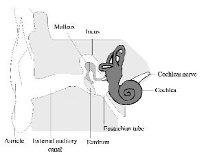
Figure 2.14. Physiology of the ear
The outer ear includes the auricle, whose role is to collect sounds and direct them towards the middle ear via the outer ear canal, which is about 2.5 cm in length. Sounds collected in this way then make the eardrum (a fibrous membrane located at the end of the ear canal) vibrate. Apart from its role as an amplifier, the eardrum plays an important role in the filtering out of certain frequencies and amplitudes.
The middle ear, which is located further in than the eardrum, is made up of a small hollow cavity which contains three ossicles that connect the ear drum with the cochlea. These ossicles include the malleus, the incus and the stapes. The role of these ossicles is the amplification of sound waves and the transmission of these sound waves to the inner ear. This mechanical transmission also ensures that that airwaves are transformed into liquid waves, transmitted via the fenestra ovalis. The difference in terms of the surface between the ear drum and the fenestra ovalis (a factor of 1/25) also contributes to the amplification of sound waves received.
Finally, the inner ear is made up of the cochlea. The cochlea is spiral shaped and has a diameter which progressively contracts. The cochlea is found inside a solid bony labyrinth which is full of fluid. The wave transmitted by the middle ear makes the basilar membrane inside the cochlea vibrate. This allows the initial analysis of sounds to take place, notably in terms of their frequencies, since the cochlea reacts to sound waves in a selective way. The lower part of the cochlea resonates with high-pitched sounds and the upper part (also called the apex) resonates with low-pitched sounds. The selectivity of the cochlea can be explained by the fact that diameter variation implies the existence of a continuum of natural frequencies which allows the cochlea to differentiate a great number of sounds. The hair cells within the cochlea are connected to the cochlear nerve which is made up of approximately 30,000 neuron axons. The movement of these cells triggers a signal which is directed towards the temporal lobe in both hemispheres of the brain. The brain merges these signals and the signal is processed and perceived.
Several perceptual factors influence the way in which we hear sounds, for example, the pitch, the quality of the sound and its length. An average person can perceive sounds with frequencies between 20 and 20,000 Hz. However, most sound frequencies used in natural languages are between 100 and 5,000 Hz. Since frequency variations are not always perceived in the same way by the human ear, we use the term pitch, measured on the mel scale, to describe the perceptual effect of frequencies.
The feeling of pitch, created by voiced sounds, such as vowels and consonants such as [b] and [d], is linked to the frequency of vocal fold vibration, which is also called the fundamental frequency F0. In the case of voiceless sounds such as [s] and [p], the sound produced is the result of the passage of air forced through constrictions. This produces faster pressure variations than with vowels. It is also worth mentioning that pitch variations play an important role in the marking of prosodic differences. When differences in pitch occur in a systematic way within words in certain languages (notably within a syllable) and create differences in the meaning of words as a result, we call these languages tone languages. Examples of such languages include Mandarin Chinese and Vietnamese. When pitch differences occur at the level of the whole phrase, we are talking about intonation, which is a phenomenon that occurs in many languages, including French, English and Arabic.
Volume (or loudness) is the perceptual equivalent of amplitude. Just as with the relationship between pitch and frequency, the relationship between volume and amplitude is not linear, because sounds of a very high frequency or a very low frequency must be of a much higher amplitude to be perceived (compared to sounds with a mid-range frequency). Typically, speaking more loudly is the normal reaction to problems where noise prevents perception. From a linguistic perspective, volume plays a minor role in the study of accents of other prosodic phenomena.
2.1.1.4. The phonetic system of French
Descriptive phonetics considers the global properties of linguistic systems (languages or dialects) as well as comparing them to find universals or phenomena that are specific to a given language. The description is carried out according to articulatory and acoustic criteria. These descriptions are particularly based on the distinction (universally attested in all of the world’s languages) between consonants and vowels.
Vowels are voiced sounds (requiring the vibration of the vocal folds) which come from the passage of air in the oral cavity and/or nasal cavity without or with very little obstruction. To classify vowels, we use features such as manner of articulation, nasality, degree of aperture, as well as backness or frontness, which we will see in detail in the following sections.
The manner of articulation concerns the way in which the speech organs are configured to shape the air that comes from the lungs. This concerns phenomena such as rounding and orality/nasality. Rounding refers to the shape of the lips during the production of a vowel characterized by the pulling in of the corners of the mouth and the lips in the middle. It is accompanied by the protrusion of the lips, creating an additional cavity between the lips and the teeth which some call the labial cavity (see Figure 2.15).

Figure 2.15. Lip rounding
Even though, in theory, all vowels can be pronounced with rounded lips, some can only be pronounced with rounded lips, such as the first group in Table 2.3 [ROA 02].
Table 2.3. Examples of rounded and unrounded vowels in French
| Rounded vowel | Example | Transcription | Unrounded vowel | Transcription | Example |
| [y] | vue | [vy] | [i] | commis | [kɔmi] |
| [œ] | Peur | [pœR] | [e] | nommé | [nɔme] |
| [ø] | Peu | [pø] | [ε] | être | [εtR] |
Nasality is the result of the lowering of the velum, which forces the air to cross the nasal cavity. Since the mouth cannot be closed completely during the production of a vowel, air continues to pass (in parallel) through the oral cavity. In IPA, a tilde is added above the grapheme to mark nasal vowels. Several languages have nasal vowels, such as Portuguese, Polish, Hindi and French, which contains four vowels of this type (see Table 2.4).
Table 2.4. Nasal vowels in French
| Nasal vowel | Examples |
| Mon, tronc | |
| Tente, gant | |
| Brun, défunt | |
| Satin, rien |
French also has a group of 12 oral vowels which are characterized by air only passing through the oral cavity, without nasalization (see Table 2.5).
Table 2.5. Oral vowels in French
| Oral vowel | Examples |
| [i] | Ni, ici |
| [e] | Les, générer |
| [ɛ] | Mes, maison |
| [ø] | Peu, cheveux |
| [y] | Vu, mue |
| [ə] | Le, de |
| [u] | Cou, mou |
| [o] | Bateau, beau |
| [ɔ] | Fort, toc |
| [ɑ] | Pate, mât |
| [a] | Bas, ma |
| [œ] | Peur, sœur |
The degree of aperture is another criterion which allows vowel sounds to be distinguished between one another. It is a question of the distance between the tongue and the palate at a place where the two are at their closest. To find out more about the differences between degrees of aperture, let us look at the following sequence of vowels:
- 1) [i] [y] [u]
- 2) [e] [ø] [o]
- 3) [ɛ] [œ] [ɔ]
- 4) [a] [ɑ]
As we can see, the first series corresponds to three close vowels because the tongue is close to the palate. The second series involves three mid-close vowels, and the third series includes three mid-open vowels. Finally, we have a series of two open vowels where the distance between the tongue and the palate is maximal.
Frontness/backness is an important criterion in the classification of vowels. Front vowels such as [i], [e], [ɛ] and [a] are characterized by the tip of the tongue being at the front of the mouth. On the other hand, back vowels such as [u], [o], [ɔ] and [ɑ] are characterized by the pulling back and bunching up of the body of the tongue (see Figure 2.16).

Figure 2.16. Front vowels and back vowels
Taking the criteria of openness and backness/frontness, we obtain the schematic classification of vowels which takes the form of a trapezium (see Figure 2.17).

Figure 2.17. French vowel trapezium
It is useful to mention that there is a particular vowel in French which is called the silent e. It is transcribed using the [ə] symbol in IPA. This vowel is different to the vowel [ø], which is used in words such as deux [dø] (two). Indeed, both are front rounded vowels in French but with different degrees of rounding, [ø] being more rounded. Phonologically, this vowel has a special status in French because it can appear in precise contexts, notably at the end of a word or before another vowel. Furthermore, geographical considerations can come into play to regulate its pronunciation.
Consonants are sounds that are produced with a closure or a constriction in the oral cavity. In contrast to vowel sounds, the vibration of the vocal folds is not a necessary condition during the production of consonants. However, two main criteria are used to classify consonants: place of articulation and manner of articulation.
The manner of articulation of consonants allows two consonant sounds which share the same place of articulation but which are pronounced in different ways to be distinguished. This allows consonants to be classified according to the following pairs of categories: voiced/voiceless, oral/nasal, plosive/fricative and lateral/vibrant.
Voicing is the property of consonants whose pronunciation involves the vibration of the vocal folds. Thus, we have two series of consonant sounds: series (a) represents voiceless consonants and series (b) represents voiced consonant sounds.
- a) [p] [t] [k] [f] [s] [ʃ]
- b) [b] [d] [g] [v] [z] [ʒ]
In a practical way, to find out whether a consonant is voiced or voiceless, you can put your finger on your throat to feel whether there are vibrations.
As we have seen with vowel sounds, nasalization is a property which is the result of air passing through the nasal cavity due to the lowering of the velum (see Figure 2.18). In French, there are three nasal consonants: [m], [n] and [ɲ], like in gagner (win). To test whether a consonant is nasal or not, you can block the nose while pronouncing this consonant. If the sound changes in quality, this shows that the consonant sound is nasal.

Figure 2.18. Nasal and oral consonants
Some consonant sounds are pronounced in a continuous and homogeneous way (through time), while others are quick, due to the complete closure of the vocal tract and then the sudden escape of air from this point of closure (like an explosion). This property allows fricatives (series a), which are continuous, to be distinguished from plosives (series b), which are quick.
- a) [f] [v] [s] [z] [ʃ] [ʒ]
- b) [p] [b] [t] [d] [k] [g]
From an articulatory point of view, the continuous aspect of fricatives is due to the constriction of the air passing through the vocal tract but without complete closure. Once the speech organs are in place for a fricative, they do not move. This gives fricative sounds a homogeneous character. However, the production of plosives requires the speech organs to move and, therefore, a heterogeneous sound is produced.
A lateral consonant is a consonant whose pronunciation involves air passing down the sides of the tongue. In modern French, there is only one lateral consonant: [l]. Conversely, a vibrating consonant is the result of one or more taps with the tongue tip or the back of the tongue making repeated contact against the uvula. For example, with the [r], which is commonly called apical, the tongue is placed against the upper teeth but produces a tap which allows air to pass through.
For consonant sounds, the place of articulation is the area where two articulators come close or touch one another, forming a partial or full closure of the vocal tract. This allows French consonants that we are taking as an example here to be classified according to Table 2.6:
Table 2.6. Places of articulation of French consonants
| Place of articulation | Phonetic category | Examples |
| Lips | Labial or bilabial | [p], [b], [m] |
| Teeth and lip | Labiodental | [f], [v] |
| Teeth | Dental | [t], [d], [n] |
| Alveolar ridge2 | Alveolar | [s] |
| Palate | Palatal | [ɲ], [ʃ], [ʒ] |
| Velum | Velar | [k], [g] |
| Uvula | Uvular | [ʁ] |
There is a category of sounds that lies between consonant and vowel sounds and these are sometimes called semi-vowels or glides. These in French are non-syllabic vowel sounds (which cannot form the nucleus of a syllable) which, when next to syllabic vowels, form part of a diphthong, while also having linguistic properties which are similar to those of consonants. In some respects, semi-vowels could be defined as fricative consonants, which correspond to particular vowels sharing their place of articulation. The list of semi-vowels for French is given in Table 2.7.
Table 2.7. French semi-vowels
| Semi-vowel | Example | Corresponding vowel |
| [j] | Feuille [fœj] | [i] |
| [ɥ] | Puis [pɥi] | [y] |
| [w] | Bois [bwa] | [u] |
Finally, coarticulation is a phenomenon in phonetics which deserves to be mentioned. It occurs when a given sound influences the pronunciation of another sound or several sounds which follow or precede it. For example, in the case of a sequence of French words such as robe serrée (tight dress), the voiced b is influenced by the voiceless s and becomes a p. The sequence is pronounced [ʁɔpseʁe]. In this case, phoneticians talk about the assimilation of voicing.
2.1.2. Phonology
This is a branch of linguistics which looks at the functioning of sounds in the framework of a language system. In contrast to phonetics, phonology looks at sounds as abstract units and not as concrete physical entities. As a consequence, phonology adopts an abstract basic unit, the phoneme, not the physical sound adopted by phonetics. For a general introduction to phonology from a computational perspective, a good reference is [BIR 03].
2.1.2.1. The concepts of phonemes and allophones
The phoneme is a fundamental unit in phonology. It is the smallest unit in language which does not hold any meaning of its own, but changing one phoneme for another causes a semantic change. For example, the replacement of the phoneme /p/ in the word pit by the phoneme /b/ leads to a clear change in meaning, since the word bit is created. Since the words pit and bit only differ by one phoneme, we call them a minimal pair. These groups of words are particularly useful for identifying phonemes in a language. Sometimes, sound differences do not lead to semantic differences. This is the case notably with dialectal variations of the same phoneme, and the best-known case of this in French is with the phoneme /r/. It is well known that depending on the geographical zone, this phoneme is realized by the sounds [r], [R] and [ʁ]. Therefore, we are talking about three allophones. In other languages, these three sounds, or two of them as, in Arabic, correspond to three distinct phonemes. This demonstrates that two or more sounds can be allophones in one language and distinct phonemes in another.
It must also be outlined that although phonetics and phonology examine different aspects of speech, they share a number of things in common, for example the distinctive features that we will detail later (see [KIN 07] for more information about the connection between phonetics and phonology).
2.1.2.2. Distinctive features
Since the Middle Ages, linguists have recognized that sounds are not simple units but rather complex structures made up of phonetic characteristics. At the beginning of the 20th century, the Russian linguist Nicolaï Troubetzkoy described this aspect of phonemes in terms of oppositions and he identified several types of oppositions [TRO 69]. He described binary oppositions, which imply two phonemes that share properties in common, such as the phonemes /p/, and /f/, and exclusive oppositions, which show that in a pair of phonemes, only one might possess a particular trait (e.g. voicing in the case of /v/ and /f/, where only /v/ is voiced). He also described multilateral oppositions that concern several phonemes such as /p/, /b/, /f/ and /v/. Finally, he broached continuous oppositions which, by their very nature, vary in degrees such as the height of the tongue necessary for the production of a vowel.
The proposal for what is now known as the distinctive feature theory is historically attributed to Roman Jakobson whose work with Gunnar Fant and Morris Halle laid its foundations [JAK 61]. Jakobson’s model stipulates, among other things, that all phonological features are binary. This means that a phoneme either possesses or does not possess a trait of whatever kind, therefore making the discretization of the gradual oppositions described by Troubetzkoy necessary. The advantage of this rule binarization is that it makes the expression of phonological rules much simpler. To guarantee the universality of its description, Jakobson opted for acoustic features, therefore avoiding articulatory features which are too dependent on specific language. The result of his taxonomy is a collection of 12 features: consonantal, compact/diffuse, grave/acute, tense/lax, voiced, nasal, continuant, strident (elevated noise intensity)/non-strident, obstruent, flat and sharp. For example, the phoneme /a/ possesses the following features: +Vowel, −Nasal, +Grave, +Compact.
Reexamined by Noam Chomsky and Morris Halle in their book The Sound Pattern of English (SPE), the concept of the distinctive feature becomes less abstract and gives way to a richer taxonomy. According to the SPE model, features are categorized according to five groups: major features, place of articulation features (cavity), manner of articulation features, source features and prosodic features [CHO 68] (see Table 2.8).
The description of phonemes in terms of features opens the path to generalizations in the form of phonological rules, which give way to the study of a number of morphological phenomena such as joining and assimilation.
Table 2.8. Examples of distinctive features according to the taxonomy by Chomsky and Halle [CHO 68]
| Class | Features | Explanation |
| Major features | Syllabic [+Syll] | This feature indicates that the phoneme is capable of making up a whole syllable by itself. In French, for example, only vowels have this property, but in English, some consonants can be syllabic like the consonant l in bottle. |
| Consonantal [+Cons] | This feature concerns the phonemes whose production involves a major vocal tract obstruction such as plosives, liquids, fricatives and nasals. | |
| Sonorant [+Son] | This feature indicates a significant opening of the vocal tract: vowels, semi-vowels, liquids and nasals. | |
| Place of articulation | Coronal [+Cor] | This feature is connected to consonants where the tip of the tongue gets close to or touches the teeth or alveolar ridge. |
| High [+High] | The body of the tongue rises to get close to or touch the palate. | |
| Anterior [+Ant] | The place of articulation is located at a frontal position in the mouth (alveolar ridge, teeth, lips, etc.). | |
| Back [+Back] | The place of articulation is located with the tongue behind the palatal area. | |
| Manner of articulation of consonants | Sonorant [+Son] | This feature allows vowel and consonant phonemes which require the vocal and nasal tract to be as unconstructed as possible to be grouped together. Liquids and nasals are examples of consonants which have this feature. |
| Continuant [+Cont] | This feature allows sounds whose pronunciation can be prolonged (e.g. fricatives) to be distinguished from phonemes that cannot be prolonged (e.g. plosives). | |
| Nasal [+Nas] | Phonemes whose pronunciation requires free airflow through the nasal cavity. | |
| Manner of articulation of vowels | High/Low [+High]/ [+Low] | This feature indicates the position of the tongue in the mouth, marking the degrees of aperture of the vowels: open [+Low], close [+High]. |
| Back [+Back] | The body of the tongue is pulled back. | |
| Round [+Round] | Phonemes produced with rounded lips. |
2.1.2.3. Phonological rules
This is a formal tool used most notably in the framework of generative phonology to describe a phonological or morphophonological process. The rules can apply to phonetic transcriptions or to feature structures. The modern format of these rules was proposed in the framework of the SPE model. Their general system has the following format: A → B / X_Y. In this system, X represents the position on the left and Y represents the right, while A and B correspond to the entry and exit symbols, respectively. In other words, after applying this rule, the sequence XAY will be replaced by the sequence XBY. To express higher level constraints, it is possible to eventually use the symbols $, +, # and ## to mark the boundary of a syllable, a morpheme, a word or a phrase, respectively. Likewise, the symbol ø, used to mark an empty element, is particularly useful for expressing the suppression of an element in the entry sequence.
To clarify the functioning of these rules, let us examine the following example:

This rule describes the replacement of n by an m in standard Arabic if the final sound is followed by a b, independent of what is found in the left-hand position. For example, the n in the preposition ﻣﻦ [min] (has several English equivalents depending on context including of and from) becomes m when it is followed by the adverb baʕd (after), which begins with a bﺑﻌﺪ ﻣﻦ and the result is the following pronunciation [mimba![]() di] ([ALF 89], see [WAT 02] for similar phenomena in Arabic dialects). It must be noted that a similar change occurs in Spanish but in different conditions, which require the description in terms of distinctive features:
di] ([ALF 89], see [WAT 02] for similar phenomena in Arabic dialects). It must be noted that a similar change occurs in Spanish but in different conditions, which require the description in terms of distinctive features:

Following this rule, the phoneme n becomes m, if it is preceded by a vowel (such as [a], [e], [o], [i] and [u]) and followed by a consonant which is labial and an obstruent like [p], [b] and [f]. Thus, n does not change in a case like [en espaɲa] but it becomes m in cases such as:
- – en Porto Rico [em poɾtoriko], en Paris [em paɾis];
- – en Bolivia [em boliβja], en Barcelona [em baɾθelona];
- – en Francia [em fɾansja].
Phonological rules can occur in many different ways and they can be grouped into four categories: assimilation, dissimilation, insertion and suppression.
Assimilation involves changing the features of a given phoneme to make it phonetically more similar to another phoneme, which is usually adjacent but sometimes further away. The preceding two rules describe a case of consonantal assimilation under the effect of a neighboring consonant. The assimilation of the vowel [ε] in the French verb “aider” (to help) [ɛde] is a good example of vowel assimilation. This vowel is often pronounced [e] under the effect of the final vowel. In this case, since the two vowels are not adjacent, we can say that this is non-contiguous assimilation.
Dissimilation is a phonological phenomenon which has been shown both historically and in today’s languages. In contrast to assimilation, it involves the systematic avoidance of the occurrence of two similar sounds being next to each other [ALD 07]. Let us look at the following examples from a Berber language [BOU 09]:

This gives us the following rule:

Insertion involves adding a sound into a given phonological context. In English, a typical case involves adding the schwa [ə] at the end of words which finish with an s (before an s ending) such as in the word bus [bʌs], which becomes buses [bʌsəz] in the plural. Another example of insertion comes from Egyptians speaking English. The language spoken in Egypt does not allow three consonants to be pronounced in succession. Some Egyptian speakers of English will add a vowel sound to avoid three consonant sounds in succession. The sentence: I don’t know exactly [aɪ doʊnt noʊ ɪɡzæktli] becomes [aɪ doʊnti noʊ ɪɡzæktili] with the insertion of the vowel i at the end of the words don’t and exact.
Suppression can affect a given sound in a precise context where the speaker thinks that it will not cause an ambiguity if it is introduced. A typical case in French is the suppression (by certain speakers) of the schwa [ə] in words such as the verb “devenir” (to become) [dəvəniʀ] which might be pronounced [dvəniʀ] or the adjective “petit” (small), which is pronounced [pti]. Likewise, the last consonant in a word, like the final t in the adjective petit or the s in the determinant les, is not pronounced when it is followed by an obstruent, a liquid or a nasal. On the other hand, this consonant is pronounced when it is followed by a vowel or a semi-vowel. Let us look at the following examples:

This gives the following rule:

In spite of the simplicity of these rules, using them as a representation framework is not unanimously agreed upon within the community, notably due to the ambiguity surrounding the order of their application. Different alternatives have been proposed to resolve this problem. One such alternative, which is the most easily applied in NLP, is two-level phonology. This theory will be the focus of a specific section in this chapter. Other approaches recommend using logic to maximize the rigor of the description framework, therefore minimizing the gap between the theory and its computational implantation [GRA 10, JAR 13].
2.1.2.4. The syllable
The concept of the syllable allows describing phenomena at a higher level than the phoneme level, which is the main focus of the SPE model. It involves an abstract phonological unit which corresponds to an uninterrupted phonetic sequence. As a phonological unit, a syllable can either have meaning or not.
The simplest approach involves characterizing the syllables in a language in a linear way, such as sequences of consonants (C) and vowels (V). Let us take the following as examples: a, V, the CV, cat CVC, happy CV-CV, basket CVC-CVC. As we can see, some syllables end with a vowel and are called open syllables (like CV), while others end with a consonant and are called closed syllables (like CVC).
Other theoretical approaches stipulate that the syllable should have a hierarchical structure [KAY 85, STE 88]. Following these approaches, a syllable (σ) is made up of two main parts: an onset (ω) and a rime (ρ). The onset is universal and present in all the world’s languages. Although some languages allow empty onsets, they nevertheless require a structural marker to show this, often in the form of joining. For example, the syllable y [i] in French has an empty onset which is filled by the joining (liaison) phenomenon, like in “allons-y” (let’s go (there)) [alɔ̃zi]. The rime is an obligatory part in every well-formed syllable. The rime is made up of two elements: the nucleus (v) and the coda (k). The nucleus is the most sonorous part of the syllable and is the underpinning element of the rime. This is why it is considered an obligatory element. In French, the nucleus is made up of a vowel, a diphthong, or both at the same time. However, some languages, including Czech, allow a nasal consonant or a liquid to fulfill this role. The coda is optional and has a descending sonority. It is made up of one or several consonants. Consequently, the syllables that have a coda are also closed syllables. Let us look at some examples in Figure 2.19 to illustrate some syllabic structures in French.

Figure 2.19. Examples of some possible syllabic structures in French
As we can see in Figure 2.19, the onset of the first syllable is the null element (ɸ). This is a way of marking that the onset is obligatory but that in this specific case, it is empty. Likewise, we can see that some constituents can form branches, like the onset in the syllable pra, the onset and the coda of the syllable fRɛsk or the nucleus of the syllable croire.
2.1.2.5. Autosegmental phonology
The SPE model has been criticized for several reasons. One reason is because it emphasizes the rules more than the substance of phonological representations. The other reason is the overgeneration of certain rules which are capable of producing unattested cases in the language whose system they are meant to be describing. This contributed to the emergence of different models including autosegmental phonology, an important extension of generative phonology, which was proposed by John Goldsmith also under the name nonlinear generative phonology [GOL 76, GOL 90] (see [PAR 93, VAN 82, HAY 09] for a general introduction).
This theory is based on abandoning the principle of the strict linearity of language introduced by Saussure in favor of a multidimensional vision of the linguistic sign previously defended by linguists from different branches of the field such as [BLO 48, FIR 48] and [HOC 55]. Thus, according to this theory, phonological representations are made up of several independent tiers, each having a linear structure.
The segmental tier focuses on distinctive features more than phonemes to give a finer granularity to the representation. For example, the phoneme /p/ is represented by the following features: [-sonorant, -continuant, -voiced and -labial]. To overcome the redundancy of the representations of these features, several models have been proposed to take the concept of underspecification between the features into consideration [MES 89, KIP 82, ARC 88, ARC 84].
The timing tier corresponds to the succession of units of time and is used as a pivotal point for the other tiers. It allows complex and long segments to be processed. Typically, these units are noted in the form of a sequence of characters, marked as x in the tree, and are associated with segments. For example, the consonant m which is doubled in the spelling of the French words “emmener” and “emmagasiner” receives two temporal units (see Figure 2.20).

Figure 2.20. Examples of how double consonants are dealt with by the timing tier
The tonal tier contains information which shows the distribution of tones at the level of phonological representation. Several studies have shown that this tier is independent of segments since changes in elements at the segmental level do not affect the tonal structure that these elements carry. Tonal information is particularly important for tone languages such as Vietnamese and Chinese.
The autosegmental tier allows the study of long-distance vowel and nasal harmony [CLE 76]. This phenomenon is well known in certain South American languages, such as Warao which is spoken in Venezuela and Tucano and Barasana, spoken in Colombia. In these languages, nasality spreads from consonants to neighboring vowels like in nãõ +ya → nãõỹã, he is coming [PEN 00] (see Figure 2.21).

Figure 2.21. Propagation of nasality in Warao
The syllabic tier allows the constraints linked to the elements of the syllable that we saw in the section on the syllable (onset, nucleus and coda) in each language to be studied. The information in the syllabic tier corresponds to the root of the tree σ, while the segmental level corresponds to the phonemic sequence. As Paradis [PAR 93] highlights, differences in syllabic structure allow interesting phonological phenomena to be explored, such as joining (liaison) of words, e.g. l’oiseau [wazo] (“bird” in French), where the semi-vowel w is considered to be a part of the nucleus and not the onset, while this joining does not occur in la ouate [wat] (“wadding” in French), since w is part of the onset.
The metrical tier concerns the supra-syllabic level and allows phenomena such as the accentuation of one or more syllables, and other prosodic phenomena, to be described. This includes intonation that we will detail later (to avoid repetition of other prosodic phenomena).
As a theory of the dynamics of phonological representations, autosegmental phonology covers the rules about well-formedness, allowing the association of one tier’s element with an element of another tier.
Autosegmental phonology has seen important developments, notably following McCarthy’s work which promised to generalize the theory to take into account languages with non-concatenative morphology such as standard Arabic [McC 81].
2.1.2.6. Optimality theory
Proposed by Alain Prince and Paul Smolensky, optimality theory (OT) is a linguistic model situated in the framework of generative grammar. It states that the surface structure of languages is the result of the resolution of a certain number of conflicts between several constraints in competition [PRI 93, PRI 04]. The linguistic system is, therefore, considered as a system of conflicting forces. Although phonology is the field that OT fits into best, many works have attempted to apply its principles in other branches of linguistics, such as morphology, syntax and semantics (see [LEG 01, HEN 01, BLU 03]).
In contrast to the SPE model, the OT uses constraints more than rules. For example, in the SPE model, to express the fact that in Egyptian, three consonants cannot appear in succession, rules such as those provided below are used.

In practice, this gives us cases like:

To process this case from the perspective of OT, we need to use the constraints that can be organized in a table (see Table 2.9).
Table 2.9. Constraint forbidding three successive consonants in Egyptian Arabic
| Entrance | *CCC |
| il bint kibiː ra | * |
| il bint – I – kibiː ra |
As we can see in Table 2.9, the constraint of forbidding three successive consonants is violated by the first candidate (marked by an asterisk) and not by the second. This explains why the second candidate, marked by the pointing hand, is preferred over the other. If we take the different constraints implied in the formation of a sentence, we will find a number of candidates in competition and each will obey different constraints (but not all the constraints). The optimal candidate will, therefore, be the one that satisfies the most constraints.
To put candidates in order, OT distinguishes between different types of violations: a violation marked by an asterisk and a crucial violation marked by an exclamation mark. Let us examine the case of joining in French and constraints that are exemplified by two possible candidates [pəti ami] (boyfriend) and [pəti t ami] presented in Table 2.10. The constraints that apply to an example of this kind can be classified into two major categories: markedness constraints and faithfulness constraints. Markedness constraints imply a minimization of markedness and, therefore, cognitive effort, which contributes to a maximization of discrimination. In practice, this is realized by a preference for simple linguistic structures which are commonly used and easy to process. For example, all the languages in the world have oral vowels but few have nasal vowels. Likewise, all the languages in the world have words that begin with consonant sounds but few languages allow words to begin with vowel sounds. Identity constraints put structural changes upon entry at a disadvantage. In other words, they require words to have the same structure on entry as on exit: no insertion, no suppression, no order changes, etc.
As we can see in Table 2.10, we have two constraints which are in competition. Firstly, the constraint that two vowels cannot be next to each other is violated by the second candidate, but not by the first. We can also see that the faithfulness constraint is violated by the first candidate, which involves the insertion of a t. Since the first constraint is very important in French, its violation is considered to be fatal. Thus, the first candidate is favored, even though it violates the faithfulness constraint (see [TRA 00] for a more detailed discussion of similar examples in French).
Table 2.10. Constraints involved in the case of joining (liaison) in French
| Entry | *VV | Faithfulness |
| peti t ami |
* | |
| peti ami | *! |
It can be said that the main advantage of OT is its explanatory ability. In contrast to the rules which must be satisfied by the surface structure, the constraints bring to light factors which might otherwise be hidden (not visible on the surface) but which contribute to the emergence of the optimal output structure.
From a computational point of view, the formal establishment and models of OT implicate other theoretical frameworks, such as autosegmental phonology used by Jason Eisner, who proposed a formalization of OT based on finite-state automata [EIS 97]. Based on Eisner’s model, William Idsardi showed that the problem of OT generation is NP-hard and that it cannot give an account for phenomena of phonological opacity because it does not possess an intermediary level of rules to apply [IDS 06]. The Idsardi test was called into question by Jeffrey Heinz [HEI 09] who argued that it only applies to a particular part of OT. Boersma [BOE 01] proposed a stochastic view of OT where the constraints are associated with a value on a continuous scale rather than on a discrete scale of priority. Other formalization works have emerged in the field of syntax (see [HES 05] for a general review of the applications of OT in computational linguistics). Furthermore, a learning framework for OT was proposed by Bruce Tesar [TES 98, TES 12].
2.1.2.7. Prosody and phono-syntax
Prosody is a term in suprasegmental phonology used to discuss supraphonemic phenomena such as the syllable, intonation, rhythm and flow [CRY 91, BOU 83] (see [VOG 09] for a typological overview). From a phonetic point of view, the parameters which allow prosody to be characterized include height, acoustic intensity and the duration of sounds. These parameters are directly affected by the emotional state of the speaker, which gives prosody an additional dimension.
In the field of NLP, prosody plays an important role in a number of applications, notably speech synthesis, emotion recognition, the processing of extra-grammatical information in oral speech, etc. Given the complexity of interactions between prosody and superior linguistic levels in French, we will concentrate on prosodic phenomena in this language, while also mentioning notable phenomena in other languages.
2.1.2.7.1. Stress
Stress has the function of establishing a contrast between different segments, defined by phonological, syntactic and semantic criteria, which are stressable units. As Garde [GAR 68] underlines, the criteria chosen to define these units vary from one language to another. Consequently, stress has the role of giving a formal marker to a grammatical unit, the word, which is an intermediary between the minimal grammatical unit, the morpheme and the maximal grammatical unit, which is the sentence.
Stress can be marked using two different types of processes: positive and negative. Positive processes involve the increase in intensity of the syllable, which is stressed in comparison with unstressed syllables. Another factor that contributes to a syllable being stressed is prolonging the length of the nucleus of the syllable in question, as well as a noticeable increase in its fundamental frequency. In contrast to positive processes, negative processes involve the removal of a feature in unstressed syllables. Logically, these processes affect the features that belong to the inventory of distinctive features in the language.
In French, stress units have limits which are highly variable and depend on factors such as the succession of syllables which are susceptible to being stressed, the rhythm of speech and pauses. The majority of words are susceptible, in certain positions, to becoming unstressed. In reality, stress does not affect units that can be described based on fixed linguistic criteria. It is more a question of units whose limits vary from one utterance to another. This is how French tends to avoid the immediate juxtaposition of two stresses. Apart from this case, French excludes the possibility of semantically close words all being stressed in near succession unless there are pauses. Groups of words like this become longer and the flow becomes gradually more rapid and less careful. Given that there is no syntactic category that systematically carries the stress in French, it is impossible to syntactically define a stress unit. On the other hand, we can define the syntactic constraints which affect the realization of stress. For example, we know that the stress cannot be placed on an article such as le or la (the), since these morphemes are always integrated into a larger stress unit.
In some languages, the position of the stress, in the framework of a stress unit which has already been set out, depends upon syntactic criteria. These languages are called variable stress languages. In other languages, called fixed stress languages, the position of the stress depends on phonological criteria. In French, stress is fixed, because it falls on the final syllable in the stress unit.
Now, let us consider an important variant of ordinary stress in French which is called insistence stress. Just as with ordinary stress, it is based on the idea of an intentional contrast which allows certain elements of the utterance to become the focus of the utterance. In contrast to ordinary stress, this insistence stress falls on the first syllable of the word in French and this causes perceptibility to increase. In French, it is possible to distinguish two processes in prosodic insistence: emotional insistence stress and intellectual insistence stress [GAR 68]. Emotional insistence stress involves prolonging the first consonant of a word with an emotional value or pronounced with disapproval, like in C’est formidable (it’s wonderful) or C’est épouvantable (it’s terrible). Intellectual insistence stress involves reinforcing intensity by increasing the fundamental frequency as well as lengthening the first syllable of the stressed phrase [GAR 68]. It is mainly used to mark the opposition between two terms like in c’est un chirurgien qui a opéré le patient, pas un infirmier (it was a surgeon who operated on the patient, not a nurse) or in the following exchange:
- – Un billet d’avion avec une chambre d’hôtel ? (A plane ticket with a hotel room?)
- – Non, un billet d’avion seulement. (No, just a plane ticket)
The position of the intellectual insistence stress is not always the same as in the case of emotional insistence stress. Both are on the initial syllable when the word begins with a consonant. On the other hand, in words which begin with a vowel sound, intellectual insistence falls on the first syllable and emotional insistence falls on the second.
2.1.2.7.2. Intonation
Intonation, in the broadest sense of the term, covers a whole series of physical parameters which vary with time, such as intensity, fundamental frequency and silence. Psychoacoustic parameters also come into play with intonation. Stress, melody, rhythm, prominence, breaks, etc. are all important [ROS 81, ROS 00, GUS 07].
Since the beginning of linguistics, there have been a number of studies investigating the relationships between syntax and intonation, given the possible range of effects of syntax on the surface structure of the phrase. Intonation plays a role in the initial resolution of syntactic ambiguities and, therefore, allows the speaker to choose a particular analysis over other analyses or interpretations. Let us examine the following sentence: John talked #1 about his adventure #2 with Tracy. Depending on the place of the pause (1 or 2), one possible interpretation is preferred. The possible interpretations are as follows, respectively: Tracy went on the adventure with John, or Tracy is John’s conversation partner. Here is another interesting example: John didn’t leave his house # because he was ill. With a pause after the prepositional phrase, the interpretation of this sentence is: John is at home. Without the pause, the interpretation becomes: John is no longer at home but the reason for his having left the house is not the illness. Finally, it is well known that intonation plays an important role in the marking of discursive structures and thematic roles [HIR 84] (see [HIR 98] for a typological review).
2.2. Speech processing
Speech processing (SP) is a term which refers to a variety of applications. Some applications are limited to the level of the speech signal, whereas others rely on high-level linguistic information. In this section, we will focus on the two applications which fit into NLP the best: speech recognition and speech synthesis. Given the nature and the objectives of this book, we will not elaborate on the aspects linked to the processing of the signal itself, but, nevertheless, we will include references for those who would like to know more.
Before going any further, we must quickly present two other applications which are of interest in many respects: speaker recognition and language identification.
Speaker recognition involves identifying the person who utters a phonic sequence whose length varies from long to very short. Such applications require vocal characteristics (which are unique to each and every one of us) to be modeled. To limit the quantity of speech required for training, a generic model is created and the specific models for each speaker are derived from this. Once the models have been created, the process of identification involves measuring the distance between the short sequence produced by the speaker and the existing models. The speaker is identified if the distance between the sample and the model exceeds the pre-established confidence threshold (see [BON 03, KIN 10] for an introduction).
Another application of SP involves identifying the language or dialect of the speaker. From a practical point of view, such applications allow telephone calls to be connected to speakers who are able to understand and interact with the language used, in an international context. However, applications to the field of security remain the most common for this type of systems. The principle of these systems is similar to the systems of speaker identification. This involves creating an acoustic profile for each target language and/or dialect and measuring the distance between the sample received and each of the existing profiles (see [MON 09] for an example of these works).
2.2.1. Automatic speech recognition
Automatic speech recognition (ASR) involves identifying sequences of words which correspond to the speech signal captured by a microphone (see [JUN 96, YU 14] for a general review). The most obvious use for ASR is in the context of human–machine spoken dialogue applications, where data are introduced by means of spoken utterances. Nevertheless, vocal dictation is the oldest and most widespread application of ASR.
To classify ASR systems, several parameters come into play, including the size of the vocabulary and the number of speakers. Table 2.11 presents the main parameters as well as the main characteristics of the systems [ZUE 97].
Table 2.11. Classification parameters of speech recognition systems
| Parameter | Possibilities |
| Speaking mode | Isolated words, continuous speech |
| Speaking style | Read text, spontaneous speech |
| Enrollment | Dependent or independent speaker |
| Vocabulary size | Between 20 and tens of thousands of words |
| Type of language model | Finite state machine or context-dependent |
| Perplexity | Between < 10 (small) and >100 (large) |
Given the complexity of their task, ASR systems have to overcome big challenges. These challenges have given way to highly desirable characteristics, which are:
- – robustness: an ASR system must adapt to different levels of sound quality, including sounds of a poor quality. This poorness of quality can be the result of noise in the environment. This is especially the case in applications that are designed to be used in a car or in an airplane (e.g. the noise caused by the engine or the air). Conversations happening nearby can also present a similar form of challenge;
- – portability: given the cost of the development of an ASR application, it is highly desirable to be able to apply the same work to several areas of the application without much effort being required;
- – adaptability: a good system should be able to adapt to speaker changes and microphone changes and this should be the case whenever it is used. Spontaneous speech comes with its own major challenges to overcome, as it contains hesitations and repetitions which are difficult to model, even with the use of statistical approaches. Finally, a recognition system must be capable of recognizing or at least reducing the impact of the words pronounced which are not already included in its vocabulary.
Typically, a speech recognition system is made up of several modules and each one is specialized, allowing it to deal with a particular aspect of the analysis of the speech signal (see Figure 2.22).
Firstly, the feature extraction module allows features which are useful for the digital and sampled signal to be extracted. In telephone applications, for example, this sampling is carried out at a rate of approximately 8,000 samples per second. In some cases, this module has the role of improving the quality of the signal, by reducing the sources of sound which come from a neighboring conversation, from noise in the environment, etc. This filtering allows the recognition module to be activated intelligently when it is established that the signal received is effectively a speech signal and not noise. For more information on the extraction of features and signal processing in general, refer to [CAL 89, OGU 14] and [THA 14].

Figure 2.22. General architecture of speech recognition systems
Next, the decoding module tries to find the most likely word using acoustic models and language models.
The acoustic model allows hypotheses about words to be generated with the help of techniques such as hidden Markov models (HMM), neural networks, Gaussian models or other models. The result of the acoustic model is a graph of words which sometimes involves a great number of sequences, and each one corresponds to a path in the graph. To identify the best sequence of words in the graph, the decoding module uses a language model which is usually based on n-grams. Note that in spite of the domination of statistical models since the 1970s, different forms of pairing with linguistic models have nevertheless been experimented with.
2.2.1.1. Acoustic models based on HMM
When work first began on ASR, rule-based expert systems were used to detect phonemes. Given the limits of their efficiency and the difficulties surrounding their development, these approaches were abandoned in favor of statistical methods, notably Markov chains. Markov chains are mathematical systems proposed by the Russian mathematician Andrei Markov at the beginning of the last century to model temporal series. The model was then further developed by the American mathematician Leonard E. Baum and his collaborators whose work gave way to the HMMs. The first implementations of HMM in the area of speech recognition took place during the 1970s by Baker at Carnegie Mellon University, as well as Jelinek and his colleagues at IBM [BAK 75a, BAK 75b, JEL 76].
The fundamental idea of Markov chains is to examine a sequence of random variables which are independent of each other. The purpose of such a sequence is that it allows us, through observing past variables, to predict the value of these variables in the future. For example, if we know the monthly rainfall in a given town, we can predict, with a certain margin of error, what the rainfall will be in the subsequent month(s). Therefore, we are talking about conditional probability, where the value of a given variable (quantity of rain predicted for the subsequent month) depends upon the values of variables in the sequence that precedes it (known history of rain in the town in question).
For an introduction to the fundamental concepts of probability, since this goes beyond the objectives of this text, we recommend [KRE 97] and [MAN 99] (for an introduction to these concepts in the context of NLP). A great range of books and manuals giving an introduction to probability exists and, of course, these can be used if necessary.
Let us take a detailed example to explain the principle of the Markovian process (see [RAB 89, FOS 98] for a similar example on climate). Suppose that a given person or robot, whom we will call Xavier, can be in three possible moods: happy, neutral and sad. Suppose also that our Xavier remains in the same mood for the whole day. Therefore, to predict Xavier’s mood tomorrow, it is necessary to know what his mood is today, what it was like yesterday and what it was like the day before yesterday, etc. More formally, we must calculate the probability of p(en+1|en, en-1, … e1). In practice, it is best to take into account a part of Xavier’s mood history with only a limited number of preceding moods. Here, we are talking about a first-order Markov chain (with only one preceding mood) or a second-order Markov chain (with two moods preceding the current mood), etc.
Suppose that we have a chain of random variables X = {X1, X2, .., XT} and each one takes a value v based on a limited range of values V={v1, v2, .., vn}. This gives us the following equations:

The probability of a Markov chain can be calculated according to equation [2.1].
Let us imagine that in the case of Xavier’s moods, we have the probabilities presented in Table 2.12.
Table 2.12. Probabilities of Xavier’s moods tomorrow, with the knowledge of his mood today
| Mood today | Mood tomorrow | ||
| Happy | Neutral | Sad | |
| Happy | 0.70 | 0.27 | 0.03 |
| Neutral | 0.40 | 0.35 | 0.25 |
| Sad | 0.12 | 0.23 | 0.65 |
Table 2.12 shows that the probability of a radical change in Xavier’s mood (e.g. happy→ sad) is generally inferior to that of a gradual change (e.g. happy→ neutral) or to no change at all (e.g. happy→ happy). The information given in this table can be represented in the form of a Markovian graph made up of a finite number of states (which is three in our case – namely neutral, happy and sad), of transitions between these states (arrows or curves) which allow a transition between one state (mood) and another, as well as the probability of staying in the same state (Figure 2.23).

Figure 2.23. Markovian model of Xavier’s moods
This model allows us, for example, to calculate the probability that Xavier’s mood will be neutral tomorrow and happy the day after tomorrow, knowing that his mood is neutral today. This is carried out in the following way:

The idea of Markov chains was pushed even further following the work by Baum and his collaborators who added an additional element of complexity to the model, which is latent or hidden variables, and this gave way to what we today call the hidden Markov models or HMMs. The main purpose of HMMs compared to ordinary Markov chains is that they allow sequences to be dealt with even if they contain ambiguity and, as a consequence, they can be processed in more than one way.
If we come back to our example, we know that in reality it is very difficult to guess if someone is in a good mood or not (hidden variable). The only way of telling this is to observe the person’s behavior (observable variable). We can simplify this into two possible behaviors: smiling or frowning. This allows us to imagine the probability presented in Table 2.13 containing information about whether Xavier is likely to be smiling or frowning, knowing his mood.
Table 2.13. Probability of Xavier’s behavior, knowing his mood
| Mood | Probability of smiling | Probability of frowning |
| Happy | 0.88 | 0.12 |
| Sad | 0.55 | 0.45 |
| Neutral | 0.65 | 0.35 |
A more detailed version of the Markov chain graph (Figure 2.23) with behavioral probability gives the HMM diagram shown in Figure 2.24.

Figure 2.24. HMM diagram of Xavier’s behavior and his moods
As Figure 2.24 shows, the HMM model is based on two types of probabilities: the probability of transition and the probability of emission. Transition relates to the movement from one state to another while emission involves emitting an observable variable based on a certain state.
From a formal point of view, HMMs can be seen as a quintuplet:

If we come back to our example, the HMM allows us to calculate the probability of Xavier’s mood, which can be observed directly, based on his behavior, which is also observable directly. In other words, it is possible to calculate a particular mood ei∈{happy, sad, neutral} based on an observed behavior oi∈{smiling, frowning}. This is carried out with the help of the Bayes formula, given in equation [2.2]:

In practice, we are sometimes more interested in the probability of a sequence of events than the probability of a single event. Thus, for a sequence of n days, we will have a sequence of moods E={e1, e2, …, en} and a corresponding sequence of observable behaviors O={o1, o2, …, on}:

When applied to the problem of ASR, the sequence of acoustic parameters extracted from the speech signal can be described by a HMM. This involves combining two statistical processes: a Markov chain which models the temporal variations, and an observed sequence which allows spectral variations to be examined. The most intuitive way of representing a phonemic sequence is to consider that each state corresponds to a phoneme. Let us examine the example of the French word ouvre (to open) [uvʀ], which is made up of three phonemes, shown in Figure 2.25.

Figure 2.25. Markov chain for the word “ouvre” (open)
As we can see in Figure 2.25, there are two types of transitions between phonemes: a transition between a phoneme and the following phoneme and a cyclical transition towards the same phoneme which allows important variations between the length realizations of each phoneme to be studied. These variations are generally due to the nature of the phoneme (notably continuous vowels and consonants), the differences in the context of phonetic realization, intraspeaker variation or interspeaker variation, etc. Of course, this model is highly simplified because the system in this case can recognize only one word. In applications that are slightly more complex, we have a limited number of words to recognize, like with vocal command systems, where we can give a limited number of orders to a robot or some kind of automatic system. For example, the Markov chain used for the recognition of three (French) vocal commands, namely ouvre (open), ferme (close) and démarre (begin) can have the form shown in Figure 2.26.

Figure 2.26. Markov chain for the recognition of vocal commands
In continuous speech recognition systems with a large vocabulary, a more narrow representation of phonemes is indispensable. Thus, we use several states to represent phonemes. This allows acoustic variations of the same phoneme within a spectrogram to be studied (see Figure 2.27).
Neural networks are a possible alternative for the classification of phonemes (see [HAT 99] for a review). In spite of their results, which are comparable to those of HMM, this technique suffered from significant limitations such as the fact that the learning process is quite slow and that it is difficult to estimate its parameters. Following recent developments in the field of deep learning, which found the solution to these limitations [HIN 06, HIN 12], we are seeing neural networks grow stronger as a real alternative to HMMs.

Figure 2.27. HMM for the word “ouvre” (open)
2.2.1.2. The Viterbi algorithm
As we have said, the role of HMMs in an ASR system is to help find the most likely sequence of phonemes, knowing the acoustic parameters extracted from the speech signal. This comes back to finding the most likely sequence of states or phonemes E = {e1, e2, …, en}, knowing the acoustic parameters observed O = {o1, o2, …, om} and a model λ. In other words, what we are looking for is: p(O, E| λ), which can be calculated using Bayes’ equation (equation [2.4]).
Likewise, the probability of an observed sequence O knowing the HMM model λ can be calculated by the following equation:
To find the most likely path, knowing an observed sequence in a trellis, the easiest solution, but the least efficient, involves calculating the probabilities of every path that allows the sequence in question to be generated, and to then choose the most likely path. A brute force approach like this collides with the size of the research space where the number of possible sequences exponentially increases in the following way: |E|n, where |E| is the number of hidden states in our HMM model and n the size of the entry sequence. In real applications, where the number of states can exceed 100 and the number of words to be recognized can easily exceed 10, we can imagine that the number of possibilities to consider can quickly become impossible to deal with in this way.
The most popular approach for calculating the most probable path is to use the Viterbi algorithm. This algorithm, proposed at the end of the 1960s by Andrew Viterbi, the Italian American engineer [VIT 67], is based on dynamic programming. This paradigm involves dividing the original problem into sub-problems whose solution leads to the solution of the whole problem. The algorithm uses two variables:
– δt(i) is the path for which the likelihood is maximal among all possible paths and ends with the state si at time t:

– ψt(i) allows to store the best path, ending in state si at time t:

The principle of the Viterbi algorithm involves finding the most probable path for each intermediary state and later using it to find the final state in the trellis. Thus, at each time t, we come back to the most probable curve which leads to si. The algorithm is made up of four steps:
1) Initialization:
| δ1(i) = πi. bi,o1, i = 1, .., Ts | where Ts is the number of states and πi the probability of being between a state ei at moment t=1. |
| ψ1(i) = 0 | No state precedes the initial state. |
2) Recursion:
The recursive function is the true heart of the algorithm. Informally, the problem of the final path is cut up into sub-problems whose partial solution is stored in variable ψt for the current state j:

3) Stop condition:
The algorithm stops once we arrive at the final state T:
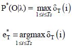
Next, we look for the best path when the end of the observation sequence has been reached at moment t = T, starting with the best vectors ψt.
4) Path backtracking:

To illustrate the functioning of this algorithm, let us go back to the example of Xavier’s behavior. Suppose that we want to calculate the most probable sequence of states, knowing that we have observed the following sequence of behaviors: O = {smiling, smiling, frowning}. Since we do not know Xavier’s initial mood: t0, we will assume that the three possibilities are equally probable. To simplify the presentation, we will adopt the following conventions: Happy = ha, Sad = sa, Neutral = nt, Smiling = sm and Frowning = fr.
1) Initialization:


2) Recursion:
We then calculate the likelihood of being in a certain state based on three possible predecessors, from which we choose the most likely.


At this stage, as Figure 2.28 shows, we have a trellis that is fully populated with three possible paths which contain values of variable ψ as follows:

Thus, the first path is: {happy, happy, happy}, the second is: {happy, happy, neutral} and the final one is: {sad, neutral, sad}.

Figure 2.28. Trellis with three possible paths
3) Stop condition:
We begin to look for the most probable sequence based on the previous stage:

This means that the most probable state with t=3 is neutral.
4) Backtracking:
Based on the previous state found in the preceding stage, we return backwards to the previous state: t = T-1 = 3-1= 2.
Again, we come back to a state: t = T-1 = 2-1= 1.
This means that, knowing the sequence of behaviors observed: O= {smiling, smiling, frowning}, the most likely sequence is E= {happy, happy, neutral}. Note that with the probabilities of transitioning between states only, the most likely path would be {happy, happy, happy}.
2.2.1.3. Language models based on n-grams
After the phoneme recognition phase, ASR systems must find words that correspond to the sequence of phonemes obtained in the preceding phase. Of course, a sequence of letters can correspond to a multitude of possible word sequences. This is due to several factors, such as homophony (two different words with the same pronunciation) or phoneme recognition errors, etc. For example, the (French) phonetic sequence [vjɔlɔ̃sεlki] can correspond to “violoncelle qui” (cello that) as well as “violons celle qui” (violate that one). In the same way, in English, based on the phonetic sequence [naɪ.treɪt], it is possible to obtain two different word sequences: “night rate” and “nitrate”. Furthermore, it must be indicated that language models are used in several applications outside of ASR such as machine translation, information retrieval, text classification, etc.
To find the optimal sequence of words, knowing the sequence of phonemes, several sources of information come into play, notably morphology and syntax. Traditionally, syntactic grammars were used to refine the search for a word sequence. That was abandoned in favor of more statistical approaches sometimes combined with certain forms of syntax [JEL 99]. However, the ideal combination of discrete syntactic knowledge with statistical knowledge, or other forms of continuous knowledge, is yet to be found as much at the level of linguistic theory as at the application level.
From a formal point of view, the probability of observing a sequence of words p(w1, …, wm) is approximated according to the following equation:

The idea of n-grams is to consider the n-1 preceding words rather than the complete history. The hypothesis is that partial information loss is justified by the gain from the reduction in the quantity of linguistic data necessary for n-gram learning. The size of the data required for learning increases with the value of n. The general case of n-grams can be calculated using the following equation:

To fully understand n-grams, we are going to use the following micro-corpus where sentences begin and end with the markers <p> and </p>, respectively:
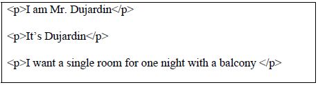
Several types of n-grams exist following the size of the history that is taken into consideration. Unigrams are the simplest form of n-grams. It is a matter of counting the frequency of words out of context in a given corpus, without taking past frequencies into account. However, the raw information from the frequency of a given word in a corpus is difficult to interpret, hence the use of normalization in the form of probability. Thus, we proceed to the division of the frequency of the word in question by the total number of words in the corpus (equation [2.8]):
where C is the number of words in the corpus and f(wx) is the frequency of the word wx. If we begin to count the words in our micro-corpus, we obtain Table 2.14.
Table 2.14. Micro-corpus unigrams
| Word | f(wx) | P(wx) | Word | f(wx) | P(wx) |
| I | 2 | 0.11 | a | 2 | 0.11 |
| am | 1 | 0.05 | room | 1 | 0.05 |
| Mr | 1 | 0.05 | single | 1 | 0.05 |
| Dujardin | 2 | 0.11 | for | 1 | 0.05 |
| it | 1 | 0.05 | night | 1 | 0.05 |
| is | 1 | 0.05 | with | 1 | 0.05 |
| want | 1 | 0.05 | balcony | 1 | 0.05 |
Bigrams involve considering a given word with a back window of a single word. Thus, we are researching different possibilities of occurrences of pairs of words, that is: f(wx wy). Let us take the example of the bigrams of our micro-corpus presented in Table 2.15. It is necessary to add n-1 artificial symbols (hashtags for example) at the beginning and at the end of each sentence to indicate the symbols which are located at the head and tail of the sentence. In the bigram example, the markers <p> and </p> played this role.
Table 2.15. Bigrams in the micro-corpus with their frequencies
| Bigram | f(wx wy) | Bigram | f(wx wy) |
| <p> I | 2 | single room | 1 |
| I am | 1 | room for | 1 |
| am Mr | 1 | for a | 1 |
| Mr Dujardin | 1 | a night | 1 |
| Dujardin </p> | 2 | night with | 1 |
| <p> It’s3 | 1 | with a | 1 |
| It’s Dujardin | 1 | a balcony | 1 |
| want a | 1 | balcony </p> | 1 |
| a room | 1 |
To normalize the bigrams, we can use the following equation:

Based on Table 2.15, we can calculate the probabilities of certain bigrams as follows:

To calculate the probability of the sequence It’s Dujardin, we can proceed as follows: p(<p> It’s Dujardin </p>) = p(It’s|<p>) p(Dujardin|It’s) p(</p>|Dujardin) = 1/3 * 1/1 * 2/3 = 0.217.
Finally, since it is not realistic to assume that the training corpus includes all possible words from the language in question, it is highly recommended to create in advance a specific category for unknown words.
2.2.2. Speech synthesis
A speech synthesis (SS) system is a software or hardware capable of producing speech in an artificial way [TAY 09]. In some cases, the input for such systems can be a phonetic transcription of the entry text or a text annotated with syntactic or prosodic information. However, since the typical input into these systems is a flat text, they are sometimes called Text To Speech systems.
Science historians have reported several attempts to create mechanical machines equipped with spoken functionalities such as Wolfgang von Kempelen’s machine, which was created towards the end of the 18th century. However, the first SS system in the modern sense of the term was probably the VOCODER system, which was developed towards the end of the 1930s at the Bell laboratory in the United States.
From an application point of view, SS systems can be used as independent applications or as modules in larger systems. Applications for the visually impaired or the blind as well as for people with speech disorders are probably the most obvious medical use of such systems. Likewise, human–machine dialog systems use SS modules as a way of interacting with humans. Furthermore, with the increased popularization of intelligent tutoring systems, notably in the field of foreign language teaching, the use of an SS module gives a voice to virtual tutors, allowing them to teach the language in its spoken form. Another important development is the emergence of talking heads or animated virtual characters. There must be a detailed synchronization between the SS and the module that creates the animation of facial and body expressions to guarantee a minimal level of coherence. Of course, the success of all applications depends on the quality and expressiveness of the SS module.
A typical example of the architecture of an SS system is shown in Figure 2.29. Of course, it is more of a general example since the real implementations of modules as well as their modes of interaction can change.
As Figure 2.29 shows, in general an SS system involves two major steps: front-end processing, whose function is to prepare the entry text for synthesis, and back-end processing, which relates to the synthesis of the digital signal. This is done according to several approaches, like concatenative synthesis, formant synthesis and articulatory synthesis.

Figure 2.29. Typical architecture of an SS system
2.2.2.1. Front-end processing
This phase is made up of several stages of low-level linguistic processing, and the majority of these are explained in the following chapters. The first step is the normalization phase, which involves translating written conventions and abbreviations in an explicit format. Let us examine the examples from Table 2.16. As we can see, normalization is far from being a trivial operation. A simple syntactic conversion from one format to another is not enough, but it is clear that we need to access the meaning of the expression to translate it correctly.
The annotation of words by POS tagging (e.g. verb, noun, adjective, etc.), which we will see in detail in Chapter 3, allows certain pronunciation problems linked to homographs of different morphological categories. A typical example in English would be live whose pronunciation as a verb is clearly different from its pronunciation as a noun. In French, the three words couvent, violent and relations for example, can all be nouns or verbs with a different pronunciation for each category. For instance, in the case of couvent (convent (N) or brood (V)), the POS analysis allows the verb (pronounced [kuv]) to be differentiated from the noun, which is pronounced [kuvɑ̃]. However, this annotation does not resolve cases where homographs appear in the same grammatical category. The noun bass is a typical case in English as it may have two different pronunciations ([bas] and [beys]) depending on its meaning. As an example in French we have the word fils (son) [fis] and fils (threads) [fil].
Table 2.16. Abbreviations to be normalized before synthesis
| Abbreviated form | Longer form |
| €1.25 | one euro twenty five |
| 3/5 | three fifths |
| 1/2 L milk | half a liter of milk |
| Sandy is 5 ft. 11 in Sandy is 5’ 11” | Sandy is five feet and eleven inches tall |
| 1 h 30, 1.30 h | one hour and a half or one hour thirty |
| Washington Ave. Delaware Cir. | Washington Avenue Delaware Circle |
Named-entity recognition allows chains of words used to designate a specific object to be detected. It can act upon the title of a book or a film, the name of an institution, a company, a town, etc. Although according to the normative grammar of language such objects should be placed between quotation marks, in practice, many people do not follow this rule, and this makes it necessary to detect entities by non-orthographic means. Let us examine the following examples:
| I saw Gone with the Wind last night. | Title of a film. |
| I would like to see Les Intouchables again with my school friends. | Film title in French. |
As we can see from the above examples, the pronunciation of a named entity must be differentiated from the rest of the sentence to guarantee that it will be considered as such and not as a part of the sentence, in which case it would change the meaning. In cases where the name of the entity is in another language, a special form of treatment is preferred. For example, the proper noun (of Arabic origin) Hamza is pronounced [amza] in English, while in Arabic, it is pronounced [ħamza].
To find the sequence of phonemes based on words, we have the choice between two approaches: a symbolic rule-based approach (written manually or created automatically based on a corpus) and a dictionary-based approach.
The rule-based approach has the advantage of being able to process general cases without a need to store in the computer memory all possible forms. For example, the conversion rules of the grapheme c into s or k can be expressed as follows:
| c → s / ___ {e, i, y} | c is transcribed as s if it is followed by one of the following French vowels: e, i, y. |
| c → k | c is transcribed as k in all other cases. |
Another typical example in French is the pronunciation of the letter g which has two equivalents: [g] and [j] (see [BOS 97, MAN 00] for examples of learning-based approaches).
In the dictionary-based approach, all known possibilities are stored in a database. The advantage of this approach is that it allows the numerous pronunciation exceptions (notably in languages where pronunciation is not very regular, such as English) to be taken into consideration. The CMU pronouncing dictionary, which is freely available on the Internet, is a good example of one of these dictionaries4. It is an electronic dictionary for North American English with 125,000 words transcribed phonetically (stress marks included). The transcription format adopts the Arpabet code and includes 39 phonemes. The vowels are annotated with a number which indicates the stress that they carry. Thus, 0 indicates that there is no stress, 1 indicates a primary stress and 2 indicates a weak secondary stress which tends to be used in compound words such as Vacuum Cleaner, for example. Some transcription examples are given in Table 2.17.
Table 2.17. Examples of transcriptions with the Arpabet format
| Phoneme | Word | Transcription without stress marks | Transcription with stress marks |
| AA | odd | AA D | AA1 D |
| AE | at | AE T | AE1 T |
| AH | hut | HH AH T | HH AH1 T |
| IH | it | IH T | IH1 T |
The problem is that a dictionary, whatever its size, is limited and cannot cover all the words in a language, especially neologisms. To limit non-covert cases in the dictionary, some researchers proceed to the concatenation of compound words or morphemes. For example, imagine that we have to process the word bavardation, which is not listed in a French dictionary. We could assume that we are looking at a case of concatenating the French root bavard (chatty) and the suffix ation. Likewise, the English neologism boatness can be the result of the concatenation of the word boat with the suffix ness.
Finally, based on the above information, the prosodic analysis module allows the text to be analyzed to detect the units which are capable of receiving prosodic forms. The expression of emotions is an important subject, which is directly linked to prosody. The same utterance pronounced with different stress patterns leads to different emotional charges being attached, and this can sometimes change the meaning of the utterance (see [BUR 15] for a review of this work).
2.2.2.2. Concatenative synthesis
Concatenative synthesis is the most intuitive method because it involves putting recorded sequences of speech end to end. Besides its simplicity, it has the advantage of producing a good quality of speech, even though the passage from one sequence to another sometimes causes audible noise. The question which is posed here is one of optimal granularity. Of course, it is tempting to record relatively long sequences of speech such as entire sentences. Such units are well adapted for applications which do not require a large amount of variation in the message, such as indicating the next subway stop. In this case, in a simplified context, it is possible to imagine that it is sufficient to record a station announcement sequence (and the sequence of station names) like in the following example:

etc.
Since the majority of applications require much larger variations in terms of messages, an extreme case being the synthesis of open texts, we must think about using more fine-grained units. The other extreme, in terms of granularity, involves recording the phonemes and concatenating them. Although this approach seems to respond to the need for message variability, it does not consider contextual phonetic variations caused by coarticulation, and therefore, considerably reduces the quality and the intelligibility of the speech.
To take coarticulation into consideration at a local level, larger units are used such as diphones, triphones or nphones, for general cases. Some researchers, like Thierry Dutoit, call this method segmental unit selection speech synthesis [DUT 00]. A diphone is an acoustic segment which begins at the center of the stable zone of a phoneme and ends at the center of the stable zone of the next phoneme. In the case of non-continuous phonemes, it is possible to take the most stable part or simply use triphones [DUT 97]. If the number of phonemes in a given language is equal to N, the number of diphones in this language is theoretically equal to N2. Since not all theoretical combinations are authorized by linguistic systems, the real number of diphones is much smaller. For example, the 25 phonemes of Japanese give way to 625 diphones and the 40 phonemes of English produce 1,600 diphones but in both languages, only one part of the possible diphones is practically usable [BLA 00].

Figure 2.30. General architecture of a concatenation synthesis system
As Figure 2.30 shows, the first step in the process of constructing a SS system consists of collecting linguistic data in the form of a speech database, which must be representative of all the diphones of the target language. The simple approach involves retaining only the example of diphones which is judged to be the most representative. These sequences include all possible combinations of consonants, vowels and silence, which can be considered as a phoneme in the model. A more elaborate approach involves storing several examples of diphones with different prosodic properties, notably in terms of pitch and duration. This allows prosodic processing to be reduced to a minimum The cost of this reduction to increase of the size of the database.
Next, the signal retained for the base is edited and segmented with the help of specialized software, the most common one being Praat, developed by Dutch phoneticians Paul Boersma and David Weenink5. To facilitate adding prosodic parameters and to reduce the size of the database, it is necessary to carry out signal sampling with a method like linear predictive coding. Among the most popular systems developed with this technique, we can cite the MBrolla system from the Mons Polytechnic in Belgium as well as the Festival system developed at the University of Edinburgh in the UK and Carnegie Mellon University in the United States [DUT 96, LEN 00].
To guarantee the best quality of synthesis, industrial approaches adopt more varied natural units, which are generally superior to diphones, such as phonemes, syllables or morphemes. On the one hand, it allows the coverage of coarticulation phenomena on a broader scale. On the other hand, it also reduces the acoustic and prosodic treatments, thus guaranteeing better quality speech production. To find these stored units in an efficient way, an index is created with information such as acoustic characteristics, duration or the phonemic context of each unit.
The main downside of this method is the large quantity of speech that needs to be recorded, which can be up to several dozen hours.
2.2.2.3. Formant synthesis
In contrast to concatenation synthesis, this approach does not require a data sample to be stored because speech is produced in an entirely artificial way, based on an acoustic specification of the first formants of the sound [KLA 80]. Each formant is typically described using three acoustic parameters, namely frequency, amplitude and bandwidth, which represent the breadth of the spectrum signal surrounding the formant. In the majority of approaches, the oral and nasal cavities are modeled in a parallel way and then combined with a propagation module which simulates the nose and the lips. This particular method is not interested in modeling the speech production process by humans, but rather in modeling its entry and exit. In other words, the human phonatory system is considered a black box.
In a general way, this approach uses the source–filter model where the source models the activity of the vocal folds and the filter represents the vocal tract, which produces the formants. The sound source for vowels and consonants can take different forms according to their phonetic characteristics. Thus, the source for vowels and voiced consonants is either a periodic function or the output of a linear time-invariant filter, which takes a sequence of impulses as its input. Sounds implying an obstruction are generated based on random noise (white noise), while voiced fricatives use two sources. Formants are then created based on a second-order filter, which reduces the high frequencies and the amplitude from their source. Two types of architectures are possible: serial architecture and parallel architecture (see Figure 2.31). Serial architecture requires the frequency and the bandwidth of each resonance, as well as the common gain. This architecture, which is capable of approximating oral sounds, presents limits when it comes to approximating nasal sounds or fricative sounds. Parallel architecture is capable of approximating any kind of speech spectrum but requires the individual gains at the input of each filter.

Figure 2.31. Serial and parallel architecture of formant speech synthesis systems
This technique offers multiple notable advantages. Apart from the good intelligibility of the speech that it produces, it allows the memory necessary for the system to be reduced, as it does not store speech. Furthermore, since speech is produced in a completely artificial way, it gives a very high level of control to parameters such as prosody and flow. The only disadvantage is probably that speech synthesized using this method can be quite robotic in some cases.
2.2.2.4. Articulatory synthesis
Articulatory synthesis is a technique which is based on the computational modeling of the physiological process of speech production. According to this approach, the sound produced is the result of the interaction of the vocal source with a filter that corresponds to one or several speech organs (see [PAL 06] for a general review). In other words, rather than specifying the desired speech signal, the conditions which lead to its formation are described. In this kind of model, artificial articulators are typically controlled by a collection of articulatory parameters whose variation with time allows a speech signal to be obtained. These parameters can be the geometry and the movement of the relevant articulatory organs (such as the tongue, the lips or the palate) as well as the forces and temporal information linked to these organs. To create these models, different methods can be used, including static methods (e.g. X-rays) or dynamic methods (e.g. electropalatography, electromagnetic articulography or optopalatography).
This approach has the advantage of being easily configurable and is, therefore, very promising. Today, its focus is on improving our comprehension of the language production process.