Chapter 10

Control of Piezoelectric Actuators ¹

10.1. Introduction

10.1.1. Traveling wave ultrasonic motors: technology and usage

Traveling wave ultrasonic motors make use of the mechanical vibration of a stator to drive – by friction – a rotor, strongly, which is held against the stator [SAS 93]. The vibration is obtained by the excitation of small piezoelectric elements which deform under the action of a transverse electric field. Figure 10.1 shows a diagram of the piezoelectric motor on which the deformations of the stator are exaggerated.

Traveling wave piezoelectric motors are considered to be 2-phase motors which are supplied with two alternating sinusoidal voltages and are referred to as and . Under the inverse piezoelectric effect, the electric field generates in the exciters’ deformations; for each voltage considered independently, a standing deformation wave is established which is combined with the other to propagate a traveling wave. It is this traveling wave which seems to rotate around the axis of the motor that allows the generation of torque.

Thus, contrary to electromagnetic motors, the stresses which are the cause of the electromechanical conversion are not generated remotely, via an air-gap, but at the heart of the matter. Besides, even if the stator vibrates at a frequency close to its resonating frequency, the amplitudes of the deformations generated based on the piezoelectric effect remain small, typically in the micrometer range.

In order to obtain commercial motors, another conversion is added to this electromechanical conversion – mechanomechanical this time – to transform these small vibrating displacements either in rotation or in linear movement of large amplitude [NOG 96]. The piezoelectric motors generally possess advantages which make them attractive for the motorization of kinematic chains which is more or less complex, like robotic actuators for instance. In fact, these motors have naturally strong torque/low speed. Thus, it is often pointless to associate them with a speed reducer which allows us to save space or mass. We have shown an illustration in Figure 10.2 regarding the evolution of the nominal torque supplied with a range of small DC motors, compared to the range of traveling wave ultrasonic motors. This figure shows that a factor of 10 on the torque is obtained for two motors of identical mass and different technologies, or that at equivalent mass, the traveling wave piezoelectric motors develop 10 times more torque than their DC counterparts. Even if this comparison does not take into account the electrical supply of these motors, it does however lets us make out the potential savings in the design of actuated mechanisms.

However, if the use of traveling wave ultrasonic motors is attractive, despite the fact that it seems to be possible to restrict the bulk or the mass of the actuator in a kinematic chain, the user can be faced with functioning features which are much less easy than that of traditional electromagnetic motors, which are described in the following section.

10.1.2. Functioning features

The piezoelectric motor is supplied with two alternating and sinusoidal voltages. These voltages are generally dephased at an angle of according to the selected rotation direction. Let us note that these motors possess a sensor which allows us to know the deformation of the stator at a precise point by generating a voltage which is proportional to it. Figure 10.3 defines the effective voltages of the piezoelectric motor.

From a mechanical point of view, the output features of the traveling wave ultrasonic motor show the drawback of a strong dependence of the motor torque on the rotational speed, all other things being equal. According to the speed, these torque features, as shown in Figure 10.4, come from the contact conditions between stator and rotor, and are nonlinear. In addition, they can degrade in time, due to wear, or vary from one motor to another.

In addition, providing the resonating feature of the stator assembly, the vibration amplitude as shown in Figure 10.1 strongly depends on the frequency of the supplied voltages. As a consequence, the no load speed (for zero torque) which depends on the vibrating amplitude, has a strong dependence on the frequency, which is shown in Figure 10.4b. In order to control the frequency of the supplied voltages, setting the speed is, moreover, a classical way tuning of these motors but which is not optimal. In fact, the traveling wave ultrasonic motor is faced with the pull-out phenomenon: starting from a high frequency which decreases when the motor gets closer to its resonating point and accelerates. Beyond a maximum, the motor suddenly stalls. To restart it, we

need to increase the frequency again. The problem lies in the fact that the position of the maximum is not well known: it depends on the temperature of the motor, load, and amplitude of the supplied voltages. That is why sometimes we are bound to strongly restrict the functioning range of the motor in order to avoid it getting closer to the maximum point, which amounts to decreasing its rate of output power.

10.1.3. Models

10.1.3.1. Equivalent electrical diagram

It is sometimes interesting to model the motor only from an electronic point of view, to dimension its supply for instance. The diagram used is a capacitor, referred to as intrinsic in parallel with a motional branch which translates the resonating feature of the motor. This model, as shown in Figure 10.5, is valid around the principal resonating frequency of the motor.

In this equivalent diagram, motional current im is proportional to the vibrating speed, that is the derivative of the amplitude of the deformation at a point of the stator. But the voltage source VΓ takes into account the load torque on the motor. This diagram therefore allows us to translate the electromechanical conversion of the piezoelectric transducer. The mechanomechanical conversion, described in section 10.2, is more tricky to approach. [PIÉ 95] proposes a diagram including a global representation of contact phenomena. This diagram is single phase, the supply of the other path being assumed to be in quadrature. [SAS 93] translates the contact nonlinearities by adding nonlinear electrical elements, like diodes.

These diagrams allow us to approach the real features of the motor in steady state, and are simple to use. On the other hand, it is necessary to adjust the value of parameters in a nonlinear fashion in order to widen their range of validity. Finally, they are essentially meant to model established steady-state regimes, and their exploitation during a transient regime is not assured.

10.1.3.2. “Hybrid” model

Hybrid models are made up of four modules, shown in Figure 10.6, and the variables exchanged between each module are also shown.

First of all, a model of the stator is worked out. The main objective is to determine the amplitude of standing waves as a function of supplied voltages. The effect of the external efforts is taken into account through modal reaction forces. This calculation is done initially by determining the form of stator deformations. We resort to Hamilton’s principle and Raileygh-Ritz discretization which allow us to give an approximate analytical form of the deformed equations. At this level, a finite element method can be used to calculate the stator parameters.

Then, a model of the contact interface is worked out. This model supplies the effort applied to the load and its reaction on the stator. It receives the normal and tangential speeds and the load position, as well as the vibrating speeds and the amplitudes of the standing waves as input. Several approaches seem to be possible, according to the precision of the model desired. For instance, we can use Hertz theory [BUD 03] or Coulomb’s law [MAA 95, HAG 95, GHO 00].

Finally, the dynamics of the load, as well as the energy source and its likely imperfections are taken into account.

These models are complete. They allow us to characterize the torque and speed behavior of the motor, to determine its performances in terms of maximum torque or output. That is why they are described as “design” models because we can imagine clearly the possible optimizations of the geometry owing to them. They also allow us to consider the transient regimes and therefore they are usable for the control of these motors. However, in practice, it quickly appears that a worked out interface model induces a control law that is difficult to implant in real time.

The following section, therefore, deals with an approximate model, sufficiently developed to take into account the phenomena to be controlled, and simple enough to supply, by inversion, a control architecture.

10.2. Causal model in the supplied voltage referential

10.2.1. Hypotheses and notations

The stator is assimilated to a disk embedded on a cylindrical shaft, and on which are glued piezoelectric ceramics. These ceramics are distributed in two phases which are referred to as and , respectively, supplied with sinusoidal voltages and of peak values and . The polarization of ceramics allows the propagation of a wave which we also assume to be purely sinusoidal (hypothesis H1). In addition, it is optimized to propagate a flexion mode of order k, that is we can find k wavelengths of flexion; for instance, for commercial Shinsei motors, k amounts to 9 or 11 and the resonating frequency lies around 40 and 50 kHz. The rotor of mass mR and rotational inertia J, put against the stator by an effort , drives the mechanical load into rotation. We represent Cr as the resistant torque of the load on the rotor.

Figure 10.7 shows a transverse view of a piezoelectric motor on which we write:

– a and b are the inner and outer radii of the stator, respectively;

– 2h is the height of the stator;

– is the axial pre-stress of the rotor on the stator.

The traveling wave which deforms the stator structure then transmits its movement to the rotor by contact. Initially, to free oneself from the problems of mechanical contact study between the stator and the rotor, we have been led to develop the concept of the “ideal rotor”. This element, storing no kinetic energy (its mass is zero-valued), is intercalated between the stator and real rotor; it is in contact with the stator according to the idealized conditions:

– punctual contacts between the stator and ideal rotor (H2);

– rolling without sliding condition (H3).

and with the real rotor, but imperfectly.

Obviously, this “ideal rotor” is virtual with the sole aim to simplify the modeling on the one hand, and later to characterize the contact phenomena. Finally, we assume that the stator materials are linear (H4).

We define a fixed referential and a rotating referential for this motor. We prefer to express the coordinates of a point M in polar coordinates for referential , whereas we retain Cartesian coordinates (u, v, w) for . Figure 10.8 shows the organization of the two frames.

10.2.2. Kinematics of the ideal rotor

10.2.2.1. Deformation of the stator

When only phase is supplied with a sinusoidal AC voltage, the standing wave relative to is established. Each point M at the surface of the stator of polar coordinates moves toward M′ under the action of constraints generated by the piezoelectric elements. We write relative to (Figure 10.8). We can then show that the deformation according to is written as:

[10.1] 

Similarly, when only phase is supplied, a standing wave shifted in space propagates; the deformation according to is then written as:

[10.2] 

which provides the localization of piezoelectric elements of phase .

Under the hypothesis of a linear behavior of the mechanical resonator (hypothesis H4), the total deformation observed at each point of the stator is written as:

[10.3] 

The hypothesis of thin plates [HAG 95] can be applied in the case of the stator. A relationship is then inferred which allows us to calculate the deformation according to , written as :

[10.4] 

From these equations [10.4] and [10.3], we can show in Figure 10.9 the deformation of the stator according to and , as a function of for a given time.

10.2.2.2. Definition of the contact point

The rotor, pushed against the stator, contacts the latter at several points distributed on its periphery. Each point of the stator can be a contact point, it is enough that the coordinate according to is maximum. We can write as c the position of the contact point at time t, this condition leads to , or also:

[10.5] 

We can then infer the angular position of the contact point at time t as a function of the amplitudes of the two standing waves and :

[10.6] 

The amplitude of the deformation at the contact point is then given by:

[10.7] 

10.2.2.3. Speed of the ideal rotor

In perfect contact conditions, that is, one contact point and rolling without sliding condition, the stator communicates its speed to the rotor on the normal and tangential axes. This speed is derived from the elliptical trajectory of the points of the stator; we can note that , the normal speed of the contact point, is written as:

[10.8] 

According to the tangential axis , the speed of displacement of the contact point between the stator and the ideal rotor is written as:

[10.9] 

Let us put . This then leads to relationship [10.10]:

[10.10] 

We can introduce here the rotation matrix of angle , defined in the following way:

[10.11] 

to write:

[10.12] 

Finally, if Ωid refers to the rotational speed of the ideal rotor, we can write owing to [10.10] that:

[10.13] 

Thus, we have just described how the existence of two standing waves enables us to generate normal and tangential speeds of a rotor in ideal contact with the stator. Initially, we express these speeds in a simple case of supply. Then, we show how a torque can be generated from these deformations.

10.2.2.4. Speeds in steady state in a particular case of excitation

In the general case, the motor supplied with two alternating sinusoidal voltages is dephased by and of the same amplitude, thereby leading to the propagation of two standing waves in quadrature and also of the same amplitude. In these conditions, we can put that:

[10.14] 

with being the pulsation of supplied voltages. Then, equation [10.6] allows us to write that:

[10.15] 

In steady state, that is, when W is a constant, equations [10.8] and [10.9] allow us to calculate the normal and tangential speeds of the motor:

[10.16] 

[10.17] 

On the one hand, this result means that the altitude of the ideal rotor remains constant in a steady state. In fact, as there is always an anti-node of the vibration in contact with the rotor, it keeps at constant altitude corresponding to the gap necessary for the propagation of the traveling wave. In addition, we show that the tangential speed of the ideal rotor is directly proportional to the vibration amplitude. This is an important feature of traveling wave piezoelectric motors.

The following section describes a model allowing us to calculate approximately the efforts generated by the motor to drive the real rotor into movement.

10.2.3. Generation of the motor torque

The real rotor of a traveling wave piezoelectric motor possesses two degrees of freedom. The first allows its rotation around its axis and gives rise to rotational speed Ω. The second is a displacement according to the axis of the flexion wave of amplitude W at the contact point. In fact, the real rotor possesses some flexibility which allows it to rise to a necessary quantity, whereas the stator is assumed to be much more rigid. We can therefore admit the existence of a normal speed of translation, which can be written as VN. The dynamics linked to these speeds are given by the fundamental principle of dynamics applied both in translation and rotation:

– in translation:

[10.18] 

with FN being the force developed by the stator to raise the rotor;

– in rotation:

[10.19] 

with C, the motor torque of the stator on the rotor.

It is a question of determining the way motor torque C and force FN are generated as a function of vibration amplitudes of the stator. Several modelings try to describe the tribological phenomena at the stator-rotor interface. In a certain category of models, we consider the stator as perfectly rigid at the surface, and that it penetrates inside a friction band whose rigidity in compression is much weaker than that of the rotor. We can then consider not a point but a contact zone. Thus, for each point of the contact zone, we calculate the friction force by using Coulomb friction law, which then gives rise to the motor torque. As the contact zone varies according to the vibration amplitude, we can calculate the torque-speed characteristics of the actuator [MAA 95, GHO 00]. This model can also be completed to take into account other phenomena like the tangential rigidity of the friction band [WAL 98, LU 01]. It can be put in the form of an approximate analytical solution or by resorting to finite element software [TOU 99]. However, in general, these models are well adapted in a design approach, but result in a solution too complex to lead to a simple model which will be able to be inverted to end up with a control structure.

For another category of models, the perspective is different. It concerns modeling globally the behavior of the stator-rotor contact to end up with an approximate form of the expressions of FN and C. Thus, the chosen model proposes to take into account the elastic potential energy stored in the normal stiffness of the friction layer, which leads to:

[10.20] 

with K being the elasticity of the friction layer. Obviously, value K must vary according to the functioning point.

In addition, on the tangential axis, we show a modeling which allows us to approach the torque-speed characteristics (like those of Figure 10.4) by lines whose slope is fixed and equal to the mean slope observed over the whole domain of functioning:

[10.21] 

with f0, the mean slope of torque-speed characteristics with constant Ωid and a friction torque Cf.

In equation [10.21], torque Cf allows us to take into account the gluing effect at low speed. In fact, when the wave amplitude is weak, the stator is glued on the rotor, and the amplitude necessary for the degluing is greater than that which maintains the rotation of the rotor. This mechanism can be assimilated to a dry friction requiring particular care in the modeling [DAI 09]. However, for simplification purposes, we will put in this treatise Cf = 0.

10.2.4. Stator’s resonance

The stators of the traveling wave ultrasonic motors are mechanical resonators. Owing to the dimensions which characterize them and the materials used in their fabrication, an infinite number of flexion modes can propagate. Around a resonating frequency, between 40 and 50 kHz, a particular mode propagates that for which the stator has been optimized. Under the action of piezoelectric ceramics, the vibration amplitude of a standing wave varies according to time and excitation frequency. The relationship linking the supplied voltages and amplitude and of standing waves, is a second order equation forced by voltages and . If we consider that there is no coupling between the two phases, we will put [GIR 98]:

[10.22] 

This equation makes several parameters appear, whose analytical expression can be determined in [GIR 98]:

– m: vibrating mass for the mode considered;

– c: modal stiffness of the mode considered;

– N: force factor. This translates the inverse piezoelectric effect which operates in piezoelectric ceramics.

This free-stator model does not take into account the effect of the rotor on the stator. For that purpose, [HAG 95] and [MAA 00] propose to add efforts, variable in time, written as and . These modal reaction forces translate the effect of external effort on the wave. In fact, in order to complete the electromechanical conversion, the electrical power supplied to the stator allows us on the one hand to put it in vibration, but must also allow the rotation of the rotor. Thus, equation [10.22] of putting in resonance of the stator must be completed to take into account the energy transfer:

[10.23] 

The following section shows how to obtain the expression of these modal reaction forces.

10.2.5. Calculation of modal reaction forces

The stator and the ideal rotor exchange power at the level of k contact points distributed along the stator ring. The power exchanged at these points must be equal to the product of modal reaction forces by the vibrating speeds. We, therefore, write:

[10.24] 

In addition, this power is equal to the power received by the rotor, both on the vertical and horizontal axes. We can then write:

[10.25] 

Then, from equations [10.12], [10.10], and [10.13], we can write that:

[10.26] 

Thus, by using [10.26] and [10.24] we can express by identifying the expression of modal reaction forces:

[10.27] 

Having put initially:

[10.28] 

10.2.6. Complete model

We have just established the equations of functioning of the traveling wave ultrasonic motors, and a model is proposed here. The approach relies on the principle of system energies; therefore, we have identified the zones where they accumulate, while determining their nature, potential, or kinetics.

Thus, the system can be represented by a causal ordering graph (COG) [HAU 98, GIR 01]. This graph is constituted by processes of different natures, connected with one another by action or reaction links. A causal processor stores energy (potential or kinetic); it is epitomized by a simple arrow directed from the input to the output of the processor. The rigid processors are epitomized by a double arrow; they are referred to as energy dissipators. Finally, the modulators (two-coupled processors) ensure the power transfer with neither loss nor accumulation. This model is shown in Figure 10.10. Relationship Rxx appearing in each processor has been defined previously.

Due to the analysis this model is divided into four domains:

– the domain of electrical variables ;

– the stator domain ;

– the domain of the ideal rotor (FN, VNid, C, Ωid); – the domain of the real rotor (FN, VN, C, Ω).

The graph emphasizes the energy transfer on the two axes, normal and tangential. The virtual efforts and their associated power are found at the boundary between each domain. In addition, we can notice that efforts and are proportional to voltage, via couplers and This property is dual to that of electromagnetic machines, in which the efforts are proportional to current. Conversely, currents and read on this graph are proportional to the vibrating speeds, and property is also dual of electromagnetic machines where the speed generates a back electromotive force analogous to a voltage.

This modeling is valid during both the transient regimes and in steady state. Let us notice here that the two rotation matrices appearing both in the kinematics of the ideal rotor and on the calculation of modal reaction forces (relationships RF: and RW:) remind us of models of classical electromagnetic machines, for which a representation in a rotating referential is proposed. That is why we propose a causal model in the rotating referential of the traveling wave which is adapted to the traveling wave ultrasonic motor.

10.3. Causal model in the referential of the traveling wave

10.3.1. Park transform applied to the traveling wave motor

In electromagnetic machines, the referential chosen is linked to the rotating field: an axis of the referential is then placed in the direction where the field is maximum. By analogy, we are going to link the axis of the referential to the vector of the traveling wave. We therefore write:

[10.29] 

and:

[10.30] 

This transformation can be described in Figure 10.11. In this figure, we start by drawing a referential (O, , ) orthonormal and fixed. Then, on each axis, we report the measure at time t of vibration amplitudes and . We can then infer the position of the phasor whose angle with respect to (O, ) amounts to : this phasor is hence a vector rotating in the fixed referential.

This phasor serves as reference axis to another referential – thus rotating – which is also orthonormal (O, d, q). Then, from the measure of (t) and (t), we can infer the position of phasor which gives, by projection, coordinates Vd and Vq in rotating referential (O, d, q).

We will observe thereafter that the change of referential is judicious because it allows us to obtain constant variables in steady state for two standing waves of the same amplitude and in quadrature. The modeling has to be carried on to get to the equations ruling the evolutions of speed of the ideal rotor as a function of variables expressed in the referential of the wave.

10.3.2. Transformed model

From equation [10.12], we can initially write the derivatives of the amplitudes of the two standing waves and in the form of equation [10.31]:

[10.31] 

On the one hand, we can express the motional currents as a function of the speeds of the ideal rotor:

[10.32] 

hence:

[10.33] 

[10.34] 

On the other hand, we can express the second derivative terms as a function of the speeds of the contact point:

[10.35] 

Finally, by using equations [10.8] and [10.5] we can write:

[10.36] 

Then:

[10.37] 

We obtain a new expression of amplitudes of the standing waves:

[10.38] 

We can then rewrite equation [10.23] by making these changes of variables reappear:

Matrix R(kθc) is an invertible matrix; we can thus simplify on the left and right by R, and end up with the equations ruling the evolution of normal and tangential speeds of the ideal rotor:

[10.39] 

[10.40] 

These equations are important insofar as we have been able to decouple the actions according to the axis where they are applied. Axis d, as it makes the normal effort appear, can be referred to as normal axis. Axis q, will be referred to as tangential axis, because it is the tangential effort which intervenes. These equations need, however, to be rearranged to make the coupling terms on the speeds totally disappear. In fact, [GIR 02] shows that we can write, by means of a few hypotheses, that:

[10.41] 

[10.42] 

Then, relationship [10.39] can be rewritten, by replacing the coupling term by :

[10.43] 

Concerning axis q, the derivation of equation [10.41] leads to:

[10.44] 

Given that the rest of the equations remain unchanged, we can show in Figure 10.12 a new COG representation of this model in the new referential. We put for this purpose:

10.3.3. Study of the motor stall

In this section, we describe the phenomenon of motor stall such as explained in section 10.1.2, and we attempt to give an explanation and a means to protect us against it. We put ourselves in the case of two standing waves in quadrature and of the same amplitude, so that equations [10.14, 10.15, 10.16], and [10.17] still apply. In these conditions, equation [10.41] allows us to write that ∫VNiddt = W. Then, equation [10.43] becomes, in steady state, and for two waves in quadrature:

[10.45] 

and equation [10.44] becomes:

[10.46] 

Equations [10.45] and [10.46] allow us to draw the affix of the voltage vector in the rotating referential in Figure 10.13, if we provide ourselves with vibration amplitude W, external efforts C and FN and knowing voltage pulsation . Generally, the amplitude of the supplied voltages is constant, so that the affix of the voltage vector moves on a circle centered at the origin of the rotating referential. We can notice the position of voltage vector by angle ψ which it makes with the horizontal axis of this referential.

Then, we study different cases of supply conditions, according to the voltage pulsation. We define resonating pulsation r as being that for which the amplitude of the traveling wave is maximum is the resonating pulsation of the stator alone). We distinguish in Figure 10.13 three cases according to whether the supplied voltages of the motor are of a frequency smaller or greater than the resonating frequency.

Given the weak variation of the supplied voltage pulsation, and by analyzing Figure 10.13, the amplitude of the traveling wave is maximum when ψ amounts to . In this case, relationship [10.45] imposes that r is greater than 0. Let us note here that the role played by FN tends to shift the resonance of the motor from that of the stator alone. Furthermore, in some models, taking into account the normal effort made by modifying the stiffness of the stator: parameter c is changed to with [MAA 97b].

In the case of frequencies greater than the resonance, term m2W of equation [10.45] is greater than the sum cW + FN. Then Vd becomes negative, and lies to the left of axis q. We read the amplitude of the traveling wave by projecting on axis q the voltage vector. As the pulsation decreases, the term m2W decreases, forcing the voltage vector to get closer to axis q, but the amplitude of the wave increases.

If we decrease ω further, the voltage vector goes to the right of axis q. The tendency is inverted and the amplitude of the traveling wave decreases when the pulsation decreases. Generally, the motor stalls when we go beyond this resonating point, which can be explained with the model which we have presented [GIR 03] or a close model [MAA 97a], thereby generating the readings of Figure 10.4.

But the stall can also intervene for vibration amplitudes much weaker than that obtained from the resonance of the motor. To show this, we now study the influence of a load torque for a motor at the resonance, that is when Vd = 0, and when the amplitude of the supplied voltages is fixed. According to equation [10.46], voltage Vq is made of a term proportional to the amplitude of the traveling wave, and of a term proportional to the transmitted torque; when the height of the wave is large, the part remaining to the torque is decreased (Figure 10.14). If the load torque becomes too large, the motor cannot supply the effort necessary, and it stalls.

Equation [10.46] gives in the boundary case of resonance or also:

[10.47] 

Thus, in plane W(C), the vibration amplitude is limited by a line beyond which the motor stalls. Or also, at fixed W, there is a boundary torque beyond which the motor stops abruptly. This limit depends linearly not only on W but also on the supplied voltage. This remark is to be compared to Figure 10.4 where we can observe clearly that beyond a certain load torque the motor stops (break of the curve N(C).

10.3.4. Validation of the model

This model can be validated experimentally, by drawing measurements at steady state in a rotating referential. In fact, the motor having had an auxiliary electrode put on the stator, we can measure at a point the propagating traveling wave. The voltage delivered by this sensor is proportional to the measured deformation, the gain being equivalent to 36V/μm. Then, by measuring the dephasings between the supplied voltages and the voltage coming from this electrode, we can redraw the diagrams of Figure 10.13. Let us note that the auxiliary electrode is not aligned on the path α, but is shifted in space by a constant electrical angle equivalent to −180° + 29°. The information is hence shifted by the same amount on the diagram. We have thus shown in Figure 10.15 the chronograms of the supplied voltages and of the deformation at a point of the stator for a traveling wave of amplitude 2 μm. From the dephasings readings, we can then draw the Fresnel diagram showing the voltage coming from the auxiliary electrode and the supplied voltages.

Thus, these measures allow us to identify the angle ψ which amounts to 156° in this case. Then, we perform the same experiment, this time by changing the frequency of supplied voltages in order to set the vibration amplitude to 3 µm. Again, we read

the chronograms and the dephasings associated with this functioning point in Figure 10.16. We then note angle ψ which we identify is decreased, indicating that we are getting closer to the resonance.

Finally, when the torque on the motor shaft increases, we can compare the readings of Figure 10.15 with those of Figure 10.17 which have also been generated at an amplitude of 2 µm, but by imposing a load torque of Cr = 0.5N on the motor shaft. Again, angle ψ decreases, in order to allow both the propagation of the wave and the electromechanical conversion generating the torque.

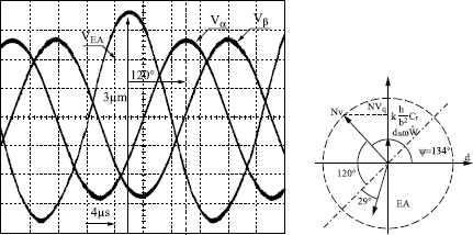
These readings therefore confirm the functioning of the motor, and illustrate the model in the rotating reference frame associated with the traveling wave. As an application example of this model, we propose a torque estimator in the following section.

10.3.5. Torque estimator

The modeling of traveling wave piezoelectric motors shows that the chain of energy conversion linking the torque generated by the motor to the electrical supply is neither simple nor direct. It is, therefore, not conceivable to control an electrical variable to control the torque, like the classical current controls proposed for electromagnetic motors.

However, it is possible to supply a torque estimator, which allows us to know in real time the torque generated by the motor, in order to servo-control or limit it. We describe in this section how to obtain the structure of a torque estimator by inversion of the causal ordering graph in Figure 10.12, which we take again in Figure 10.18 to show only path q as this is the one which carries the torque.

The principle of a torque estimator can be described by the causal ordering graph of Figure 10.19 where we obtain, by inversion of pathways which lead to motor torque C, three different strategies:

– from relationship [10.19], which requires us to know inertia J of the load and its resistant torque Cr;

– by inversion of relationship [10.21] and of the measure of Ω and Ωid which has been proposed by [MAA 97b]; this estimator requires us to know all the torque speed characteristics of the motor;

– from relationship [10.44] and the measure of Vq and .

Solutions 1 and 2 require us to know the speed of the motor. In order to avoid the speed sensor, we will use the solution based on the inversion of relationship [10.44]. However, the inversion of this equation is not direct, because of the differentiated term which has to be evaluated. But if we restrict ourselves to the cases of steady

state or even for functionings in which varies slowly, this term can be disregarded: equation [10.44] then becomes:

[10.48] 

Equation [10.48] then allows us to supply based on the torque estimator:

[10.49] 

This principle has been used on an experimental bench, detailed in Figure 10.20. This bench uses a Shinsei USR30 traveling wave ultrasonic motor 30 mm in diameter, to develop a nominal torque of 0.05 Nm coupled to a DC motor which allows us to impose a resistant torque brake or motor. A torque sensor is also inserted between the load and motor in order to compare the estimation with the torque really developed.

The results of the estimator are shown in Figure 10.21. In this figure, we show the evolution of estimated torque as a function of time when vibration amplitude W is maintained at constant and the load torque Cr is slowly varying in time.

This figure shows that the estimator supplies a reliable value for the motor torque, both in the case of running as a motor (C > 0 when > 0) and as a generator (C < 0 when > 0). This functionality is important because it shows that even if the torque is not a simple function of the electrical supply variables – as is often the case for electrical motors – its estimation is possible without additional sensors to that already present on the motor. It allows us to consider its use in applications with a limited or even controlled torque.

10.4. Control based on a behavioral model

The control of piezoelectric actuators follows two trends: the first, and the most used, consists of considering the behavior of the motor according to the “black box” approach and to compensate for the poorly known and strongly nonlinear effects by online identification methods, and adaptive and/or predictive controllers. The second relies on a physical analysis of the functioning of the actuator and a precise model, although usable in control. This section is linked to the models of the first approach. A summary of the variables for controlling the rotational speed of a traveling wave ultrasonic motor can be found in [NOG 96]. Clearly, the supply frequency, around the resonance, the amplitude of the supply 2-phase voltages and the dephasing between these two voltages are the variables for setting the mechanical variables of the motor. The dephasing between the two supply voltages allows the rotation in one direction or the other, this setting variable therefore is particularly used for the positioning. The relationships between the rotational speed and these variables are however not linear, in particular, the speed-dephasing relationship shows a dead zone around the origin which depends on the load torque [SEN 02]. The speed-frequency relationship also depends on this load torque [PET 00]. Most control strategies rely on one (or even two) of these variables to set the rotational speed of the motor, from the initial online identification of speed-frequency, speed-phase or speed-voltage relationships for given functioning conditions of the motor [CHE 08]. The general approach then consists of approaching the behavior linking the rotational speed (or the position) and the setting variable by a simple function. For instance, in [SEN 02], the authors link the position of the motor to the dephasing of supply voltages by a linear function of second order. Owing to an adaptive control by reference model, they manage to control the position of the rotor; however, the dead zone around the origin not being taken into account for the model control, they call on a fuzzy corrector in order to compensate for it. Fuzzy logic is also used in [BAL 04] to make up for the lack of knowledge on the position-instantaneous frequency model of the motor. A similar approach is developed in [BIG 05], this time using a predictive corrector. Taking into account the nonlinearity brought by this dead zone can finally be done by neuronal identification, as proposed in [CHE 09], or by the exploitation of neuronal and fuzzy methods like in [CHA 03]. Other more thorough research proposes an explicit control of the motor torque [CHU 08]; in this case, the variation range of the torque can even be separated into two parts, one where the motor is supplied with two voltages in phase, the other where the motor is supplied with two voltages in quadrature. In the first part, the motor undergoing a standing wave, it can only offer a resistant torque tuneable according to the supplied voltage, in the second part, it supplies a motor torque. The setting of the torque is ensured by the variation of supplied voltage, according to an initial identification in steady state of the torque characteristics. By performing these methods it may seem that the black box approach knows its limits in terms of practical and industrial implantation, of reproducibility and understanding. They can be helped by a complementary approach which consists of taking advantage of the physical knowledge of the system and relying on knowledge models.

10.5. Controls based on a knowledge model

Less wide spread than the previous ones, these controls generally rely on a coupled analytical model, taking into account the double electromechanical and mechanomechanical conversion which is done in the motor [MAA 00]. The mechanomechanical conversion making tribological phenomena intervene at the stator-rotor contact is often approached for the needs of the control by models which are linearized [GIR 03] or tabulated [MAA 00]. Once these models are put in place, the control consists of inverting the chain of action in order to infer, from the desired references on mechanical variables, the action to be taken on the setting variables.

10.5.1. Inversion principle

This general inversion principle is put into application here via the CIG formalism which illustrates graphically the systematic obtaining of the control structure. The control is based on the inversion principle which consists of defining the input setting according to the desired trajectory of its output in virtue of the principle: find the good cause to generate the good effect. This inversion principle is applied to each elementary sub-system which appears to be a complete model in each chain of action. The control then consists of determining the inverse physical functionality of the process considered [BAR 06]. The inversion method depends on the elementary process to be inverted: if it concerns a rigid processor (time independent), the inversion is direct; for instance:

[10.50] 

If the process is causal (integrally dependent on its input), the direct inversion is replaced with a servo-control of the variable in order to make the real output smes converge to the desired output sref; for instance with a proportional corrector:

[10.51] 

10.5.2. Control structure inferred from the causal model: emphasis on self-control

The causal ordering graph of Figure 10.12 makes two axes to be servo-controlled appear in order to control the motor, normal axis, and tangential axis.

10.5.2.1. Inversion of the tangential axis

Figure 10.22 shows the inversion of path q of the motor in order to control the torque. This control structure is based on the speed control of the ideal rotor Ωid, which is obtained by servo-controlling voltage Vq. Works have allowed us to determine the setting method of the servo-control [DAI 09], which we will not reproduce here.

10.5.2.2. Inversion of the normal axis

We can apply the same method on path d, by inversion of CIG, as on path q. It leads to three strategies, according to the variable controlled:

– Control of the normal speed of the ideal rotor. The inversion of the CIG on path d shows that it is possible to servo-control , the normal speed of the ideal rotor.

However, we have already noticed in equation [10.16] that in the case of an excitation in quadrature of two waves of same amplitude and for the steady state . In fact, another non-zero constant value would make the rotor lift off from the stator, which is a case that is difficult to conceive in practice. We therefore have a limited choice of value of , which has to be at least zero-valued in steady state.

Furthermore, we are not interested in the transient regime on axis d. As a consequence, we will not control this variable, but the controls proposed later will ensure that VNid = 0 in steady state;

– Servo-control of the pulsation of the supplied voltages.

If we carry on the analysis of CIG of Figure 10.12, we notice that is an action variable. Its servo-control is thus possible. Yet, in steady state, = (relationship [10.15]), the pulsation of supplied voltages. It is sometimes interesting to control this pulsation, for instance, for some resonating supplies which show an optimal functioning at a given frequency [MAA 00].

The CIG of Figure 10.24 shows a control structure of this pulsation in axis d.

This graph is made of two interwoven loops. It also requires the compensation of FN, which can be easily done by putting FN = , which is valid in steady

state. Furthermore, an additional simplification of this servo-control is possible, and a calculation method of the correctors used can be found in [GIR 02].

If it is conceivable to servo-control the frequency at a desired value, we have, however, to notice that it cannot be chosen randomly. Too low, it is possible that the motor will stall; too high, the effective value of voltages to apply becomes too large for the supply. Thus, this control must be supplied with an online identification of the resonating frequency, to be able to follow the possible variations due to the temperature. The influence of the resonating pulsation is seen on CIG by intervention of 0. The principle of this control has however been done in practice by [MAA 97b];

– Open loop on path d. We have just mentioned and presented two strategies which implement a setting of Vd by a servo-control loop. In electromagnetic machines, we encounter this configuration where an axis is devoted to the torque control, whereas the other allows us to control another variable, like a flux for instance.

However, this is not always the case: for a synchronous machine with smooth poles, for instance, we set Id = 0, because this allows us to decrease the Joule losses. We can transpose this reasoning in the case of a piezoelectric motor. By noticing that in established steady state, equation [10.44] allows us to write that Vd is constant, we can choose to directly impose Vd = cste. This concerns an open loop control, because no servo-control on path d is undertaken. The choice of this value can be done according to several criteria. For instance, we can choose to work always at resonance, in order to limit the amplitude of the supplied voltages. Then Figure 10.13 shows that in this case, Vd = 0 is the value to impose. Or, some supplies being easy to make if the value of the effective voltages which they deliver remains constant, we can impose constant. The amplitude of voltages vα and will then be equal to V. Let us note, however, that for a given V and Vq, two values of Vd are possible: one is positive and the other is negative. We keep the solution negative, because it makes it possible to work beyond the resonating frequency (Figure 10.13). Let us note that the pulsation of supplied voltages is no longer imposed by the control; it is free not only to evolve according to Vd but also to external conditions. We have simulated in Figure 10.25 the responses in transient regime at a scale interval of Vq, , and frequency of supplied voltages, the effective value of voltages being maintained at constant.

For t = 7.5ms, we impose a variation of −5% of parameter c; this gap simulates a variation of the resonating frequency of the motor under its own over-heating. The fluctuation speed is exaggerated to test the robustness of this strategy with respect to the resonating frequency. We note that this variation is without effect on the value in steady state of . The reason for this is that the frequency of supplied voltages is adapted to the new value of the resonating frequency. We will come back to this property later on.

It is this feature of self-adaptation associated with the simplicity of the supply which led us to choose this control strategy by self-control.

10.5.3. Practical carrying out of self-control

From a practical point of view, the self-control of a traveling wave ultrasonic motor is not an easy thing since the inversion of the rotation matrix must be done at a frequency which is higher than that of the rotating field electromagnetic motors, parameter c of equation [10.15] varying at the frequency of about 40 kHz. However, by noticing that is constant, controlling Vq is done if one controls ψ, the dephasing between the traveling wave and the supplied voltages. That is why, the self-control presented in this chapter is done based on a frequency multiplier with loop and analog phase locking. The principle, represented in Figure 10.26, consists of synchronizing a clock signal SHF with the measure of the voltage coming from the deformation sensor of the motor. This signal, of frequency N times greater than the stator deformation, is the base clock of a counter which counts until N. This counter possesses a load input of adjustable value NΨ, and its output supplies a sinus table which, associated with an external digital analog converter, allows us to generate an alternating sinusoidal voltage which can be written as vα(t). Thus, the frequency of vα(t) is always equal to that of the deformation measure of the motor, whereas the dephasing is a function of

the pre-load input of counter NΨ,. The traveling wave motors being 2-phase, (t) is obtained similarly to (t), but by modifying the pre-load input of the counter of path by adding a quarter of the period (N/4).

The performances of the self-control will be better because the response time of the locking loop will be small, and the number N is large. Better results are obtained with a response time in closed loop of the phase locking loop of 700 µsec, and with N = 128. Thus, the base clock frequency of counters SHF were of the order of 4Mhz; an FPGA solution was then suitable to integrate the set made of two counters, sinus roms and a part of the frequency multiplier.

10.6. Conclusion

The traveling wave ultrasonic motors, without involving electromagnetic fields, ensure a double energy conversion, an electromechanic conversion owing to the indirect piezoelectric effect, then a mechanomechanical conversion through contact. The analytical modeling of these two conversions, by means of certain simplifying hypotheses, emphasizes similarities and a duality with the models classically used for alternating electromagnetic machines. The traveling wave has the role of a rotating field and the position of its maximum can be used to self-control the motor. The use of the representation tool COG allows us to emphasize the decoupled model on two paths d and q, and to analyze the reasons for the stalling of the motor under certain load and supply conditions. As a consequence, the control structure obtained by inversion allows an automatic adaptation of the supply frequency, able to compensate for these phenomena and also to protect us against nonlinear effects because of the thermal drift.

10.7. Bibliography

[BAL 04] BAL G., BEKIROGLU E., DEMIRBAS S., COLAK I., “Fuzzy logic based DSP controlled servo position control for ultrasonic motor”, Energy Conversion and Management, vol. 45, p. 3139-3153, 2004.

[BAR 06] BARRE P., BOUSCAYROL A., DELARUE P., DUMETZ E., GIRAUD F., HAUTIER J., KESTELYN X., LEMAIRE-SEMAIL B., SEMAIL E., “Inversion-based control of electromechanical systems using causal graphical description”, Proceedings of IEEE-IECON, vol. 6, p. 5276-5281, 2006.

[BIG 05] BIGDELI N., HAERI M., “Simplified modeling and generalized predictive position control of an ultrasonic motor”, ISA Transactions, vol. 44, p. 273-282, 2005.

[BUD 03] BUDINGER M., Contribution à la conception et la modélisation d’actionneurs piézoélectriques cylindriques à deux degrés de liberté de type rotation et translation, PhD thesis, INP Toulouse, May 2003.

[CHA 03] CHAU K., CHUNG S., CHAN C., “Neuro-fuzzy speed tracking control of traveling-wave ultrasonic motor drives using direct pulsewidth modulation”, IEEE Transactions on Industry Applications, vol. 39, no. 4, July 2003.

[CHE 08] CHEN T., YU C., TSAI M., “A new driver based on dual-mode frequency and phase control for traveling-wave type ultrasonic motor”, Energy Conversion and Management, vol. 49, p. 2767-2775, 2008.

[CHE 09] CHEN T., YU C., “Motion control with deadzone estimation and compensation using GRNN for TWUSM drive system”, Expert Systems with Applications, vol. 36, p. 10931- 10941, 2009.

[CHU 08] CHUNG S., CHAU K., “A new compliance control approach for traveling-wave ultrasonic motors”, IEEE Transactions on Industrial Electronics, vol. 55, no. 1, January 2008.

[DAI 09] DAI Z., Actionneurs piézo électriques dans des interfaces homme-machine à retour d’ effort, PhD thesis, University of Lille 1, March 2009.

[GHO 00] GHOUTY N.E., Hybrid modeling of a traveling wave piezoelectric motor, PhD thesis, Aalborg University, Department of Control Engineering, May 2000.

[GIR 98] GIRAUD-AudinE C., Contribution à la modélisation analytique d’actionneurs piézo électriques en vue de leur conception et dimensionnement, PhD thesis, INP Toulouse, no. 1501, December 1998.

[GIR 01] GIRAUD F., LEmairE-SEmail B., HautiEr J.-P., “Modèle dynamique d’un moteur piezo électrique à onde progressive”, RIGE, vol. 4, no. 3, p. 411-430, April 2001.

[GIR 02] GIRAUD F., Modélisation Causale et commande d’un actionneur piézeoélectrique à onde progressive, PhD thesis, University of Lille 1, no. 3147, July 2002.

[GIR 03] GIRAUD F., LEmairE-SEmail B., “Causal modeling and identification of a travelling wave ultrasonic motor”, The European Physical Journal Applied Physics, vol. 21, no. 2, p. 151-159, February 2003.

[HAG 95] HAGOOD N.W., McFARLAND A.J. IV, “Modeling of a piezoelectric rotary ultrasonic motor”, IEEE Transactions on Ultrasonics, Ferroelectrics and Frequency Control, vol. 42, no. 2, March 1995.

[HAU 98] HAUTIER J., CARON J., Les convertisseurs statiques: méthodologie causale de modélisation et de commande, Editions Technip, Paris, 1998.

[LU 01] LU F., LEE H., LIM S., “Contact modeling of viscoelastic friction layer of traveling wave ultrasonic motors”, Smart Material Structure, vol. 10, p. 314-320, 2001.

[MAA 95] MAAS J., IDE P., Fröhleke N., GROSTOLLEN H., “Simulation model for ultrasonic motors powered by resonant converters”, IAS ’95, IEEE, vol. 1, p. 111-120, October 1995.

[MAA 97a] MAAS J., GROSTOLLEN H., “Averaged model of inverter-fed ultrasonic motors”, IEEE Power Electronics Specialists Conference (PESC), IEEE, vol. 1, p. 740-786, June 1997.

[MAA 97b] MAAS J., SCHULTE T., GROSTOLLEN H., “Optimized drive control for inverter-fed ultrasonic motors”, IEEE-IAS Annual Meeting, IEEE, vol. 1, p. 690-698, October 1997.

[MAA 00] MAAS J., SCHULTE T., Fröhleke N., “Model-based control for ultrasonic motors”, IEEE/ASME Transactions on Mechatronics, vol. 5, no. 2, June 2000.

[NOG 96] Nogarède B., “Moteurs piézoélectriques”, Techniques de l’ingénieur, vol. D3765, p. 1-20, 1996.

[PET 00] PETIT L., RIZET N., BRIOT R., GONNARD P., “Frequency behaviour and speed control of piezomotors”, Sensors and Actuators, vol. 80, p. 45-52, 2000.

[PIÉ 95] Piécourt E., Caractérisation électromécanique et alimentation électronique des moteurs piézoélectriques, PhD thesis, INP Toulouse, no. 1037, July 1995.

[SAS 93] SASHIDA T., KENJO T., An Introduction to Ultrasonic Motors, Clarendon Press, Oxford, 1993.

[SEN 02] SENJYU T., KASHIWAGI T., UEZATO K., “Position control of ultrasonic motors using MRAC and dead-zone compensation with fuzzy inference”, IEEE Transactions on Power Electronics, vol. 17, no. 2, March 2002.

[TOU 99] TOUHAMI H.O., DEBUS J., BUCHAILLOT L., “Contact modelling by the finite element method: application to the piezoelectric motor”, Journal de Physique IV, vol. 9, p. 217-226, 1999.

[WAL 98] WALLASCHEK J., “Contact mechanics of piezoelectric ultrasonic motors”, Smart Material Structure, vol. 7, p. 369-381, 1998.

---

1 Chapter written by Frédéric GIRAUD and Betty LEMAIRE-SEMAIL.