Chapter 8

Variable Reluctance Machines: Modeling and Control ¹

8.1. Introduction

The term “variable reluctance machine” (VRM) covers a very large range of devices directly or indirectly using the variation of the air-gap permeance to convert electromechanical energy. Different topologies, associated with specific supply modes, have been designed, studied and tested to fulfill the specifications of various applications with very variable performances. Although the majority of structures have not (yet) moved beyond the prototype, two families − synchronous reluctance or synchro-reluctant machines (Synchrel) and the switched reluctance machines (SRM) − have very interesting performances and potentials. The latter already being well established in industry [MUL 99].

The rotors of these two families of machines are devoid of all sources of magnetomotive force (permanent magnets and supplied winding). Only the stator supports polyphase winding (concentrated for SRM and generally distributed for Synchrel). This gives them an undeniable robustness and genuine advantages for high-speed applications. In both cases, synchronous operation can be obtained when their supplies are supervised by an appropriate control. The performances obtained are then comparable, or even greater in some cases, to that of induction machines of the same volume [STA 93].

These machines are not devoid of defects. Thus, the principal drawback of Synchrel machines lies in their power factor, which is relatively limited in the case of basic structures. Its improvement involves the adoption of specific topologies that increase the complexity of manufacture and the price [MEI 86, SAR 81]. On the other hand, SRMs generate a significant pulsating torque inherent to their operating principle. This torque can be decreased by the control but to the detriment of the efficiency of the machine-converter set [HAN 10]. These structures are also known to have vibrations and acoustic noise of magnetic origin. These are due to the action of attractive radial magnetic forces between the stator and rotor teeth, particularly when in conjunction [MIN 08, OJE 09a, OJE 09b]. The advantages of Synchrel and SRM machines, particularly in conjunction position, do however, compensate for their drawbacks, which make them attractive for diverse applications, particularly those at high speeds.

Whichever electromechanical converter is used, a control combining robustness and good performances is dependent, among other things, on an accurate modeling of the machine. The design of the control requires an analytical model of the structure that is developed under a certain number of simplifying hypotheses, which limit its accuracy. A compromise is hence to combine model simplicity and control efficiency. Generally, the saturation of magnetic materials is not insignificant in the case of Synchrel and SRM. This is due to an air-gap, often very weak, feature inherent to these machines. This aspect can possibly be taken into account in the model of the machine.

The current chapter deals with the description, modeling and control of variable reluctance machines belonging to two families: Synchrel and SRMs. It is divided into two parts. Each of them introduces, in the first section, the description and presentation of the operating principle of the structure while introducing the static converter most often used to ensure its supply. The second section of the chapter is devoted to the analytical model of the machine. It uses notions introduced in other chapters about the modeling and control of synchronous machines. The effects more specific to variable reluctance machines (VRM) will be dealt with. Finally, the third section of this chapter will be devoted to different control strategies. In the absence of an excitation circuit, these strategies can significantly differ from those used for classical electromechanical converters. The advantages and limitations of each of them will be emphasized.

8.2. Synchronous reluctance machines

8.2.1. Description and operating principle

The Synchrel machine (SRM) is a structure whose stator, made of laminated steel sheets, is identical to that of a classic synchronous or induction machine with an isthmus of weak opening slots. It is equipped with a polyphase winding with p1 pole pairs that is generally distributed and supplied with a sinusoidal polyphase source to generate a rotating field. The rotor of this machine is salient, with Nr teeth with slots that are usually larger than the stator slots. In its basic version, it can also be made of laminated steel sheets. The transverse cut of an example of a Synchrel machine with Nr= 4 is shown in Figure 8.1.

Due to the disparity in sizes, the effect of the air-gap variation due to the stator slots is ignored and the stator is assumed to be smooth. This hypothesis is widely used in the case of classic machines1 .

The operating principle of the synchronous reluctance machine is based on minimizing the reluctance seen by the armature magnetic field passing by. We can easily show that a synchronous operation, devoid of strong torque ripples, is ensured if Nr and p1 fulfill the following condition [SAR 81]:

[8.1] 

Thus the rotor, having as many teeth as stator poles, will rotate at the same speed as the stator rotating field so that the latter tends to meet a minimum reluctance. From then on, operation is synchronous, with a speed whose expression is given by:

[8.2] 

where represents the supply pulsation of stator variables.

As in the case of a synchronous machine, the Synchrel machine must be supplied according to the position of the rotor. Consequently, a rotor position sensor is necessary. As a matter of fact, this structure is a synchronous machine with salient poles whose excitation circuit has been suppressed [LOU 10]. It therefore only works thanks to the reluctance torque.

As we will see later, the reluctance torque is proportional to the difference between the inductances of direct axis Ld and quadrature Lq under the hypothesis of linearity of the characteristic B(H) of magnetic materials. As a consequence, the increase in the capabilities of this structure (mass torque and power factor) needs to maximize Ld and minimize Lq.

Besides the classical structure in which a minimum air-gap as weak as possible is needed, different other topologies, more or less complex, have been proposed. They sometimes have performances superior to those of squirrel cage induction machines for a same volume. Figure 8.2 shows performances higher to the transverse cut of two of the most interesting topologies in terms of mass torque and power factor − the Synchrel with flux guides [STA 93] and the axially-laminated Synchrel [VAG 00].

Whichever configuration is adopted, the search for optimal Synchrel performance involves a significant level of saturation, which can have a considerable influence on the behavior of these machines.

Synchrel machines are generally supplied by classical pulse width modulation (PWM) inverters. Figure 8.3 shows the converter used in the three-phase case.

Equipped with their converter, the Synchrel machine can, a priori, fulfill the same functions as the squirrel-cage induction machines. Devoid of a rotor coil, they are interesting in terms of manufacturing cost and restricted heating at the rotor. In their classic topology, they suffer from a relatively limited power factor, which is prejudicial to the dimensioning of the static converter. The use of specific rotors (with flux guides or ones that are axially laminated) allows us to considerably improve the power factor, bringing it closer to that of classic induction machines, but this is done at the expense of manufacturing price. As a rule of thumb, these structures are limited to low- or medium-power applications.

Due to the absence of a rotor circuit, these machines are well adapted to highspeed operations. In this case, they are often equipped with a massive rotor where currents are induced during the transient operations. This phenomenon needs to be taken into account in the modeling of the machine.

Whichever application is targeted, it is necessary to control the structure through the control of the static supply converter. The design of the control of the system machine-converter needs a model of the set. The following section is devoted to the mathematical model of the Synchrel machine.

8.2.2. Hypotheses and model of a Synchrel machine

As previously mentioned, the Synchrel machine can be considered as a synchronous machine with salient poles without an excitation circuit. As a consequence, its model can be directly inferred from that of this structure. For the sake of simplification, we only show the classic model of this machine. We will be able to refer to other works to take into account the saturation phenomenon and/or currents induced in a massive rotor [LUB 03, TOU 93].

By adopting the simplifying hypotheses (see section 1.3.2 and the notations in 1.3.3 of [LOU 10]) devoted to modeling in view of the control of synchronous actuators, the matricial equation ruling the electrical variables of the stator of a three-phase Synchrel machine is written in the following form:

[8.3] 

where Rs is the phase resistance and (3), (i3) and (3) represent the voltage, current and flux vectors, respectively, relative to the stator phases of the machine.

The flux vector can be written in the following form:

[8.4] 

where (Lss()), the inductance matrix, is expressed as:

[8.5] 

with being the mechanical position. The classical development of Lss0 and (Lss2()) [LES 81] is given in Chapter 1 of [LOU 11].

The expression of electromagnetic torque developed by the structure is obtained directly from the derivative of the coenergy, which leads to:

[8.6] 

Since there is no excitation circuit, the stator currents are used for magnetization of the machine and generation of torque at the same time. This differs from the case of the synchronous machine in which the excitation current (or magnets in the case of a PMSM) plays a dominant role. However it is possible to supply the machine with a strategy similar to that of self-controlled synchronous machine.

The study and control of Synchrel machines are usually done using the diphase model. To develop this model, we use the Park transform of angle p1 (see Chapter 1 of [LOU 11]). We then obtain the expressions of the different electrical variables, given in the referential linked to the rotor. Thus, by applying this transform to equation [8.3], the latter is re-written in the following form:

[8.7] 

where d, q, id and iq, respectively, represent the stator voltages and currents according to direct d and in quadrature q axes. d and q, the fluxes according to these same axes, are expressed:

and:

where Ld and Lq are the direct inductance and the inductance in quadrature, that are written in a manner similar to those of the synchronous machine with salient poles, i.e.:

and:

The same transform, applied to relationship [8.6], leads to the following expression of the electromagnetic torque:

[8.8] 

8.2.3. Control of the Synchrel machine

Control of the Synchrel machine is based on the vector control approach through the variables expressed in referential d − q. The electromagnetic torque is proportional to the product of stator currents id and iq, as shown by relationship [8.8]. We then have a degree of freedom in the choice of currents since, only the product is imposed for a given load torque. Several control strategies exist [BET 93]. They are distinguished by the criterion to be optimized during the generation of current references. In fact, we can control the Synchrel machine in order to maximize a criterion, such as the efficiency output [LUB 03], power factor [BOL 96] or electromagnetic torque [BET 93]. The global diagram of speed control is given in Figure 8.4.

From the speed reference and a corrector , we can determine the reference torque of the machine. According to the control strategy adopted, we infer the reference values of currents id and iq. The regulation loops of currents id and iq (correctors Cd(s) and Cq(s)) and the inverse Park transform allows us to end up with the three-phase reference voltages that the PWM inverter must generate.

In the following, we will present the most common control strategies. To illustrate them, we will show the simulation results for a machine with cut sections, represented in Figure 8.1, whose electrical and mechanical parameters are given in Table 8.1. J represents the inertia moment of the system and f the viscous friction coefficient. The inductances Ld and Lq can be measured using the voltage scale interval method (current response) by positioning the rotor according to axis d or q.

8.2.3.1. Vector control with id constant

In the applications that need good dynamics at low speed (quick torque response), we often prefer to control the Synchrel machine using a constant current id [BET 93]. This allows us to impose flux in the machine, since the inductance of axis d (small air-gap) is large compared to that of axis q (large air-gap). The principle of this control is similar to that of a DC machine with separate excitation. The component the of stator current along axis d, playing the role of excitation, allows us to set the value of the flux in the machine (nominal flux dn). The component along axis q plays the role of the armature current and allows us to control the torque. The torque can then be written:

[8.9] 

with:

[8.10] 

and:

[8.11] 

This strategy allows performant drive systems to perform and enables us to impose the nominal torque, from stand-still to nominal speed.

The control strategy block shown in Figure 8.4 can be completed by that of Figure 8.5. Current idref has a constant value corresponding to the rated flux in the machine (equation [8.11]). The reference value of the current iqref is determined according to the type of control used in the application (speed or torque). In the case of speed regulation, iqref is obtained through a speed corrector. It is limited to ensure the protection of the machine in terms of current magnitude.

The block diagram of the stator current’s regulation loop along axis d is given in Figure 8.6 (the regulation loop according to axis q is identical to within the indices). To synthesize the correctors (generally of porportional integral (PI) controller type), we re-write equations [8.7] in the following form:

[8.12] 

[8.13] 

These relationships make the coupling terms p1Lqiq and p1Ldid appear between the two axes. They are considered perturbations that need to be compensated for by the control (estimated term, ẽq). The corrector gains are calculated using the classic automatic methods.

Figure 8.7 shows the block diagram of speed regulation. The transfer function of the system is obtained from the fundamental relationship of the dynamics of rotating systems:

[8.14] 

where Cch represents the load torque. Coefficient K (torque coefficient), which appears in Figure 8.7, is defined by equation [8.10].

The structure of the speed corrector is of PI controller type. To calculate the value of the speed corrector gains (Kp and Ki), we assume that current iq instantaneously follows its reference (this hypothesis is often fulfilled due to the difference in the time constants of the speed loop and the current loop).

The results of applying this control strategy to the case of simulation will be presented in section 8.2.3.4.

8.2.3.2. Maximum torque control

Stator current vector is can be represented in referential d − q linked to the rotor (Figure 8.8). In steady state, it is fixed and has a constant norm in this referential.

We can then define angle, , referred to as the control angle, as well as variable m, so that:

[8.15] 

The control strategy consists of determining the value of m (or ) in order to obtain the maximum torque for a given stator current value.

The expression of electromagnetic torque is:

[8.16] 

The root mean square (RMS) value of the current in one phase of the stator can be expressed as:

[8.17] 

By using this relationship in expression [8.16], we can express the electromagnetic torque as a function of is and coefficient m:

[8.18] 

We can then show that the machine develops the maximum torque for a given current if the following condition is fulfilled:

[8.19] 

In this case, the expression of the maximum torque is:

[8.20] 

The optimum control angle therefore has as a value of /4, which corresponds to id = iq. It is then sufficient to use this equality in the control for the machine to operate at its maximum torque. The current absorbed is then at a minimum for a given torque, which minimizes Joule losses in the machine.

In the case of this strategy, the control block of the diagram in Figure 8.4 can be completed by that of Figure 8.9.

8.2.3.3. Maximum power factor control

By disregarding the different losses in the machine, the power factor can be defined as the ratio of the converted mechanical power to the apparent power:

[8.21] 

where Vs, the RMS voltage of a stator phase, can be written in the following form by disregarding the voltage drops:

[8.22] 

By expressing flux s as a function of its components according to axes d and q:

[8.23] 

we end up with the following expression of the power factor:

[8.24] 

With regard to m, the power factor is at its maximum for:

[8.25] 

This only depends on the ratio of Ld/Lq, as can be seen below:

[8.26] 

The control strategy block of the diagram of Figure 8.4 can then be completed by that of Figure 8.10:

8.2.3.4. Simulation results

In Figure 8.11, we present the simulation results obtained for the control strategy with id constant. The calculations have been done by using the electrical and mechanical parameters given in Table 8.1. The value of current idref is set at 2.5 A. At t = 0.5 s, a speed level of 400 rpm is applied. It induces a current draw iq of 7.0 A (we notice that current iq enters into the limitation). An anti-windup device is put in place to avoid non-negligible draw when current iq is limited. At t = 2.0 s, a load torque level of 4 N.m is applied. The rotational speed drops slightly and stabilizes again around 400 rpm. We notice that current id is barely disrupted by the variations in iq.

Figure 8.12 shows a comparison between the different control strategies in terms of Joule losses and power factor by considering the complete model of the machine. The operating point is the same as that in Figure 8.11 (400 rpm, 4 N.m). At t = 4.0 s, we go from the control strategy at constant id to the control strategy at maximum torque. At t = 5.0s, we use the control strategy at maximum power factor. We notice that the Joule losses are at a minimum for the second control strategy and that the maximum power factor obtained is Fp = 0.44. For the machine studied here, with the saliency ratio Ld/Lq being weak (Ld/Lq = 2.6), the maximum power factor is relatively limited.

Finally, Figure 8.13 represents the variations of the power factor as a function of saliency ratio Ld/Lq (this ratio depends on the structure of the machine) for a control strategy at maximum power factor and a control strategy at maximum torque (m = 1). In the case of the control strategy at maximum power factor, we observe that the latter becomes interesting for supply dimensioning (static converter) from a saliency ratio > 6.

8.2.4. Applications

The controlled Synchrel machine has a very interesting performance. Except for the limited power factor in classic structures that can largely be improved by adopting specific rotors, the machine’s performance can be comparable to that of induction machines. References mentioning its use in industrial applications are rare, although it is present in some catalogs produced by manufacturers of electrical machines for powers up to a few kW [ISG 11, LUC 04, SAV 99].

8.3. Switched reluctance machines

8.3.1. Description and principle of operation

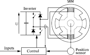
The switched reluctance machine (SRM) consists of a stator and a rotor with laminated steel sheets equipped, respectively, with Ns and Nr teeth that are regularly distributed. The magnetic circuit of the rotor is totally passive (there are no conductors or magnets); whereas the stator supports the armature winding. Thus, a concentrated coil is wound around each tooth. The coils surrounding diametrically opposed teeth, in the electrical sense, are connected to create a winding of q phases with p1 pole pairs. Figure 8.14 shows an example of a SRM structure. It possesses eight stator teeth and six rotor teeth. The armature winding, with four phases, has one pole pair.

SRM operation can easily be made explicit. Similarly to the current in an electrical circuit trying to follow the path with the lowest impedance, the flux in a SRM tries to follow the easiest path between two points. As a consequence, when the winding of one phase is supplied, the electromagnetic field generated is going to attract the closest rotor tooth, so that it tends to align along the axis of the phase in order to minimize the flux path in the air and apply the maximum flux rule in the magnetic circuit: this is the reluctant effect. To ensure “continuous” running, it is enough to sequentially supply the phases (one phase after the other) to attract the closest rotor tooth as it goes along. It is easy to understand the need for a position sensor to ensure the supply. SRM operation does not require a rotating field, so the coils are ideally supplied with current pulses. The current pulses can be unipolar or bipolar square-wave current. In fact, reluctance minimization is independent of the field polarities.

In both cases, in order for the operation described above to be possible, the following relationship, between Ns, Nr and p1, has to be fulfilled:

[8.27] 

When a unipolar (or bipolar) supply of phases occurs periodically, at pulsation , the rotor moves at a speed :

[8.28] 

During rotation of the rotor, two particular positions are distinguished, which are very important in the modeling and control of the SRM (see Figure 8.15):

– The opposition position: for which the stator and rotor teeth are furthest away from each other. As a consequence, the magnetic circuit has a minimum inductance (maximum air-gap).

– The conjunction position: for which the stator and rotor teeth are facing each other. The magnetic circuit shows a maximum inductance.

These two positions confine the energy cycle for a given current magnitude, as shown in Figure 8.16.

It is possible to show that the average electromagnetic torque <Cem,k> generated by a phase is proportional to the surface W of this cycle as well as the number of rotor teeth Nr [KRI 01, MIL 01]:

[8.29] 

As a consequence, for a given number of teeth and level of current, the torque is a function of the difference between the flux in conjunction position and in opposition position. The difference between these two fluxes must be as high as possible which implies the weakest minimum air-gap possible.

As mentioned previously, the SRM is generally supplied with unipolar square-wave current. The most frequently used converter then consists of an asymmetrical half-bridge per phase (see Figure 8.17).

The arms being controlled independently of each other, in the case of a defect on a component, the functioning of the other bridges is not interrupted [GAM 08]. In this case, the control angles must be recalculated in order to maximally decrease the torque ripples and optimize the global efficiency of the set machine/converter.

The SRM has for a long time been used in applications requiring step-by-step operation. Due to its low cost and high robustness, as well as the advances in power and control electronics, it is increasingly being used in applications similar to those of classic structures; it is particularly appreciated in industrial applications requiring high-speed running (alterno-starter, high-speed machining, etc.) [VIS 04, VRI 01]. However, its composition and principle of operation require very specific modeling and control with respect to other synchronous machines.

8.3.2. Hypotheses and direct model of the SRM

The SRM is a structure whose phase windings are, in the majority of cases, magnetically independent. We can therefore write the following electrical equation for each of the phases of the machine:

[8.30] 

where Rs is the phase resistance. u, i and represent the voltage at the terminals, the current and the total linkage flux of the phase winding, respectively. The latter is function of current i and the position of the rotor , as shown in the Figure 8.18, drawn for a 8/6 SRM.

By adopting the hypothesis of a linear magnetic material behavior, it is possible, at first, to express the linkage flux as a function of inductance in the form:

[8.31] 

Electrical equation [8.30] then becomes:

[8.32] 

In the case of unsaturated operation of the magnetic circuit, phase inductance L(,i) varies only according to position. The coenergy [LOU 04, MAT 04] is then written as:

[8.33] 

We then infer the expression of the electromagnetic torque generated by a phase supplied with a constant current i:

[8.34] 

The equation of torque allows us to make a few fundamental observations:

– as the sign of the torque is independent of the direction of the current, unipolar square-wave currents are often used;

– the machine can run as a motor (dL/d) > 0 or as a generator (dL/d) < 0.

The torque generated by the different phases is equal to the algebraic sum of torques generated by each of the q phases:

[8.35] 

In practice, the non-saturation hypothesis of the magnetic circuit is invalid; the phase inductance is a function of the position of the rotor and the phase current. In this case, the electrical expression becomes:

[8.36] 

The expression of the electromagnetic torque is obtained by a derivative of the coenergy with respect to the position, namely:

[8.37] 

The evolution of the inductance and/or torque can be expressed by an analytical expression or via a two-dimension table. Then, these analytical expressions or tables can be integrated in the machine’s control laws (see section 8.3.3.1).

Figure 8.19 represents the behavior of the torque generated by a phase as a function of the position and magnitude of the supply current of a SRM. The nonlinear feature of these characteristics gives us an insight into the difficulties of controlling this structure.

8.3.3. Control

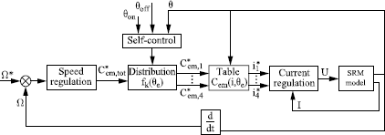
Contrary to other machines, the SRM only operates when it is self-controlled. The global structure of the control is generally made of q fast internal current regulation loops and one external speed regulation loop, as shown in Figure 8.20.

The (linear or nonlinear) speed corrector has as output the total torque reference. The latter can be distributed over the q phases in two different ways, which will be detailed in the following sections. The conversion of the torque reference C*tot into a reference current is the most important and specific part of control in the SRM.

As a rule of thumb, the phases of the SRM are supplied, according to the rotor position, in order to generate the required torque: it is self-controlled. We then distinguish two setting parameters (see Figure 8.21) established with respect to the inductance variation of one phase:

– start angle on: this is the electrical angle at the beginning of magnetization with respect to the opposition position. It corresponds to the switch-on time of the switches;

– the electrical angle at the end of magnetization, written as off.

The period during which the phase is supplied is the “magnetization period”. It is written as p and is equal to off − on.

Figure 8.22 shows an example of the supply sequence of the windings of a SRM with four phases (q = 4) during an electrical period. The impulses are shifted by 2π/q radians. In this example, the start angle on is π/6 and the end of magnetization angle off is 5π/6, namely p equal to 2π/3.

The torque being indirectly controlled through current regulation, the transformation of the total reference torque, obtained from the output of the speed regulator, into q reference currents can be done in two ways:

– one, referred to as “instantaneous torque control” (ITC), aims for the generated torque to follow instantaneously the reference torque. In this case, the reference current of the conduction phase is calculated at each sampling period in order to ensure this equality;

– the other is referred to as “average torque control”. In this case, the average value of the generated torque must be equal to the reference torque. This leads to reference currents in the form of pulses.

The choice of control type depends on the goals of the application being considered. These aims can be: the minimization of torque ripples; the maximization of efficiency; the maximization of torque at high speed; etc.

8.3.3.1. Instantaneous torque control

In this approach, total reference torque is at first distributed on the phases in conduction according to the self-control (on, off and ) and according to a distribution law. From the one-phase reference torques thus obtained and measure of the position, the reference currents are calculated by using a torque table Cem (, i) (see section 8.3.2 and Figure 8.19 (bottom)) generally obtained by finite element calculations or experimental tests. Linear interpolations allow us to infer the reference current of each phase as a function of the electrical position of the rotor and the reference torque per phase.

By assuming current regulators with a sufficiently large bandwidth, this method has the advantage of considerably minimizing the torque ripples because the torque is instantaneously controlled. The goal thus amounts to finding the best reference current profile (i.e. to how best to distribute the total reference torque over the q phases) that allows us to reach the required torque and to optimize one or more goals, such as Joule losses and/or torque ripples [KJA 97].

A first solution consists of sequentially imposing the reference torque on each of the phases. Calculation of the reference current of the active phase can then be obtained in two different ways:

– In the hypothesis of a phase inductance, which can be modeled using a trigonometric function L(,i) ≈ L0 + L1cos() with L0 and L1 two positive constants, the expression of the electromagnetic torque can be written as (see section 8.34). In order to ensure the equality between generated torque Cem,k and reference torque , the reference current is calculated as follows:

[8.38] 

— Generally, the phase inductance cannot be modeled by such a trivial trigonometric function, given the strong saturation feature of the machine. In this case, the reference current is obtained from a two-dimensional torque table, as shown in Figure 8.23 below, and the use of linear interpolations.

However, these solutions are not advocated because of strong torque ripples as well as the increase in Joule losses.

An alternative consists of sharing the total requested torque between two successive phases over a large range in order to decrease the quite significant torque ripples at commutation times [KRI 01]. Generally, the torque is distributed over the q phases in the following way:

[8.39] 

where fk and are the distribution function and the torque reference of the kth phase, respectively. Several functions can play the role of fk (e) [KRI 01, MIL 01]. A possible solution, represented in Figure 8.24, consists of manipulating the trigonometric functions so that:

[8.40] 

with:

The choice of angles on and off of the self-control directly affecting the profile of the reference current, the commutation from one phase to the other must be done over a sufficiently long duration Δ in order to ensure a progressive transfer of the total torque. Furthermore, in motor operation with the adopted logic of torque distribution, it is necessary that the conduction takes place during the phase inductance growing (generation of a positive torque). We then have an additional condition:

[8.41] 

The global block diagram of control, in the case of the instantaneous torque control, is given in Figure 8.25.

The regulation of currents is generally ensured by a hysteresis regulator for simplicity of design, although it introduces strong current ripples and hence torque ripples in steady state. An alternative consists of adding a linear or nonlinear regulator associated with a PWM.

8.3.3.2. Average torque control

The ATC is the method most often used to control torque. The phases are supplied by current pulses of constant value that generate a strongly rippled instantaneous torque whose average value is equal to the reference torque.

The three setting variables are: on, off and the reference current Iref. Several combinations of these variables can generate the same average torque at a given speed. The choice of their values can be done through the optimization of various objectives, such as the efficiency or ripple rate according to the type of application desired. The setting variables are then stored in two-dimensional tables [HAN 08, HAN 10, REK 07].

Once reference current Iref, as well as angles on and off are determined, the regulation of currents is ensured in the same way as for ITC.

The global block diagram of ATC is shown in Figure 8.27.

8.3.3.3. Comparison of the two controls

In order to illustrate the assertions of the last two sections, Figure 8.28 shows the comparison of the two types of control in steady state with a 5.4 N.m. load. In the case of ATC, the reference current is constant; whereas it is modulated in the case of ITC, which allows us to decrease the torque ripples.

The performances of the ITCs depend on the exact measure of the position and dynamics of current regulation chosen. The current in the phase must be able to perfectly follow its reference; otherwise it generates significant torque ripples, mainly at the commutation time.

These limitations are essentially due to the supply source. In fact, when the speed increases, the electromotive force (emf) increases, which decreases the di/dt ratio for a given supply voltage. In the end, the current can no longer reach Iref and the voltage applied to the phase is saturated at its maximum value, which corresponds to the operating mode referred to as “full wave”. Torque control is then only achieved by variation in angles on and off; the ITC then becomes the ATC.

The condition imposed by equation [8.41] is another source of limitation for the ITC. An anticipated commutation where angle on is negative is not possible in instantaneous control. The advantage of such a commutation lies in the fact that it allows the current to increase quickly while the inductance is weak. When the current is already well-established in the phase, it generates a high torque that compensates for the negative torque generated at the beginning of the magnetization phase.

From the point of view of practical implantation, the memory space occupied in the case of ATC is larger because it involves manipulating three tables of optimal parameters versus one table in the case of the ITC. On the other hand, the number of arithmetic operations is larger for the ITC, where there are one or (at most) two functions to perform, besides the linear interpolations. The principal elements of this comparison are summarized in Table 8.2.

Table 8.2. Comparison algorithmic cost – the memory site for the two methods

	Instantaneous torque control	Average torque control
Memory space	1 table C(,i)	3 tables on, off, Iref
Algorithmic cost	2 function cosine at most (generally 2 phases are supplied simultaneously) + 4 interpolations (1 per phase)	3 linear interpolations
Torque ripple	Small	Large
Dependence of the position	Calculation of current references at each sampling period according to the torque and position reference	Reading of the current reference at each sampling period according to the torque reference and the speed
Torque/speed plane	Decreased surface	Increased surface
Peak phase current	Greater than with the ATC, for an equal RMS current	-

The ITC is then better for applications that do not tolerate torque ripples (machine tools [VIS 04] or robotics) with high performance restricted to a certain range of running. As opposed to the ITC, the ATC is able to cover the whole torque/speed plane of the machine, but with limited performance. The ATC is essential in order to exploit the performance of the machine (maximize the torque, efficiency, etc.).

8.3.3.4. Continuous conduction

Figure 8.29 shows the energy cycle in plane (,i) for two different speeds: 500 and 5,000 rpm. The quantity of potentially useable energy is delimited by two flux curves at the opposition and conjunction positions. The energy conversion is better at 500 rpm, where almost all the surface is used. This is not the case at 5,000 rpm where the energy cycle is greatly reduced with respect to the quantity of potentially useable energy. In fact, at high speed and with a constant voltage source, the emf induces an unavoidable current drop in the phase.

The decrease in energy converted per phase causes a torque and power drop from the nominal speed of the SRM according to equation [8.29]. In order to increase the torque at high speeds, we can decrease the number of coils per phase. However, this solution leads to a decrease in torque at low speeds [HEN 06, REK 07, REK 08, SCH 09]. A second solution consists of supplying the SRM without demagnetizing the phases at each cycle: it is what is referred to as “continuous conduction” (see Figure 8.30). Work carried out on this operating mode has been very recent, although the advantages of an “excitation” (a continuous component) have been known for a long time [MUL 94].

Continuous conduction is done by increasing conduction angle p at values greater than 180°: the fact that angle p is greater than half an electrical period (180°) can lead to an incomplete demagnetization of phases and hence a progressive growing of the flux and current. The risk in this operating mode is that we can lose control of the current which carries on increasing until the protection system is set off. High-performance control of the current is necessary to control the divergence risks [HAN 08, IND 05, LOU 06, REK 07]. A possible solution consists of adjusting the magnetization duration p through an efficient control of the current. See Figure 8.31 [HAN 08].

However, this type of supply has drawbacks, namely [HIL 09]:

– a decrease in the global efficiency of the set machine/converter, essentially due to Joule losses;

– an increase in torque ripples due to sensitivity of the control to an update of the mechanical position (self-control of the machine). As a consequence, a relatively short sampling period is necessary (in the range of 1 to 20 µs).

To conclude, continuous conduction is an excellent way to increase the power peaks without increasing the nominal power of the machine.

8.3.4. Applications

Here we consider applications using industrial drives at variable speeds, from large-scale economy drives (household appliances) to high-performance drives (aeronautics, the motor industry, etc.).

In the naval propulsion field, compactness and greater maneuverability are the improvements looked for. Thus, the SRM has been used to create naval propulsion units of 7.5 kW or 2.2 kW [MAR 00, RIC 96a].

The SRM fulfills the demands of the aeronautical world [NAA 05, RAD 92]. In planes, or even helicopters, work has been carried out to design alterno-starters that are directly coupled to the turbine. General Electric [RIC 96b] has worked on a device represented in Figure 8.32 whose features are the following: 177 N.m from 0 to 13,500 rpm and 250 kW at steady state from 13,500 to 22,200 rpm (330 kW peaks during 5.0 s). It has been chosen for its operating qualities in extreme environments (high temperatures) and for its tolerance to defects (it can run in degraded modes).

The SRM, being robust by design, has therefore naturally attracted the attention of motor industry manufacturers, both for use as a motor and as a generator. The studies and publications on this topic are numerous [FAH 04, FAI 05, KAL 02, KRI 06, RAH 00, RAH 02, WU 02, ZHU 07]. The typical application is the alterno-starter [FAH 04, FAI 05]. It is coupled to the thermal motor and can also be used as a traction motor in hybrid vehicles, thus allowing the recovery of braking energy.

Prototypes of hybrid vehicles having the SRM as a traction motor have been built in Australia. The Commonwealth Scientific and Industrial Research Organisation has worked with the Australian motor industry to develop two hybrid prototypes, one with parallel structure (ECOmmodore [HOL]) and the other with a structure in series (aXcessaustralia LEV [AXE]). SR Drives in partnership with Green Propulsion, a Belgian company specialized in the development of clean vehicles, has designed two SRMs (50 kW and 160 kW, see Figure 8.33) for a project involving hybrid propulsion of a bus [SRD].

The SRM has also been used in certain domestic applications, due to its cost and ergonomy [MUL 99]. We can cite, for example, the motors of Neptune of Maytag washing machines or those marketed by SR Drives.

The SRM is also used in many other types of applications or products, such as pumps, compressors, sliding doors, in robotics, etc. [SRD].

To finish, let us cite a few manufacturers who market this machine, such as Allenwest, Brighton Ltd in the UK, Sicme-Motori in Italy [MUL 94] and SRD Ltd in the UK, which is a subsidiary of Emerson Electric Company in St. Louis, Missouri.

8.4. Conclusion

This chapter has been devoted to the description, modeling and control of the two most common families of variable reluctance machines, namely Synchrel machines and SRMs. In both cases, the structures have been tackled similarly by starting with a brief description of the generic topology and a description of the principle and operating conditions. The analytical models that have been developed, often under not insignificant simplifying hypotheses, are those that are most often used to study operation and establish control laws. The control procedures presented are those that are the most common or the most frequently studied. Finally, where possible, care has been given to the introduction of examples of machines used in industry.

This chapter in no way aims to provide an in-depth study of these two families of machines, but rather a “simplified” presentation of these structures and their associated controls in order to give an idea of their controlled operation.

In fact, these machines are still a topic of research today, from a topological point of view and with regards to their supply and control. The content of this chapter, as a consequence, is far from being exhaustive, and different aspects (saturation effects, induced currents, vibrations, noises, etc) have been omitted.

8.5. Bibliography

[AXE] http://www.csiro.au/solutions/aXessaustralia.html

[BET 93] BETZ R.E., LAGERQUIST R., JOVANOVIC M., MILLER T.J.E., MIDDLETON R.H. “Control of synchronous reluctance machine”, IEEE Transactions on Industry Applications, vol. 29, no. 6, pp. 1110-1122, 1993.

[BOL 96] BOLDEA I., Reluctance Synchronous Machines and Drives, Clarendon Press, Oxford, 1996.

[FAH 04] FAHIMI B., EMADI A., SEPE R.B. Jr., “A switched reluctance machine-based starter/alternator for more electric cars”, IEEE Transactions on Energy Conversion, vol. 19, no. 1, pp. 116-124, 2004.

[FAI 05] FAIZ J., MOAYED-ZADEH K., “Design of switched reluctance machine for starter/generator of hybrid electric vehicle”, Electric Power Systems Research, vol. 75, no. 2-3, pp. 153-160, 2005.

[GAM 08] GAMEIRO N.S., CARDOSO A.J.M., “Fault tolerant control strategy of SRM drives”, International Symposium on Power Electronics, Electrical Drives, Automation and Motion, SPEEDAM’08, pp. 301-306, June 2008.

[HAM 09] HAMITI M. O., Réduction des ondulations de couple d’une machine synchrone à réluctance variable. Approches par la structure et la commande, PhD thesis, Nancy I University, France, June 2009.

[HAN 08] HANNOUN H., Etude et mise en œuvre de lois de commande de la machine à réluctance variable à double saillance, PhD thesis, Paris-sud XI University, Gif-sur-Yvette, France, October 22, 2008.

[HAN 10] HANNOUN H., HILAIRET M., MARCHAND C., “Design of a SRM speed control strategy for a wide range of operating speeds”, IEEE Transactions on Industrial Electronics, vol. 57, no. 9, pp. 2911-2921, 2010.

[HEN 06] HENNEN M.D., BAUER S.E., DE DONKER R.W., “Influence of continuous conduction mode on converters in SRM drives”, 22nd International Electric Vehicle Symposium, (EVS22), pp. 1848-1857, Yokahoma, Japan, October 2006.

[HIL 09] HILAIRET M., HANNOUN H., MARCHAND C., “Design of an optimized SRM control architecture based on a hardware/software partitioning”, 35st Annual Conference of IEEE Industrial Electronics Society (IECON'09), November 2009.

[HOL] http://www.holden.com.au.

[IND 02] INDERKA R.B., MENNE M., DE DONCKER R.W.A.A., “Control of switched reluctance drives for electric vehicle applications”, IEEE Transactions on Industrial Electronics, vol. 49, no. 1, pp. 48-53, 2002.

[IND 05] INDERKA R.B., KEPPELER S., “Extended power by boosting with switched reluctance propulsion”, 21th International Electric Vehicle Symposium, (EVS21), Monaco, April 2005.

[ISG 11] http://www.isgev.com.

[KAL 02] KALAN B.A., LOVATT H.C., PROUT G., “Voltage control of switched reluctance machines for hybrid electric vehicles”, IEEE Power Electronics Specialists Conference PESC’02, vol. 4, pp. 1656-1660, June 2002.

[KES 02] KESTELYN X., FRANÇOIS B., HAUTIER J.P., “Torque estimator for a switched reluctance motor using an orthogonal neural network”, Electrical Engineering Research Report, no. 14, pp. 8-14, 2002.

[KJA 97] KJAER P.C., GRIBBLE J.J., MILLER T.J.E., “High-grade control of switched reluctance machines”, IEEE Transactions on Industry Applications, vol. 33, no. 6, pp. 1585-1593, 1997.

[KRI 06] KRISHNAMURTHY M., EDRINGTON C.S., EMADI A., ASADI P., EHSANI M., FAHIMI B., “Making the case for applications of switched reluctance motor technology in automotive products”, IEEE Transactions on Power Electronics, vol. 21, no. 3, pp. 659-675, 2006.

[KRI 01] KRISHNAN R., Switched Reluctance Motor Drives: Modeling, Simulation, Analysis, Design and Applications, CRC Press, 2001.

[LES 81] LESENNE J., NOTELET F., SEGUIER G., Introduction à l’Électrotechnique Approfondie, Technique et Documentation, Paris, France, 1981.

[LOU 06] LOUDOT S., “Method for controlling a heat engine vehicle driving assembly”, International Patent, W0 2006/05028 A2, 2006.

[LOU 04] LOUIS J.-P., FELD G., MOREAU S., “Modélisation physique des machines à courant alternatif’”, in: LOUIS J.-P. (ed.), Modélisation des Machines Électriques en vue de Leur Commande – Concepts Généraux, Traité EGEM (Série Génie Electrique), HermesLavoisier, Paris, France, 2004.

[LOU 11] LOUIS J.-P., FLIELLER D., NGUYEN N. K., STURTZER G., “Synchronous Motor Controls, Problems and Modelling”, in LOUIS J.-P. (ed), Control of Synchronous Motors, ISTE-Wiley, 2011

[LUB 03] LUBIN T., Modélisation et commande de la machine synchrone à réluctance variable, prise en compte de la saturation, PhD thesis, Nancy I University, France, April 18, 2003.

[LUC 04] LUCAS-NÜLLE SOCIETY, Catalogue of the LUCAS-NÜLLE Society, EEM Machines Électriques, 2004.

[MAR 00] MARGOT J.P., YECHOUROUN C., MARMET R., GALSTER P., “Entraînement avec moteur à réluctance variable”, Electronique de Puissance du Futur, Lille, France, November 29−December 1, 2000.

[MAT 04] MATAGNE E., DA SILVA GARRIDO M., “Conversion d’énergie : du phénomène physique à la modélisation dynamique”, in: LOUIS J.-P. (ed.), Modélisation des Machines Électriques en vue de Leur Commande – Concepts Généraux, Traité EGEM (Série Génie Electrique), Hermès-Lavoisier, Paris, France, 2004.

[MEI 86] MEIBODY-TABAR F., Etude d’une machine à réluctance variable pour des applications à grande vitesse, PhD thesis, INPL, Nancy, France, 1986.

[MIL 01] MILLER T.J.E., Electronic Control of Switched Reluctance Machines, Newnes Power Engineering Series, 2001.

[MIN 08] MININGER X., LEFEUVRE E., GABSI M., RICHARD C., GUYOMAR D., “Semiactive and active piezoelectric vibration controls for switched reluctance machine”, IEEE Transactions on Energy Conversion, vol. 23, no. 1, pp. 78-85, 2008.

[MUL 94] MULTON B., Conception et alimentation électronique des machines à réluctance variable à double saillance, thesis, Ecole Normale Supérieure de Cachan, 1994.

[MUL 99] MULTON B., BONAL J., “Les entraînements électromécaniques directs: diversité, contraintes et solutions: la conversion électromécanique directe”, Revue de l'Électricité et de l'Électronique, no. 10, pp. 30-31 and pp. 67-80, 1999.

[NAA 05] NAAYAGI R.T., KAMARAJ V., “Shape optimization of switched reluctance machine for aerospace applications”, 31st Annual Conference of IEEE Industrial Electronics Society IECON’05, pp. 168-173, November 2005.

[OJE 09a] OJEDA X., HANNOUN H., MININGER X., HILAIRET M, GABSI M., MARCHAND C., LÉCRIVAIN M., “Switched reluctance machine vibration reduction using a vectorial piezoelectric actuator control”, EPJ Applied Physics Journal, vol. 47, pp. 31103, 2009.

[OJE 09b] OJEDA X., MININGER X., BEN AHMED H., GABSI M., LECRIVAIN, M., “Piezoelectric actuator design and placement for switched reluctance motors active damping”, IEEE Transactions on Energy Conversion, vol. 24, no. 2, pp. 305-313, 2009.

[RAD 92] RADUN A.V., “High-power density switched reluctance motor drive for aerospace applications”, IEEE Transaction on Industry Applications, vol. 28, no. 1, pp. 113-119, 1992.

[RAH 00] RAHMAN K.M., FAHIMI B., SURESH G., RAJARATHNAM A.V., EHSANI M., “Advantages of switched reluctance motor applications to EV and HEV: design and control issues”, IEEE Transactions on Industry Applications, vol. 36, no. 1, pp. 111-121, 2000.

[RAH 02] RAHMAN K.M., SCHULZ S.E., “Design of high-efficiency and high-torque-density switched reluctance motor for vehicle propulsion”, IEEE Transactions on Industrial Applications, vol. 38, no. 6, pp. 1500-1507, 2002.

[RIC 96a] RICHARDSON K.M., POLLOCK C., FOWLER J.O., “Design and performance of a rotor position sensing system for a switched reluctance marine propulsion unit”, IEEE Industrial Application Society Annual Meting, pp. 168-173, October 1996.

[RIC 96b] RICHTER E., FERREIRA C., RADUN A.V., “Testing and Performances Analysis of a High Speed, 250 kW Switched Reluctance Starter Generator System”, IEEE International Conference on Electrical Machines ICEM’96, pp. 364-369, September 1996.

[REK 07] REKIK M., Commande et dimensionnement de machines à réluctance variable à double saillance fonctionnant en régime de conduction continue, PhD thesis, Paris-sud XI University, Gif-sur-Yvette, France, May 11, 2007.

[REK 08] REKIK M., BESBES M., MARCHAND C., MULTON B., LOUDOT S., LHOTELLIER D., “High-speed-range enhancement of switched reluctance motor with continuous mode for automotive applications”, European Transactions on Electrical Power, pp. 674-693, November 2008.

[SAR 81] SARGOS F.M., Etude théorique des performances des machines à réluctance variable, PhD thesis, INPL, Nancy, France, 1981.

[SAV 99] SAVOIE TRANSMISSIONS SOCIETE, Notice Commerciale de la Société “Savoie Transmissions, Filiale du Groupe ABB, 1999.

[SCH 09] SCHOFIELD N., LONG S.A., HOWE D., MCCLELLAND M., “Design of a switched reluctance machine for extended speed operation”, IEEE Transactions on Industry Applications, vol. 45, no. 1, pp. 116-122, 2009.

[SRD] http://www.srdrives.com.

[STA 93] STATON D.A., MILLER T.J.E., WOOD S.E., “Maximising the saliency of synchronous reluctance motor”, IEE Part. B, vol. 140, no. 4, pp. 249-259, July 1993.

[TOU 93] TOUNZI A. Contribution à la modélisation et à la commande de machines à réluctance variable. Prise en compte de l'amortissement et de la saturation, thesis, INPL, Nancy, France, 1993.

[VAG 00] VAGATI A., CANOVA A., CHIAMPI M., PASTORELLI M., REPETTO M., “Designrefinement of synchronous reluctance motors through finite-element analysis”, IEEE Transactions on Industrial Applications, vol. 36, no. 4, pp. 1094-1102, 2000.

[VIS 04] VIŞA C., Commande non linéaire et observateurs: applications à la MRV en grande vitesse, thesis, Metz University, 2004.

[VRI 01] DE VRIES A., BONNASSIEUX Y., GABSI M., D’OLIVEIRA F., PLASSE C., “A switched reluctance machine for a car starter-alternator system”, IEEE International Electric Machines and Drives Conference, IEMDC 2001, pp. 323-328, 2001.

[WU 02] WU W., LOVATT H.C., DUNLOP J.B., “Optimization of switched reluctance motors for hybridelectic vehicles”, International Conference on Power Electronics, Machines and Drives PEMD’02, pp. 177-182, June 2002.

[ZHU 07] ZHU Z. Q., HOWE D., “Electrical machines and drives for electric, hybrid, and fuel cell vehicles”, Proceedings of the IEEE, vol. 95, pp. 746-765, 2007.

---

1 Chapter written by Mickael HILAIRET, Thierry LUBIN and Abdelmounaïm TOUNZI.

1 Actually, this effect introduces torque ripples, which can be attenuated by acting on the topology or through controlling the machine [HAM 09].