
10
Improving Your Productivity
In this chapter, we will look at several topics that don’t fit within the categories that we discussed in the previous chapters of this book. Most of these topics are concerned with different ways to facilitate computing and otherwise optimize the execution of our code. Others are concerned with working with specific kinds of data or file formats.
The aim of this chapter is to provide you with some tools that, while not strictly mathematical in nature, often appear in mathematical problems. These include topics such as distributed computing and optimization – both help you to solve problems more quickly, validate data and calculations, load and store data from file formats commonly used in scientific computation, and incorporate other topics that will generally help you be more productive with your code.
In the first two recipes, we will cover packages that help keep track of units and uncertainties in calculations. These are very important for calculations that concern data that have a direct physical application. In the next recipe, we will look at loading and storing data from Network Common Data Form (NetCDF) files. NetCDF is a file format usually used for storing weather and climate data. In the fourth recipe, we’ll discuss working with geographical data, such as data that might be associated with weather or climate data. After that, we’ll discuss how we can run Jupyter notebooks from the terminal without having to start up an interactive session. Then, we will turn to validating data for the next recipe and then focus on performance with tools such as Cython and Dask. Finally, we will give a very short overview of some techniques for writing reproducible code for data science.
In this chapter, we will cover the following recipes:
- Keeping track of units with Pint
- Accounting for uncertainty in calculations
- Loading and storing data from NetCDF files
- Working with geographical data
- Executing a Jupyter notebook as a script
- Validating data
- Accelerating code with Cython
- Distributing computation with Dask
- Writing reproducible code for data science
Let’s get started!
Technical requirements
This chapter requires many different packages due to the nature of the recipes it contains. The list of packages we need is as follows:
- Pint
- uncertainties
- netCDF4
- xarray
- Pandas
- Scikit-learn
- GeoPandas
- Geoplot
- Jupyter
- Papermill
- Cerberus
- Cython
- Dask
All of these packages can be installed using your favorite package manager, such as pip:
python3.10 -m pip install pint uncertainties netCDF4 xarray pandas scikit-learn geopandas geoplot jupyter papermill cerberus cython
To install the Dask package, we need to install the various extras associated with the package. We can do this using the following pip command in the terminal:
python3.10 -m pip install dask[complete]
In addition to these Python packages, we will also need to install some supporting software. For the Working with geographical data recipe, the GeoPandas and Geoplot libraries have numerous lower-level dependencies that might need to be installed separately. Detailed instructions are given in the GeoPandas package documentation at https://geopandas.org/install.html.
For the Accelerating code with Cython recipe, we will need to have a C compiler installed. Instructions on how to obtain the GNU C compiler (GCC) are given in the Cython documentation at https://cython.readthedocs.io/en/latest/src/quickstart/install.html.
The code for this chapter can be found in the Chapter 10 folder of the GitHub repository at https://github.com/PacktPublishing/Applying-Math-with-Python-2nd-Edition/tree/main/Chapter%2010.
Keeping track of units with Pint
Correctly keeping track of units in calculations can be very difficult, particularly if there are places where different units can be used. For example, it is very easy to forget to convert between different units – feet/inches into meters – or metric prefixes – converting 1 km into 1,000 m, for instance.
In this recipe, we’ll learn how to use the Pint package to keep track of units of measurement in calculations.
Getting ready
For this recipe, we need the Pint package, which can be imported as follows:
import pint
How to do it...
The following steps show you how to use the Pint package to keep track of units in calculations:
- First, we need to create a UnitRegistry object:
ureg = pint.UnitRegistry(system="mks")
- To create a quantity with a unit, we multiply the number by the appropriate attribute of the registry object:
distance = 5280 * ureg.feet
- We can change the units of the quantity using one of the available conversion methods:
print(distance.to("miles"))print(distance.to_base_units())
print(distance.to_base_units().to_compact())
The output of these print statements is as follows:
0.9999999999999999 mile
1609.3439999999998 meter
1.6093439999999999 kilometer
- We wrap a routine to make it expect an argument in seconds and output a result in meters:
@ureg.wraps(ureg.meter, ureg.second)
def calc_depth(dropping_time):
# s = u*t + 0.5*a*t*t
# u = 0, a = 9.81
return 0.5*9.81*dropping_time*dropping_time
- Now, when we call the calc_depth routine with a minute unit, it is automatically converted into seconds for the calculation:
depth = calc_depth(0.05 * ureg.minute)
print("Depth", depth)# Depth 44.144999999999996 meter
How it works...
The Pint package provides a wrapper class for numerical types that adds unit metadata to the type. This wrapper type implements all the standard arithmetic operations and keeps track of the units throughout these calculations. For example, when we divide a length unit by a time unit, we will get a speed unit. This means that you can use Pint to make sure the units are correct after a complex calculation.
The UnitRegistry object keeps track of all the units that are present in the session and handles things such as conversion between different unit types. It also maintains a reference system of measurements, which, in this recipe, is the standard international system with meters, kilograms, and seconds as base units, denoted by mks.
The wraps functionality allows us to declare the input and output units of a routine, which allows Pint to make automatic unit conversions for the input function – in this recipe, we converted from minutes into seconds. Trying to call a wrapped function with a quantity that does not have an associated unit, or an incompatible unit, will raise an exception. This allows runtime validation of parameters and automatic conversion into the correct units for a routine.
There’s more...
The Pint package comes with a large list of preprogrammed units of measurement that cover most globally used systems. Units can be defined at runtime or loaded from a file. This means that you can define custom units or systems of units that are specific to the application that you are working with.
Units can also be used within different contexts, which allows for easy conversion between different unit types that would ordinarily be unrelated. This can save a lot of time in situations where you need to move between units fluidly at multiple points in a calculation.
Accounting for uncertainty in calculations
Most measuring devices are not 100% accurate and instead are accurate up to a certain amount, usually somewhere between 0 and 10%. For instance, a thermometer might be accurate to 1%, while a pair of digital calipers might be accurate up to 0.1%. The true value in both of these cases is unlikely to be exactly the reported value, although it will be fairly close. Keeping track of the uncertainty in a value is difficult, especially when you have multiple different uncertainties combined in different ways. Rather than keeping track of this by hand, it is much better to use a consistent library to do this for you. This is what the uncertainties package does.
In this recipe, we will learn how to quantify the uncertainty of variables and see how these uncertainties propagate through a calculation.
Getting ready
For this recipe, we will need the uncertainties package, from which we will import the ufloat class and the umath module:
from uncertainties import ufloat, umath
How to do it...
The following steps show you how to quantify uncertainty on numerical values in calculations:
- First, we create an uncertain float value of 3.0 plus or minus 0.4:
seconds = ufloat(3.0, 0.4)
print(seconds) # 3.0+/-0.4
- Next, we perform a calculation involving this uncertain value to obtain a new uncertain value:
depth = 0.5*9.81*seconds*seconds
print(depth) # 44+/-12
- Next, we create a new uncertain float value and apply the sqrt routine from the umath module and perform the reverse of the previous calculation:
other_depth = ufloat(44, 12)
time = umath.sqrt(2.0*other_depth/9.81)
print("Estimated time", time)# Estimated time 3.0+/-0.4
As we can see, the result of the first calculation (step 2) is an uncertain float with a value of 44, and ![]() systematic error. This means that the true value could be anything between 32 and 56. We cannot be more accurate than this with the measurements that we have.
systematic error. This means that the true value could be anything between 32 and 56. We cannot be more accurate than this with the measurements that we have.
How it works...
The ufloat class wraps around float objects and keeps track of the uncertainty throughout calculations. The library makes use of linear error propagation theory, which uses derivatives of non-linear functions to estimate the propagated error during calculations. The library also correctly handles correlation so that subtracting a value from itself gives zero with no error.
To keep track of uncertainties in standard mathematical functions, you need to use the versions that are provided in the umath module, rather than those defined in the Python Standard Library or a third-party package such as NumPy.
There’s more...
The uncertainties package provides support for NumPy, and the Pint package mentioned in the previous recipe can be combined with uncertainties to make sure that units and error margins are correctly attributed to the final value of a calculation. For example, we could compute the units in the calculation from step 2 of this recipe, as follows:
import pint
from uncertainties import ufloat
ureg = pint.UnitRegistry(system="mks")
g = 9.81*ureg.meters / ureg.seconds ** 2
seconds = ufloat(3.0, 0.4) * ureg.seconds
depth = 0.5*g*seconds**2
print(depth)
As expected, the print statement on the last line gives us 44+/-12 meters.
Loading and storing data from NetCDF files
Many scientific applications require that we start with large quantities of multi-dimensional data in a robust format. NetCDF is one example of a format used for data that’s developed by the weather and climate industry. Unfortunately, the complexity of the data means that we can’t simply use the utilities from the Pandas package, for example, to load this data for analysis. We need the netcdf4 package to be able to read and import the data into Python, but we also need to use xarray. Unlike the Pandas library, xarray can handle higher-dimensional data while still providing a Pandas-like interface.
In this recipe, we will learn how to load data from and store data in NetCDF files.
Getting ready
For this recipe, we will need to import the NumPy package as np, the Pandas package as pd, the Matplotlib pyplot module as plt, and an instance of the default random number generator from NumPy:
import numpy as np
import pandas as pd
import matplotlib.pyplot as plt
from numpy.random import default_rng
rng = default_rng(12345)
We also need to import the xarray package under the xr alias. You will also need to install the Dask package, as described in the Technical requirements section, and the netCDF4 package:
import xarray as xr
We don’t need to import either of these packages directly.
How to do it...
Follow these steps to load and store sample data in a NetCDF file:
- First, we need to create some random data. This data consists of a range of dates, a list of location codes, and randomly generated numbers:
dates = pd.date_range("2020-01-01", periods=365, name="date")locations = list(range(25))
steps = rng.normal(0, 1, size=(365,25))
accumulated = np.add.accumulate(steps)
- Next, we create a xarray Dataset object containing the data. The dates and locations are indexes, while the steps and accumulated variables are the data:
data_array = xr.Dataset({"steps": (("date", "location"), steps),"accumulated": (("date", "location"), accumulated) },{"location": locations, "date": dates})
The output from the print statement is shown here:
<xarray.Dataset>
Dimensions: (date: 365, location: 25)
Coordinates:
* location (location) int64 0 1 2 3 4 5 6 7 8 ... 17 18 19 20 21 22 23 24
* date (date) datetime64[ns] 2020-01-01 2020-01-02 ... 2020-12-30
Data variables:
steps (date, location) float64 geoplot.pointplot(cities, ax=ax, fc="r", marker="2")
ax.axis((-180, 180, -90, 90))-1.424 1.264 ... -0.4547 -0.4873
accumulated (date, location) float64 -1.424 1.264 -0.8707 ... 8.935 -3.525
- Next, we compute the mean over all the locations at each time index:
means = data_array.mean(dim="location")
- Now, we plot the mean accumulated values on a new set of axes:
fig, ax = plt.subplots()
means["accumulated"].to_dataframe().plot(ax=ax)
ax.set(title="Mean accumulated values",
xlabel="date", ylabel="value")
The resulting plot looks as follows:
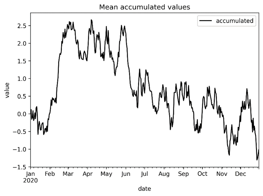
Figure 10.1 - Plot of accumulated means over time
- Save this dataset into a new NetCDF file using the to_netcdf method:
data_array.to_netcdf("data.nc") - Now, we can load the newly created NetCDF file using the load_dataset routine from xarray:
new_data = xr.load_dataset("data.nc")print(new_data)
The output of the preceding code is as follows:
<xarray.Dataset>
Dimensions: (date: 365, location: 25)
Coordinates:
            * location (location) int64 0 1 2 3 4 5 6 7 8 ... 17 18 19 20 21 22 23 24
            * date (date) datetime64[ns] 2020-01-01 2020-01-02 ... 2020-12-30
Data variables:
            steps (date, location) float64 -1.424 1.264 ... -0.4547 -0.4873
            accumulated (date, location) float64 -1.424 1.264 -0.8707 ... 8.935 -3.525
The output shows that the loaded array contains all of the data that we added in the earlier steps. The important steps are 5 and 6, where we store and load this "data.nc" data.
How it works...
The xarray package provides the DataArray and DataSet classes, which are (roughly speaking) multi-dimensional equivalents of the Pandas Series and DataFrame objects. We’re using a dataset in this example because each index – a tuple of a date and location – has two pieces of data associated with it. Both of these objects expose a similar interface to their Pandas equivalents. For example, we can compute the mean along one of the axes using the mean method. The DataArray and DataSet objects also have a convenience method for converting into a Pandas DataFrame called to_dataframe. We used it in this recipe to convert the accumulated column from the means Dataset into a DataFrame for plotting, which isn’t really necessary because xarray has plotting features built into it.
The real focus of this recipe is on the to_netcdf method and the load_dataset routine. The former stores a DataSet object in a NetCDF format file. This requires the netCDF4 package to be installed, as it allows us to access the relevant C library for decoding NetCDF-formatted files. The load_dataset routine is a general-purpose routine for loading data into a DataSet object from various file formats, including NetCDF (again, this requires the netCDF4 package to be installed).
There’s more...
The xarray package has support for a number of data formats in addition to NetCDF, such as OPeNDAP, Pickle, GRIB, and other formats that are supported by Pandas.
Working with geographical data
Many applications involve working with geographical data. For example, when tracking global weather, we might want to plot the temperature as measured by various sensors around the world at their position on a map. For this, we can use the GeoPandas package and the Geoplot package, both of which allow us to manipulate, analyze, and visualize geographical data.
In this recipe, we will use the GeoPandas and Geoplot packages to load and visualize some sample geographical data.
Getting ready
For this recipe, we will need the GeoPandas package, the Geoplot package, and the Matplotlib pyplot package imported as plt:
import geopandas
import geoplot
import matplotlib.pyplot as plt
How to do it...
Follow these steps to create a simple plot of the capital cities plotted on a map of the world using sample data:
- First, we need to load the sample data from the GeoPandas package, which contains the world geometry information:
world = geopandas.read_file(
geopandas.datasets.get_path("naturalearth_lowres"))
- Next, we need to load the data containing the name and position of each of the capital cities of the world:
cities = geopandas.read_file(
geopandas.datasets.get_path("naturalearth_cities"))
- Now, we can create a new figure and plot the outline of the world geometry using the polyplot routine:
fig, ax = plt.subplots()
geoplot.polyplot(world, ax=ax, alpha=0.7)
- Finally, we use the pointplot routine to add the positions of the capital cities on top of the world map. We also set the axes limits to make the whole world visible:
geoplot.pointplot(cities, ax=ax, fc="k", marker="2")
ax.axis((-180, 180, -90, 90))
The resulting plot of the positions of the capital cities of the world looks as follows:

Figure 10.2 - Plot of the world’s capital cities on a map
The plot shows a rough outline of the different countries of the world. Each of the capital cities is indicated by a marker. From this view, it is quite difficult to distinguish individual cities in central Europe.
How it works...
The GeoPandas package is an extension of Pandas that works with geographical data, while the Geoplot package is an extension of Matplotlib that’s used to plot geographical data. The GeoPandas package comes with a selection of sample datasets that we used in this recipe. naturalearth_lowres contains geometric figures that describe the boundaries of countries in the world. This data is not very high-resolution, as signified by its name, which means that some of the finer details of geographical features might not be present on the map (some small islands are not shown at all). naturalearth_cities contains the names and locations of the capital cities of the world. We’re using the datasets.get_path routine to retrieve the path for these datasets in the package data directory. The read_file routine imports the data into the Python session.
The Geoplot package provides some additional plotting routines specifically for plotting geographical data. The polyplot routine plots polygonal data from a GeoPandas DataFrame, which might describe the geographical boundaries of a country. The pointplot routine plots discrete points on a set of axes from a GeoPandas DataFrame, which, in this case, describe the positions of capital cities.
Executing a Jupyter notebook as a script
Jupyter notebooks are a popular medium for writing Python code for scientific and data-based applications. A Jupyter notebook is really a sequence of blocks that is stored in a file in JavaScript Object Notation (JSON) with the ipynb extension. Each block can be one of several different types, such as code or markdown. These notebooks are typically accessed through a web application that interprets the blocks and executes the code in a background kernel that then returns the results to the web application. This is great if you are working on a personal PC, but what if you want to run the code contained within a notebook remotely on a server? In this case, it might not even be possible to access the web interface provided by the Jupyter Notebook software. The papermill package allows us to parameterize and execute notebooks from the command line.
In this recipe, we’ll learn how to execute a Jupyter notebook from the command line using papermill.
Getting ready
For this recipe, we will need to have the papermill package installed, and also have a sample Jupyter notebook in the current directory. We will use the sample.ipynb notebook file stored in the code repository for this chapter.
How to do it...
Follow these steps to use the papermill command-line interface to execute a Jupyter notebook remotely:
- First, we open the sample notebook, sample.ipynb, from the code repository for this chapter. The notebook contains three code cells that hold the following code:
import matplotlib.pyplot as plt
from numpy.random import default_rng
rng = default_rng(12345)
uniform_data = rng.uniform(-5, 5, size=(2, 100))
fig, ax = plt.subplots(tight_layout=True)
ax.scatter(uniform_data[0, :], uniform_data[1, :])
ax.set(title="Scatter plot", xlabel="x", ylabel="y")
- Next, we open the folder containing the Jupyter notebook in the terminal and use the following command:
papermill --kernel python3 sample.ipynb output.ipynb
- Now, we open the output file, output.ipynb, which should now contain the notebook that’s been updated with the result of the executed code. The scatter plot that’s generated in the final block is shown here:
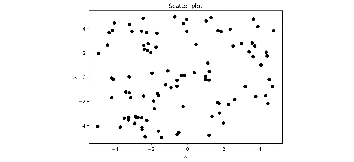
Figure 10.3 - Scatter plot of the random data that was generated inside a Jupyter notebook
Notice that the output of the papermill command is an entirely new notebook that copies the code and text content from the original and is populated with the output of running commands. This is useful for “freezing” the exact code that was used to generate the results.
How it works...
The papermill package provides a simple command-line interface that interprets and then executes a Jupyter notebook and stores the results in a new notebook file. In this recipe, we gave the first argument – the input notebook file – sample.ipynb, and the second argument – the output notebook file – output.ipynb. The tool then executes the code contained in the notebook and produces the output. The notebook’s file format keeps track of the results of the last run, so these results are added to the output notebook and stored at the desired location. In this recipe, this is a simple local file, but papermill can also store them in a cloud location such as Amazon Web Services (AWS) S3 storage or Azure data storage.
In step 2, we added the --kernel python3 option when using the papermill command-line interface. This option allows us to specify the kernel that is used to execute the Jupyter notebook. This might be necessary to prevent errors if papermill tries to execute the notebook with a kernel other than the one used to write the notebook. A list of available kernels can be found by using the following command in the terminal:
jupyter kernelspec list
If you get an error when executing a notebook, you could try changing to a different kernel.
There’s more...
Papermill also has a Python interface so that you can execute notebooks from within a Python application. This might be useful for building web applications that need to be able to perform long-running calculations on external hardware and where the results need to be stored in the cloud. It also has the ability to provide parameters to a notebook. To do this, we need to create a block in the notebook marked with the parameters tag with the default values. Updated parameters can then be provided through the command-line interface using the -p flag, followed by the name of the argument and the value.
Validating data
Data is often presented in a raw form and might contain anomalies or incorrect or malformed data, which will obviously present a problem for later processing and analysis. It is usually a good idea to build a validation step into a processing pipeline. Fortunately, the Cerberus package provides a lightweight and easy-to-use validation tool for Python.
For validation, we have to define a schema, which is a technical description of what the data should look like and the checks that should be performed on the data. For example, we can check the type and place bounds on the maximum and minimum values. Cerberus validators can also perform type conversions during the validation step, which allows us to plug data loaded directly from CSV files into the validator.
In this recipe, we will learn how to use Cerberus to validate data loaded from a CSV file.
Getting ready
For this recipe, we need to import the csv module from the Python Standard Library (https://docs.python.org/3/library/csv.html), as well as the Cerberus package:
import csv
import cerberus
We will also need the sample.csv file from the code repository (https://github.com/PacktPublishing/Applying-Math-with-Python/tree/master/Chapter%2010) for this chapter.
How to do it...
In the following steps, we will validate a set of data that’s been loaded from CSV using the Cerberus package:
- First, we need to build a schema that describes the data we expect. To do this, we must define a simple schema for floating-point numbers:
float_schema = {"type": "float", "coerce": float,"min": -1.0, "max": 1.0}
- Next, we build the schema for individual items. These will be the rows of our data:
item_schema = {"type": "dict",
"schema": {"id": {"type": "string"},"number": {"type": "integer","coerce": int},
"lower": float_schema,
"upper": float_schema,
}
}
- Now, we can define the schema for the whole document, which will contain a list of items:
schema = {"rows": {"type": "list",
"schema": item_schema
}
}
- Next, we create a Validator object with the schema we just defined:
validator = cerberus.Validator(schema)
- Then, we load the data using a DictReader from the csv module:
with open("sample.csv") as f:dr = csv.DictReader(f)
document = {"rows": list(dr)} - Next, we use the validate method on validator to validate the document:
validator.validate(document)
- Then, we retrieve the errors from the validation process from the validator object:
errors = validator.errors["rows"][0]
- Finally, we can print any error messages that appeared:
for row_n, errs in errors.items():
print(f"row {row_n}: {errs}")
The output of the error messages is as follows:
row 11: [{'lower': ['min value is -1.0']}]
row 18: [{'number': ['must be of integer type',      "field 'number' cannot be coerced: invalid literal for int() with base 10: 'None'"]}]
row 32: [{'upper': ['min value is -1.0']}]
row 63: [{'lower': ['max value is 1.0']}]
This has identified four rows that do not conform to the schema that we set out, which limits the float values in “lower” and “upper” to those between -1.0 and 1.0.
How it works...
The schema that we created is a technical description of all the criteria that we need to check our data against. This will usually be defined as a dictionary with the name of the item as the key and a dictionary of properties, such as the type or bounds on the value in a dictionary, as the value. For example, in step 1, we defined a schema for floating-point numbers that limits the numbers so that they’re between the values of -1 and 1. Note that we include the coerce key, which specifies the type that the value should be converted into during the validation. This allows us to pass in data that’s been loaded from a CSV document, which only contains strings, without having to worry about its type.
The validator object takes care of parsing documents so that they’re validated and checking the data they contain against all the criteria described by the schema. In this recipe, we provided the schema to the validator object when it was created. However, we could also pass the schema into the validate method as a second argument. The errors are stored in a nested dictionary that mirrors the structure of the document.
Accelerating code with Cython
Python is often criticized for being a slow programming language – an endlessly debatable statement. Many of these criticisms can be addressed by using a high-performance compiled library with a Python interface – such as the scientific Python stack – to greatly improve performance. However, there are some situations where it is difficult to avoid the fact that Python is not a compiled language. One way to improve performance in these (fairly rare) situations is to write a C extension (or even rewrite the code entirely in C) to speed up the critical parts. This will certainly make the code run more quickly, but it might make it more difficult to maintain the package. Instead, we can use Cython, which is an extension of the Python language that is transpiled into C and compiled for great performance improvements.
For example, we can consider some code that’s used to generate an image of the Mandelbrot set. For comparison, the pure Python code – which we assume is our starting point – is as follows:
# mandelbrot/python_mandel.py
import numpy as np
def in_mandel(cx, cy, max_iter):
    x = cx
    y = cy
    for i in range(max_iter):
        x2 = x**2
        y2 = y**2
        if (x2 + y2) >= 4:
            return i
        y = 2.0*x*y + cy
        x = x2 - y2 + cx
    return max_iter
def compute_mandel(N_x, N_y, N_iter):
    xlim_l = -2.5
    xlim_u = 0.5
    ylim_l = -1.2
    ylim_u = 1.2
    x_vals = np.linspace(xlim_l, xlim_u,
        N_x, dtype=np.float64)
y_vals = np.linspace(ylim_l, ylim_u,
        N_y, dtype=np.float64)
    height = np.empty((N_x, N_y), dtype=np.int64)
    for i in range(N_x):
        for j in range(N_y):
        height[i, j] = in_mandel(
		    x_vals[i], y_vals[j], N_iter)
    return height
The reason why this code is relatively slow in pure Python is fairly obvious: the nested loops. For demonstration purposes, let’s assume that we can’t vectorize this code using NumPy. A little preliminary testing shows that using these functions to generate the Mandelbrot set using 320 × 240 points and 255 steps takes approximately 6.3 seconds. Your times may vary, depending on your system.
In this recipe, we will use Cython to greatly improve the performance of the preceding code in order to generate an image of the Mandelbrot set.
Getting ready
For this recipe, we will need the NumPy package and the Cython package to be installed. You will also need a C compiler such as the GCC installed on your system. For example, on Windows, you can obtain a version of the GCC by installing MinGW.
How to do it...
Follow these steps to use Cython to greatly improve the performance of the code for generating an image of the Mandelbrot set:
- Start a new file called cython_mandel.pyx in the mandelbrot folder. In this file, we will add some simple imports and type definitions:
# mandelbrot/cython_mandel.pyx
import numpy as np
cimport numpy as np
cimport cython
ctypedef Py_ssize_t Int
ctypedef np.float64_t Double
- Next, we define a new version of the in_mandel routine using the Cython syntax. We add some declarations to the first few lines of this routine:
cdef int in_mandel(Double cx, Double cy, int max_iter):
cdef Double x = cx
cdef Double y = cy
cdef Double x2, y2
cdef Int i
- The rest of the function is identical to the Python version of the function:
for i in range(max_iter):
x2 = x**2
y2 = y**2
if (x2 + y2) >= 4:
return i
y = 2.0*x*y + cy
x = x2 - y2 + cx
return max_iter
- Next, we define a new version of the compute_mandel function. We add two decorators to this function from the Cython package:
@cython.boundscheck(False)
@cython.wraparound(False)
def compute_mandel(int N_x, int N_y, int N_iter):
- Then, we define the constants, just as we did in the original routine:
cdef double xlim_l = -2.5
cdef double xlim_u = 0.5
cdef double ylim_l = -1.2
cdef double ylim_u = 1.2
- We use the linspace and empty routines from the NumPy package in exactly the same way as in the Python version. The only addition here is that we declare the i and j variables, which are of the Int type:
cdef np.ndarray x_vals = np.linspace(xlim_l,
xlim_u, N_x, dtype=np.float64)
cdef np.ndarray y_vals = np.linspace(ylim_l,
ylim_u, N_y, dtype=np.float64)
cdef np.ndarray height = np.empty(
(N_x, N_y),dtype=np.int64)
cdef Int i, j
- The remainder of the definition is exactly the same as in the Python version:
for i in range(N_x):
for j in range(N_y):
height[i, j] = in_mandel(
xx_vals[i], y_vals[j], N_iter)
return height
- Next, we create a new file called setup.py in the mandelbrot folder and add the following imports to the top of this file:
# mandelbrot/setup.py
import numpy as np
from setuptools import setup, Extension
from Cython.Build import cythonize
- After that, we define an extension module with the source pointing to the original python_mandel.py file. Set the name of this module to hybrid_mandel:
hybrid = Extension(
"hybrid_mandel",
sources=["python_mandel.py"],
include_dirs=[np.get_include()],
define_macros=[("NPY_NO_DEPRECATED_API","NPY_1_7_API_VERSION")]
)
- Now, we define a second extension module with the source set as the cython_mandel.pyx file that we just created:
cython = Extension(
"cython_mandel",
sources=["cython_mandel.pyx"],
include_dirs=[np.get_include()],
define_macros=[("NPY_NO_DEPRECATED_API","NPY_1_7_API_VERSION")]
)
- Next, we add both these extension modules to a list and call the setup routine to register these modules:
extensions = [hybrid, cython]
setup(
ext_modules = cythonize(
extensions, compiler_directives={"language_level": "3"}),
)
- Create a new empty file called __init__.py in the mandelbrot folder to make this into a package that can be imported into Python.
- Open the terminal inside the mandelbrot folder and use the following command to build the Cython extension modules:
python3.8 setup.py build_ext --inplace
- Now, start a new file called run.py and add the following import statements:
# run.py
from time import time
from functools import wraps
import matplotlib.pyplot as plt
- Import the various compute_mandel routines from each of the modules we have defined: python_mandel for the original; hybrid_mandel for the Cythonized Python code; and cython_mandel for the compiled pure Cython code:
from mandelbrot.python_mandel import compute_mandel
as compute_mandel_py
from mandelbrot.hybrid_mandel import compute_mandel
as compute_mandel_hy
from mandelbrot.cython_mandel import compute_mandel
as compute_mandel_cy
- Define a simple timer decorator that we will use to test the performance of the routines:
def timer(func, name):
@wraps(func)
def wrapper(*args, **kwargs):
t_start = time()
val = func(*args, **kwargs)
t_end = time()
print(f"Time taken for {name}:{t_end - t_start}")return val
return wrapper
- Apply the timer decorator to each of the imported routines, and define some constants for testing:
mandel_py = timer(compute_mandel_py, "Python")
mandel_hy = timer(compute_mandel_hy, "Hybrid")
mandel_cy = timer(compute_mandel_cy, "Cython")
Nx = 320
Ny = 240
steps = 255
- Run each of the decorated routines with the constants we set previously. Record the output of the final call (the Cython version) in the vals variable:
mandel_py(Nx, Ny, steps)
mandel_hy(Nx, Ny, steps)
vals = mandel_cy(Nx, Ny, steps)
- Finally, plot the output of the Cython version to check that the routine computes the Mandelbrot set correctly:
fig, ax = plt.subplots()
ax.imshow(vals.T, extent=(-2.5, 0.5, -1.2, 1.2))
plt.show()
Running the run.py file will print the execution time of each of the routines to the terminal, as follows:
Time taken for Python: 11.399756908416748
Time taken for Hybrid: 10.955225229263306
Time taken for Cython: 0.24534869194030762
Note
These timings are not as good as in the first edition, which is likely due to the way Python is installed on the author’s PC. Your timings may vary.
The plot of the Mandelbrot set can be seen in the following figure:

Figure 10.4 - Image of the Mandelbrot set computed using Cython code
This is what we expect for the Mandelbrot set. Some of the finer detail is visible around the boundary.
How it works...
There is a lot happening in this recipe, so let’s start by explaining the overall process. Cython takes code that is written in an extension of the Python language and compiles it into C code, which is then used to produce a C extension library that can be imported into a Python session. In fact, you can even use Cython to compile ordinary Python code directly to an extension, although the results are not as good as when using the modified language. The first few steps in this recipe define the new version of the Python code in the modified language (saved as a .pyx file), which includes type information in addition to the regular Python code. In order to build the C extension using Cython, we need to define a setup file, and then we create a file that we run to produce the results.
The final compiled version of the Cython code runs considerably faster than its Python equivalent. The Cython-compiled Python code (hybrid, as we called it in this recipe) performs slightly better than the pure Python code. This is because the produced Cython code still has to work with Python objects with all of their caveats. By adding the typing information to the Python code, in the .pyx file, we start to see major improvements in performance. This is because the in_mandel function is now effectively defined as a C-level function that has no interaction with Python objects, and instead operates on primitive data types.
There are some small, but very important differences, between the Cython code and the Python equivalent. In step 1, you can see that we imported the NumPy package as usual but that we also used the cimport keyword to bring some C-level definitions into the scope. In step 2, we used the cdef keyword instead of the def keyword when we defined the in_mandel routine. This means that the in_mandel routine is defined as a C-level function that cannot be used from the Python level, which saves a significant amount of overhead when calling this function (which happens a lot).
The only other real differences regarding the definition of this function are the inclusion of some type declarations in the signature and the first few lines of the function. The two decorators we applied here disable the checking of bounds when accessing elements from a list (array). The boundscheck decorator disables checking whether the index is valid (between 0 and the size of the array), while the wraparound decorator disables the negative indexing. Both of these give a modest improvement to speed during execution, although they disable some of the safety features built into Python. In this recipe, it is OK to disable these checks because we are using a loop over the valid indices of the array.
The setup file is where we tell Python (and therefore Cython) how to build the C extension. The cythonize routine from Cython is the key here, as it triggers the Cython build process. In steps 9 and 10, we defined extension modules using the Extension class from setuptools so that we could define some extra details for the build; specifically, we set an environment variable for the NumPy compilation and added the include files for the NumPy C headers. This is done via the define_macros keyword argument for the Extension class. The terminal command we used in step 13 uses setuptools to build the Cython extensions, and the addition of the --inplace flat means that the compiled libraries will be added to the current directory, rather than being placed in a centralized location. This is good for development.
The run script is fairly simple: import the routines from each of the defined modules – two of these are actually C extension modules – and time their execution. We have to be a little creative with the import aliases and routine names to avoid collisions.
There’s more...
Cython is a powerful tool for improving the performance of some aspects of your code. However, you must always be careful to spend your time wisely while optimizing code. Using a profile such as cProfile that is provided in the Python Standard Library can be used to find the places where performance bottlenecks occur in your code. In this recipe, it was fairly obvious where the performance bottleneck was occurring. Cython is a good remedy to the problem in this case because it involves repetitive calls to a function inside a (double) for loop. However, it is not a universal fix for performance issues and, more often than not, the performance of code can be greatly improved by refactoring it so that it makes use of high-performance libraries.
Cython is well integrated with Jupyter Notebook and can be used seamlessly in the code blocks of a notebook. Cython is also included in the Anaconda distribution of Python, so no additional setup is required for using Cython with Jupyter notebooks when it’s been installed using the Anaconda distribution.
There are alternatives to Cython when it comes to producing compiled code from Python. For example, the Numba package (http://numba.pydata.org/) provides a Just-in-Time (JIT) compiler that optimizes Python code at runtime by simply placing a decorator on specific functions. Numba is designed to work with NumPy and other scientific Python libraries and can also be used to leverage GPUs to accelerate code.
There is also a general-purpose JIT compiler for Python available through the pyjion package (https://www.trypyjion.com/). This can be used in a variety of situations, unlike the Numba library, which is primarily for numerical code. The jax library discussed in Chapter 3 also has a JIT compiler built in, but this too is limited to numerical code.
Distributing computing with Dask
Dask is a library that’s used for distributing computing across multiple threads, processes, or even computers in order to effectively perform computation on a huge scale. This can greatly improve performance and throughput, even if you are working on a single laptop computer. Dask provides replacements for most of the data structures from the Python scientific stack, such as NumPy arrays and Pandas DataFrames. These replacements have very similar interfaces, but under the hood, they are built for distributed computing so that they can be shared between multiple threads, processes, or computers. In many cases, switching to Dask is as simple as changing the import statement, and possibly adding a couple of extra method calls to start concurrent computations.
In this recipe, we will learn how to use Dask to do some simple computations on a DataFrame.
Getting ready
For this recipe, we will need to import the dataframe module from the Dask package. Following the convention set out in the Dask documentation, we will import this module under the dd alias:
import dask.dataframe as dd
We will also need the sample.csv file from the code repository for this chapter.
How to do it...
Follow these steps to use Dask to perform some computations on a DataFrame object:
- First, we need to load the data from sample.csv into a Dask DataFrame. The type of the number column is set to "object" because otherwise, Dask’s type inference will fail (since this column contains None but is otherwise integers):
data = dd.read_csv("sample.csv", dtype={"number":"object"})
- Next, we perform a standard calculation on the columns of the DataFrame:
sum_data = data.lower + data.upper
print(sum_data)
Unlike Pandas DataFrames, the result is not a new DataFrame. The print statement gives us the following information:
Dask Series Structure:
npartitions=1
             float64
                               ...
dtype: float64
Dask Name: add, 4 graph layers
- To actually get the result, we need to use the compute method:
result = sum_data.compute()
print(result.head())
The result is now shown as expected:
0      -0.911811
1       0.947240
2      -0.552153
3      -0.429914
4       1.229118
dtype:  float64
- We compute the means of the final two columns in exactly the same way we would with a Pandas DataFrame, but we need to add a call to the compute method to execute the calculation:
means = data[["lower", "upper"]].mean().compute()
print(means)
The result, as printed, is exactly as we expect it to be:
lower -0.060393
upper -0.035192
dtype: float64
How it works...
Dask builds a task graph for the computation, which describes the relationships between the various operations and calculations that need to be performed on the collection of data. This breaks down the steps of the calculation so that calculations can be done in the right order across the different workers. This task graph is then passed into a scheduler that sends the actual tasks to the workers for execution. Dask comes with several different schedulers: synchronous, threaded, multiprocessing, and distributed. The type of scheduler can be chosen in the call to the compute method or set globally. Dask will choose a sensible default if one is not given.
The synchronous, threaded, and multiprocessing schedulers work on a single machine, while the distributed scheduler is for working with a cluster. Dask allows you to change between schedulers in a relatively transparent way, although for small tasks, you might not get any performance benefits because of the overhead of setting up more complicated schedulers.
The compute method is the key to this recipe. The methods that would ordinarily perform the computation on Pandas DataFrames now just set up a computation that is to be executed through the Dask scheduler. The computation isn’t started until the compute method is called. This is similar to the way that a Future (such as from the asyncio standard library package) is returned as a proxy for the result of an asynchronous function call, which isn’t fulfilled until the computation is complete.
There’s more...
Dask provides interfaces for NumPy arrays, as well as the DataFrames shown in this recipe. There is also a machine learning interface called dask_ml that exposes similar capabilities to the scikit-learn package. Some external packages, such as xarray, also have a Dask interface. Dask can also work with GPUs to further accelerate computations and load data from remote sources, which is useful if the computation is distributed across a cluster.
Writing reproducible code for data science
One of the fundamental principles of the scientific method is the idea that results should be reproducible and independently verifiable. Sadly, this principle is often undervalued in favor of “novel” ideas and results. As practitioners of data science, we have an obligation to do our part to make our analyses and results as reproducible as possible.
Since data science is typically done entirely on computers – that is, it doesn’t usually involve instrumental errors involved in measurements – some might expect that all data science is inherently reproducible. This is certainly not the case. It is easy to overlook simple things such as seeding randomness (see Chapter 3) when using randomized hyperparameter searches or stochastic gradient descent-based optimization. Moreover, more subtle non-deterministic factors (such as use of threading or multiprocessing) can dramatically change results if you are not aware of them.
In this recipe, we’ll look at an example of a basic data analysis pipeline and implement some basic steps to make sure you can reproduce the results.
Getting ready
For this recipe, we will need the NumPy package, imported as np, as usual, the Pandas package, imported as pd, the Matplotlib pyplot interface imported as plt, and the following imports from the scikit-learn package:
from sklearn.metrics import ConfusionMatrixDisplay, accuracy_score
from sklearn.model_selection import train_test_split
from sklearn.tree import DecisionTreeClassifier
We’re going to simulate our data (rather than having to acquire it from elsewhere), so we need to set up an instance of the default random number generator with a seed value (for reproducibility):
rng = np.random.default_rng(12345)
To generate the data, we define the following routine:
def get_data():
	permute = rng.permutation(200)
	data = np.vstack([
		rng.normal((1.0, 2.0, -3.0), 1.0,
		size=(50, 3)),
		rng.normal((-1.0, 1.0, 1.0), 1.0,
		size=(50, 3)),
		rng.normal((0.0, -1.0, -1.0), 1.0,
		size=(50, 3)),
		rng.normal((-1.0, -1.0, -2.0), 1.0,
		size=(50, 3))
		])
	labels = np.hstack(
		[[1]*50, [2]*50, [3]*50,[4]*50])
	X = pd.DataFrame(
		np.take(data, permute, axis=0),
		columns=["A", "B", "C"])
	y = pd.Series(np.take(labels, permute, axis=0))
	return X, y
We’re using this function in place of some other method of loading the data into Python, such as reading from a file or downloading from the internet.
How to do it…
Follow the steps below to create a very simple and reproducible data science pipeline:
- First, we need to “load” our data using the get_data routine we defined previously:
data, labels = get_data()
- Since our data is acquired dynamically, it is a good idea to store the data alongside any results that we generate.
data.to_csv("data.csv")labels.to_csv("labels.csv") - Now, we need to split the data into a training cohort and a testing cohort using the train_test_split routine from scikit-learn. We split the data 80/20 (%) train/test, and make sure the random state is set so this can be repeated (although we will save the indices for reference in the next step):
X_train, X_test, y_train, y_test = train_test_split(
data,labels, test_size=0.2, random_state=23456)
- Now, we make sure that we save the indices of the training and test cohorts so we know precisely which observations were taken in each sample. We can use the indices along with the data stored in step 2 to completely reconstruct the cohorts later:
X_train.index.to_series().to_csv("train_index.csv",index=False, header=False)
X_test.index.to_series().to_csv("test_index.csv",index=False, header=False)
- Now, we can set up and train the classifier. We’re using a simple DecisionTreeClassifier for this example, but this choice is not important. Since the training process involves some randomness, make sure to set the random_state keyword argument to seed this randomness:
classifier = DecisionTreeClassifier(random_state=34567)
classifer.fit(X_train, y_train)
- Before we go any further, it is a good idea to gather some information about the trained model and store it along with the results. The interesting information will vary from model to model. For this model, the feature importance information might be useful, so we record this in a CSV file:
feat_importance = pd.DataFrame(
classifier.feature_importances_,
index=classifier.feature_names_in_,
columns=["Importance"])
feat_importance.to_csv("feature_importance.csv") - Now, we can proceed to check the performance of our model. We’ll evaluate the model on both the training data and the test data, which we will later compare to the true labels:
train_predictions = classifier.predict(X_train)
test_predictions = classifier.predict(X_test)
- Always save the results of this kind of prediction task (or regression, or any other final results that will in some way be part of the report). We convert these into Series objects first to make sure the indices are set correctly:
pd.Series(train_predictions,index=X_train.index,
name="Predicted label").to_csv(
"train_predictions.csv")
pd.Series(test_predictions,index=X_test.index,
name="Predicted label").to_csv(
"test_predictions.csv")
- Finally, we can produce any graphics or metrics that will inform how we proceed with the analysis. Here, we’ll produce a confusion matrix plot for both training and testing cohorts and print out some accuracy summary scores:
fig, (ax1, ax2) = plt.subplots(1, 2, tight_layout=True)
ax1.set_title("Confusion matrix for training data")ax2.set_title("Confusion matrix for test data")ConfusionMatrixDisplay.from_predictions(
y_train, train_predictions,
ax=ax1 cmap="Greys", colorbar=False)
ConfusionMatrixDisplay.from_predictions(
y_test, test_predictions,
ax=ax2 cmap="Greys", colorbar=False)
print(f"Train accuracy {accuracy_score(y_train, train_predictions)}",f"Test accuracy {accuracy_score(y_test, test_predictions)}",sep=" ")
# Train accuracy 1.0
# Test accuracy 0.65
The resulting confusion matrices are shown in Figure 10.5:
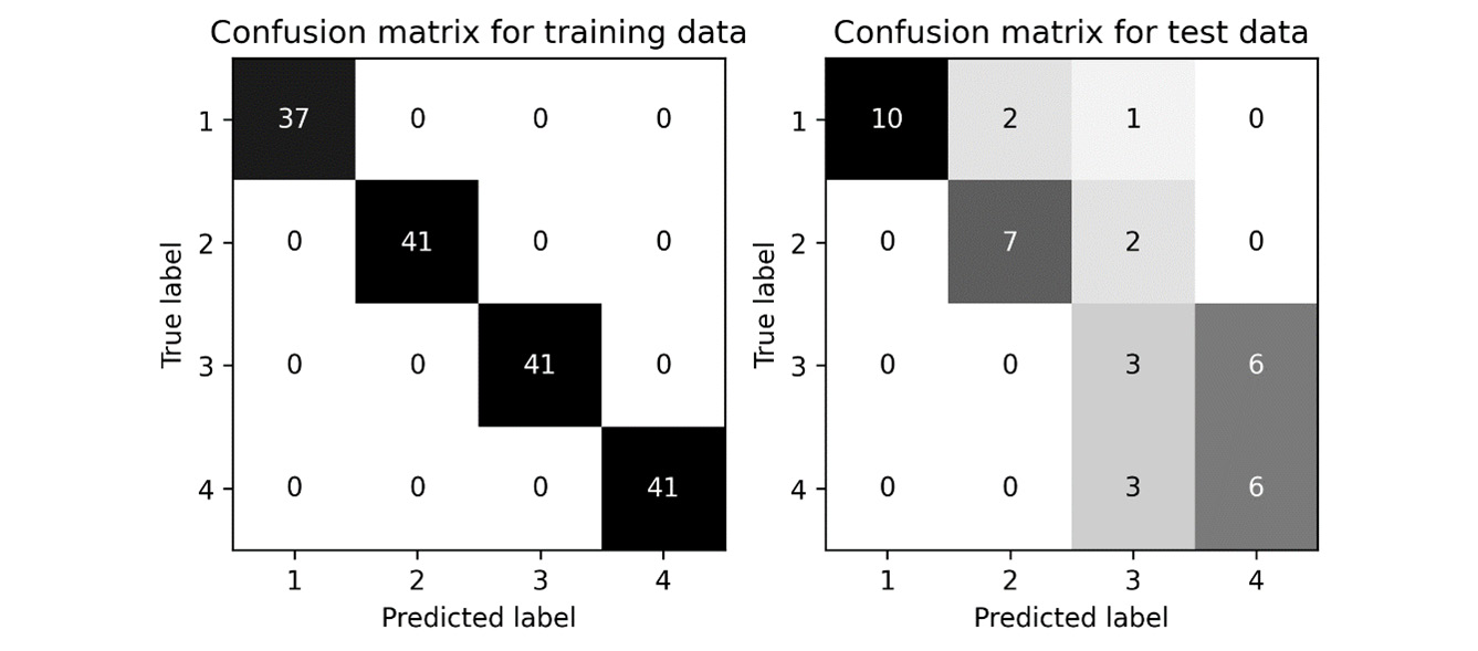
Figure 10.5 - Confusion matrices for a simple classification task
The test results for this example are not spectacular, which should not be a surprise because we spent no time choosing the most appropriate model or tuning, and our sample size was pretty small. Producing an accurate model for this data was not the aim. In the current directory (wherever the script was run), there should be a number of new CSV files containing all the intermediate data we wrote to the disk: data.csv, labels.csv, train_index.csv, test_index.csv, feature_importance.csv, train_predictions.csv, and test_predictions.csv.
How it works…
The are no definitive right answers when it comes to reproducibility, but there are certainly wrong answers. We’ve only touched on a few ideas of how to make your code more reproducible here, but there are many more things one can do. (See There’s more…). In the recipe, we really focused on storing intermediate values and results more than anything else. This is often overlooked in favor of producing plots and graphs – since these are usually the way results will be presented. However, we should not have to rerun the whole pipeline in order to change the styling of a plot. Storing intermediate values allows you to audit various parts of the pipeline and check that what you did was sensible and appropriate and that you can reproduce the results from these intermediate values.
Generally speaking, a data science pipeline will consist of five steps:
- Data acquisition
- Data preprocessing and feature selection
- Model and hyperparameter tuning
- Model training
- Evaluation and results generation
In the recipe, we replaced the data acquisition with a function that randomly generates data. As mentioned in the introduction, this step will usually involve loading data from disk (from CSV files or databases), downloading it from the internet, or gathering it directly from measurement devices. We cached the results of our data acquisition because we are assuming that this is an expensive operation. Of course, this is not always the case; if you load all of the data directly from disk (via a CSV file, for example) then there is obviously no need to store a second copy of this data. However, if you generate the data by querying a large database, then storing a flat copy of the data will dramatically improve the speed at which you can iterate on your pipeline.
Our preprocessing consists only of splitting the data into training and testing cohorts. Again, we store enough data after this step to recreate these cohorts independently later – we stored just the IDs corresponding to each cohort. Since we’re storing these sets, it isn’t totally necessary to seed the randomness in the train_test_split routine, but it is usually a good idea. If your preprocessing involves more intensive operations, then you might consider caching the processed data or the generated features that you will use in the pipeline (we will cover caching in more detail shortly). If your preprocessing step involves selecting features from the columns of your data, then you should absolutely save those selected features to disk alongside the results.
Our model is very simple and doesn’t have any (non-default) hyperparameters. If you have done some hyperparameter tuning, you should store these, along with any other metadata that you might need to reconstruct the model. Storing the model itself (via pickling or otherwise) can be useful but remember that a pickled model might not be readable by another party (for example, if they are using a different version of Python).
You should always store the numerical results from your model. It is impossible to compare plots and other summary figures when you’re checking that your results are the same on subsequent runs. Moreover, this allows you to quickly regenerate figures or values later should this be required. For example, if your analysis involves a binary classification problem, then storing the values used to generate a Receiver Operating Characteristic (ROC) curve is a good idea, even if one also produces a plot of the ROC curve and reports the area under the curve.
There’s more…
There is a lot we have not discussed here. First, let’s address an obvious point. Jupyter notebooks are a common medium for producing data science pipelines. This is fine, but users should understand that this format has several shortcomings. First, and probably most importantly, is the fact that Jupyter notebooks can be run out of order and that later cells might have non-trivial dependencies on earlier cells. To address this, make sure that you always run a notebook on a clean kernel in its entirety, rather than simply rerunning each cell in a current kernel (using tools such as Papermill from the Executing a Jupyter notebook as a script recipe, for example.) Second, the results stored inside the notebook might not correspond to the code that is written in the code cells. This happens when the notebook is run and the code is modified after the fact without a rerun. It might be a good idea to keep a master copy of the notebook without any stored results and make copies of this that are populated with results and are never modified further. Finally, Jupyter notebooks are often executed in environments where it is challenging to properly cache the results of intermediate steps. This is partially addressed by the internal caching mechanism inside the notebook, but this is not always totally transparent.
Let’s address two general concerns of reproducibility now: configuration and caching. Configuration refers to the collection of values that are used to control the setup and execution of the pipeline. We don’t have any obvious configuration values in the recipe except for the random seeds used in the train_test_split routine and the model (and the data generation, but let’s ignore this), and the percentage of values to take in the train/test split. These are hardcoded in the recipe, but this is probably not the best idea. At the very least, we want to be able to record the configuration used in any given run of the analysis. Ideally, the configuration should be loaded (exactly once) from a file and then finalized and cached before the pipeline runs. What this means is that the full configuration is loaded from one or more sources (config files, command-line arguments, or environmental variables), consolidated into a single source of truth, and then serialized into a machine- and human-readable format such as JSON alongside the results. This is so you know precisely what configuration was used to generate the results.
Caching is the process of storing intermediate results so they can be reused later to decrease the running time on subsequent runs. In the recipe, we did store the intermediate results, but we didn’t build the mechanism to reuse the stored data if it exists and is valid. This is because the actual mechanism for checking and loading the cached values is complicated and somewhat dependent on the exact setup. Since our project is very small, it doesn’t necessarily make any sense to cache values. However, for larger projects that have multiple components, this absolutely makes a difference. When implementing a caching mechanism, you should build a system to check whether the cache is valid by, for example, using the SHA-2 hash of the code file and any data sources on which it depends.
When it comes to storing results, it is generally a good idea to store all the results together in a timestamped folder or similar. We don’t do this in the recipe, but it is relatively easy to achieve. For example, using the datetime and pathlib modules from the standard library, we can easily create a base path in which results can be stored:
from pathlib import Path
from datetime import datetime
RESULTS_OUT = Path(datetime.now().isoformat())
...
results.to_csv(RESULTS_OUT / "name.csv")
You must be a little careful if you are using multiprocessing to run multiple analyses in parallel since each new process will generate a new RESULTS_OUT global variable. A better option is to incorporate this into the configuration process, which would also allow the user to customize the output path.
Besides the actual code in the script that we have discussed so far, there is a great deal one can do at the project level to make the code more reproducible. The first, and probably most important step, is to make the code available as far as possible, which includes specifying the license under which the code can be shared (if at all). Moreover, good code will be robust enough that it can be used for analyzing multiple data (obviously, the data should be of the same kind as the data originally used). Also important is making use of version control (Git, Subversion, and so on) to keep track of changes. This also helps distribute the code to other users. Finally, the code needs to be well documented and ideally have automated tests to check that the pipeline works as expected on an example dataset.
See also...
Here are some additional sources of information about reproducible coding practices:
- The Turing Way. Handbook on reproducible, ethical, and collaborative data science produced by the Alan Turing Institute. https://the-turing-way.netlify.app/welcome
- Review criteria for the Journal of Open Source Software: Good practice guidelines to follow with your own code, even if it is not intended to be published: https://joss.readthedocs.io/en/latest/review_criteria.html
This concludes the 10th and final chapter of the book. Remember that we have barely scratched the surface of what is possible when doing mathematics with Python, and you should read the documentation and sources mentioned throughout this book for much more information about what these packages and techniques are capable of.