
4
Working with Randomness and Probability
In this chapter, we will discuss randomness and probability. We will start by briefly exploring the fundamentals of probability by selecting elements from a set of data. Then, we will learn how to generate (pseudo) random numbers using Python and NumPy, and how to generate samples according to a specific probability distribution. We will conclude the chapter by looking at a number of advanced topics covering random processes and Bayesian techniques and using Markov Chain Monte Carlo (MCMC) methods to estimate the parameters of a simple model.
Probability is a quantification of the likelihood of a specific event occurring. We use probabilities intuitively all of the time, although sometimes the formal theory can be quite counterintuitive. Probability theory aims to describe the behavior of random variables whose value is not known, but where the probabilities of the value of this random variable take some (range of) values that are known. These probabilities are usually in the form of one of several probability distributions. Arguably, the most famous probability distribution of this kind is normal distribution, which, for example, can describe the spread of a certain characteristic over a large population.
We will see probability again in a more applied setting in Chapter 6, Working with Data and Statistics, where we will discuss statistics. Here, we will put probability theory to use to quantify errors and build a systematic theory of analyzing data.
In this chapter, we will cover the following recipes:
- Selecting items at random
- Generating random data
- Changing the random number generator
- Generating normally distributed random numbers
- Working with random processes
- Analyzing conversion rates with Bayesian techniques
- Estimating parameters with Monte Carlo simulations
Technical requirements
For this chapter, we require the standard scientific Python packages: NumPy, Matplotlib, and SciPy. We will also require the PyMC package for the final recipe. You can install this using your favorite package manager, such as pip:
python3.10 -m pip install pymc
This command will install the most recent version of PyMC, which, at the time of writing, is 4.0.1. This package provides facilities for probabilistic programming, which involves performing many calculations driven by randomly generated data to understand the likely distribution of a solution to a problem.
Note
In the previous edition, the current version of PyMC was 3.9.2, but since then, PyMC version 4.0 was released and the name reverted to PyMC with this update rather than PyMC3.
The code for this chapter can be found in the Chapter 04 folder of the GitHub repository at https://github.com/PacktPublishing/Applying-Math-with-Python-2nd-Edition/tree/main/Chapter%2004.
Selecting items at random
At the core of probability and randomness is the idea of selecting an item from some kind of collection. As we know, the probability of selecting an item from a collection quantifies the likelihood of that item being selected. Randomness describes the selection of items from a collection according to probabilities without any additional bias. The opposite of a random selection might be described as a deterministic selection. In general, it is very difficult to replicate a purely random process using a computer because computers and their processing are inherently deterministic. However, we can generate sequences of pseudorandom numbers that, when properly constructed, demonstrate a reasonable approximation of randomness.
In this recipe, we will select items from a collection and learn about some of the key terminology associated with probability and randomness that we will need throughout this chapter.
Getting ready
The Python Standard Library contains a module for generating (pseudo) random numbers called random, but in this recipe and throughout this chapter, we will use the NumPy random module instead. The routines in the NumPy random module can be used to generate arrays of random numbers and are slightly more flexible than their standard library counterparts. As usual, we import NumPy under the np alias.
Before we can proceed, we need to fix some terminology. A sample space is a set (a collection with no repeated elements) and an event is a subset of the sample space. The probability that an event, ![]() , occurs is denoted as
, occurs is denoted as ![]() , and is a number between 0 and 1. A probability of 0 indicates that the event can never occur, while a probability of 1 indicates that an event will certainly occur. The probability of the whole sample space must be 1.
, and is a number between 0 and 1. A probability of 0 indicates that the event can never occur, while a probability of 1 indicates that an event will certainly occur. The probability of the whole sample space must be 1.
When the sample space is discrete, then probabilities are just numbers between 0 and 1 associated with each of the elements, where the sum of all these numbers is 1. This gives meaning to the probability of selecting a single item (an event consisting of a single element) from a collection. We will consider methods for selecting items from a discrete collection here and deal with the continuous case in the Generating normally distributed random numbers recipe.
How to do it...
Perform the following steps to select items at random from a container:
- The first step is to set up the random number generator. For the moment, we will use the default random number generator for NumPy, which is recommended in most cases. We can do this by calling the default_rng routine from the NumPy random module, which will return an instance of a random number generator. We will usually call this function without a seed, but for this recipe, we will add a 12345 seed so that our results are repeatable:
rng = np.random.default_rng(12345)
# changing seed for repeatability
- Next, we need to create the data and probabilities that we will select from. This step can be skipped if you already have the data stored or if you want to select elements with equal probabilities:
data = np.arange(15)
probabilities = np.array(
[0.3, 0.2, 0.1, 0.05, 0.05, 0.05, 0.05, 0.025,
0.025, 0.025, 0.025, 0.025, 0.025, 0.025, 0.025]
)
As a quick sanity test, we can use an assertion to check that these probabilities do indeed sum to 1:
assert round(sum(probabilities), 10) == 1.0,
    "Probabilities must sum to 1"
Now, we can use the choice method on the random number generator, rng, to select the samples from data according to the probabilities just created. For this selection, we want to turn the replacement on, so calling the method multiple times can select from the entire data:
selected = rng.choice(data,p=probabilities,replace=True)
# 0
To select multiple items from data, we can also supply the size argument, which specifies the shape of the array to be selected. This plays the same role as the shape keyword argument with many of the other NumPy array creation routines. The argument given to size can be either an integer or a tuple of integers:
selected_array = rng.choice(data, p=probabilities,  replace=True, size=(5, 5))
#array([[ 1, 6, 4, 1, 1],
#         [ 2, 0, 4, 12, 0],
#         [12, 4, 0, 1, 10],
#         [ 4, 1, 5, 0, 0],
#         [ 0, 1, 1, 0, 7]])
We can see that there appear to be more 0s and 1s in the sampled data, for which we assigned probabilities of 0.3 and 0.2 respectively. Interestingly, only one 2 appears, and yet we have two 12s, despite the probability of a 12 appearing being half that of a 2. This is not a problem; a larger probability does not guarantee that individual numbers will appear in a sample, only that we’d expect to see roughly twice as many 2s as 12s in a large number of samples.
How it works...
The default_rng routine creates a new Pseudorandom Number Generator (PRNG) instance (with or without a seed) that can be used to generate random numbers or, as we saw in the recipe, select items at random from predefined data. NumPy also has an implicit state-based interface for generating random numbers using routines directly from the random module. However, it is generally advisable to create the generator explicitly, using default_rng, or create a Generator instance yourself. Being more explicit in this way is more Pythonic and should lead to more reproducible results (in some sense).
A seed is a value that is passed to a random number generator in order to generate the values. The generator generates a sequence of numbers in a completely deterministic way based only on the seed. This means that two instances of the same PRNGs provided with the same seed will generate the same sequence of random numbers. If no seed is provided, the generators typically produce a seed that depends on the user’s system.
The Generator class from NumPy is a wrapper around a low-level pseudorandom bit generator, which is where the random numbers are actually generated. In recent versions of NumPy, the default PRNG algorithm is the 128-bit permuted congruential generator. By contrast, Python’s built-in random module uses a Mersenne Twister PRNG. More information about the different options for PRNG algorithms is given in the Changing the random number generator recipe.
The choice method on a Generator instance performs selections according to random numbers generated by the underlying BitGenerator. The optional p keyword argument specifies the probability associated with each item from the data provided. If this argument isn’t provided, then a uniform probability is assumed, where each item has an equal probability of being selected. The replace keyword argument specifies whether selections should be made with or without a replacement. We turned replacement on so that the same element can be selected more than once. The choice method uses the random numbers given by the generator to make the selections, which means that two PRNGs of the same type using the same seed will select the same items when using the choice method.
This process of choosing points from a bag of possible choices is a good way to think about discrete probability. This is where we assign a certain weight – for example, 1 over the number of points – to each of a finite number of points, where the sum of these weights is 1. Sampling is the process of choosing points at random according to the weights assigned by the probability (we can assign discrete probabilities to infinite sets too, but this is more complicated because of the constraint that the weights must sum to 1 and this is also impractical for computation).
There’s more...
The choice method can also be used to create random samples of a given size by passing replace=False as an argument. This guarantees the selection of distinct items from the data, which is good for generating a random sample. This might be used, for example, to select users to test a new version of an interface from the whole group of users; most sample statistical techniques rely on randomly selected samples.
Generating random data
Many tasks involve generating large quantities of random numbers, which, in their most basic form, are either integers or floating-point numbers (double-precision) lying within the range ![]() . Ideally, these numbers should be selected uniformly, so that if we draw a large number of these numbers, they are distributed roughly evenly across the range
. Ideally, these numbers should be selected uniformly, so that if we draw a large number of these numbers, they are distributed roughly evenly across the range ![]() .
.
In this recipe, we will see how to generate large quantities of random integers and floating-point numbers using NumPy, and show the distribution of these numbers using a histogram.
Getting ready
Before we start, we need to import the default_rng routine from the NumPy random module and create an instance of the default random number generator to use in the recipe:
from numpy.random import default_rng
rng = default_rng(12345) # changing seed for reproducibility
We have discussed this process in the Selecting items at random recipe.
We also import the Matplotlib pyplot module under the plt alias.
How to do it...
Perform the following steps to generate uniform random data and plot a histogram to understand its distribution:
- To generate random floating-point numbers between 0 and 1, including 0 but not 1, we use the random method on the rng object:
random_floats = rng.random(size=(5, 5))
# array([[0.22733602, 0.31675834, 0.79736546, 0.67625467, 0.39110955],
# [0.33281393, 0.59830875, 0.18673419, 0.67275604, 0.94180287],
# [0.24824571, 0.94888115, 0.66723745, 0.09589794, 0.44183967],
# [0.88647992, 0.6974535 , 0.32647286, 0.73392816, 0.22013496],
# [0.08159457, 0.1598956 , 0.34010018, 0.46519315, 0.26642103]])
- To generate random integers, we use the integers method on the rng object. This will return integers in the specified range:
random_ints = rng.integers(1, 20, endpoint=True, size=10)
# array([12, 17, 10, 4, 1, 3, 2, 2, 3, 12])
- To examine the distribution of the random floating-point numbers, we first need to generate a large array of random numbers, just as we did in step 1. While this is not strictly necessary, a larger sample will be able to show the distribution more clearly. We generate these numbers as follows:
dist = rng.random(size=1000)
- To show the distribution of the numbers we have generated, we plot a histogram of the data:
fig, ax = plt.subplots()
ax.hist(dist, color="k", alpha=0.6)
ax.set_title("Histogram of random numbers")ax.set_xlabel("Value")ax.set_ylabel("Density")
The resulting plot is shown in Figure 4.1. As we can see, the data is roughly evenly distributed across the whole range:

Figure 4.1 – Histogram of randomly generated random numbers between 0 and 1
As the number of sampled points increases, we would expect these bars to “even out” and look more and more like the flat line that we expect from a uniform distribution. Compare this to the same histogram with 10,000 random points in Figure 4.2 here:

Figure 4.2 – Histogram of 10,000 uniformly distributed random numbers
We can see here that, although not totally flat, the distribution is much more even across the whole range.
How it works...
The Generator interface provides three simple methods for generating basic random numbers, not including the choice method that we discussed in the Selecting items at random recipe. In addition to the random method for generating random floating-point numbers and the integers method for generating random integers, there is also a bytes method for generating raw random bytes. Each of these methods calls a relevant method on the underlying BitGenerator instance. Each of these methods also enables the data type of the generated numbers to be changed, for example, from double- to single-precision floating-point numbers.
There’s more...
The integers method on the Generator class combines the functionality of the randint and random_integers methods on the old RandomState interface through the addition of the endpoint optional argument (in the old interface, the randint method excluded the upper endpoint, whereas the random_integers method included the upper endpoint). All of the random data generating methods on Generator allow the data type of the data they generate to be customized, which was not possible using the old interface (this interface was introduced in NumPy 1.17).
In Figure 4.1, we can see that the histogram of the data that we generated is approximately uniform over the range ![]() . That is, all of the bars are approximately level (they are not completely level due to the random nature of the data). This is what we expect from uniformly distributed random numbers, such as those generated by the random method. We will explain distributions of random numbers in greater detail in the Generating normally distributed random numbers recipe.
. That is, all of the bars are approximately level (they are not completely level due to the random nature of the data). This is what we expect from uniformly distributed random numbers, such as those generated by the random method. We will explain distributions of random numbers in greater detail in the Generating normally distributed random numbers recipe.
Changing the random number generator
The random module in NumPy provides several alternatives to the default PRNG, which uses a 128-bit permutation congruential generator. While this is a good general-purpose random number generator, it might not be sufficient for your particular needs. For example, this algorithm is very different from the one used in Python’s internal random number generator. We will follow the guidelines for best practice set out in the NumPy documentation for running repeatable but suitably random simulations.
In this recipe, we will show you how to change to an alternative PRNG and how to use seeds effectively in your programs.
Getting ready
As usual, we import NumPy under the np alias. Since we will be using multiple items from the random package, we import that module from NumPy, too, using the following code:
from numpy import random
You will need to select one of the alternative random number generators that are provided by NumPy (or define your own; refer to the There’s more... section in this recipe). For this recipe, we will use the MT19937 random number generator, which uses a Mersenne Twister-based algorithm like the one used in Python’s internal random number generator.
How to do it...
The following steps show how to generate seeds and different random number generators in a reproducible way:
- We will generate a SeedSequence object that can reproducibly generate new seeds from a given source of entropy. We can either provide our own entropy as an integer, very much like how we provide the seed for default_rng, or we can let Python gather entropy from the operating system. We will pick the latter method here to demonstrate its use. For this, we do not provide any additional arguments to create the SeedSequence object:
seed_seq = random.SeedSequence()
- Now that we have the means to generate the seeds for random number generators for the rest of the session, we log the entropy next so that we can reproduce this session later if necessary. The following is an example of what the entropy should look like; your results will inevitably differ somewhat:
print(seed_seq.entropy)
# 9219863422733683567749127389169034574
- Now, we can create the underlying BitGenerator instance that will provide the random numbers for the wrapping Generator object:
bit_gen = random.MT19937(seed_seq)
- Next, we create the wrapping Generator object around this BitGenerator instance to create a usable random number generator:
rng = random.Generator(bit_gen)
Once created, you can use this random number generator as we have seen in any of the previous recipes.
How it works...
As mentioned in the Selecting items at random recipe, the Generator class is a wrapper around an underlying BitGenerator that implements a given pseudorandom number algorithm. NumPy provides several implementations of pseudorandom number algorithms through the various subclasses of the BitGenerator class: PCG64 (default); MT19937 (as seen in this recipe); Philox; and SFC64. These bit generators are implemented in Cython.
The PCG64 generator should provide high-performance random number generation with good statistical quality (this might not be the case on 32-bit systems). The MT19937 generator is slower than more modern PRNGs and does not produce random numbers with good statistical properties. However, this is the random number generator algorithm that is used by the Python Standard Library random module. The Philox generator is relatively slow but produces random numbers of very high quality while the SFC64 generator is fast and of reasonably good quality, but doesn’t have as good statistical properties as other generators.
The SeedSequence object created in this recipe is a means to create seeds for random number generators in an independent and reproducible manner. In particular, this is useful if you need to create independent random number generators for several parallel processes, but still need to be able to reconstruct each session later to debug or inspect results. The entropy stored on this object is a 128-bit integer that was gathered from the operating system and serves as a source of random seeds.
The SeedSequence object allows us to create a separate random number generator for each independent process or thread, which eliminates any data race problems that might make results unpredictable. It also generates seed values that are very different from one another, which can help avoid problems with some PRNGs (such as MT19937, which can produce very similar streams with two similar 32-bit integer seed values). Obviously, having two independent random number generators producing the same or very similar values will be problematic when we are depending on the independence of these values.
There’s more...
The BitGenerator class serves as a common interface for generators of raw random integers. The classes mentioned previously are those that are implemented in NumPy with the BitGenerator interface. You can also create your own BitGenerator subclasses, although this needs to be implemented in Cython.
Note
Refer to the NumPy documentation at https://numpy.org/devdocs/reference/random/extending.html#new-bit-generators for more information.
Generating normally distributed random numbers
In the Generating random data recipe, we generated random floating-point numbers following a uniform distribution between 0 and 1, but not including 1. However, in most cases where we require random data, we need to follow one of several different distributions instead. Roughly speaking, a distribution function is a function, ![]() , that describes the probability that a random variable has a value that is below
, that describes the probability that a random variable has a value that is below ![]() . In practical terms, the distribution describes the spread of the random data over a range. In particular, if we create a histogram of data that follows a particular distribution, then it should roughly resemble the graph of the distribution function. This is best seen by example.
. In practical terms, the distribution describes the spread of the random data over a range. In particular, if we create a histogram of data that follows a particular distribution, then it should roughly resemble the graph of the distribution function. This is best seen by example.
One of the most common distributions is normal distribution, which appears frequently in statistics and forms the basis for many statistical methods that we will see in Chapter 6, Working with Data and Statistics. In this recipe, we will demonstrate how to generate data following normal distribution, and plot a histogram of this data to see the shape of the distribution.
Getting ready
As in the Generating random data recipe, we import the default_rng routine from the NumPy random module and create a Generator instance with a seeded generator for demonstration purposes:
from numpy.random import default_rng
rng = default_rng(12345)
As usual, we import the Matplotlib pyplot module as plt, and NumPy as np.
How to do it...
In the following steps, we generate random data that follows a normal distribution:
- We use the normal method on our Generator instance to generate the random data according to the normal distribution. The normal distribution has two parameters: location and scale. There is also an optional size argument that specifies the shape of the generated data (see the Generating random data recipe for more information on the size argument). We generate an array of 10,000 values to get a reasonably sized sample:
mu = 5.0 # mean value
sigma = 3.0 # standard deviation
rands = rng.normal(loc=mu, scale=sigma, size=10000)
- Next, we plot a histogram of this data. We have increased the number of bins in the histogram. This isn’t strictly necessary, as the default number (10) is perfectly adequate, but it does show the distribution slightly better:
fig, ax = plt.subplots()
ax.hist(rands, bins=20, color="k", alpha=0.6)
ax.set_title("Histogram of normally distributed data")ax.set_xlabel("Value")ax.set_ylabel("Density") - Next, we create a function that will generate the expected density for a range of values. This is given by multiplying the probability density function for normal distribution by the number of samples (10,000):
def normal_dist_curve(x):
return 10000*np.exp(
-0.5*((x-mu)/sigma)**2)/(sigma*np.sqrt(2*np.pi))
- Finally, we plot our expected distribution over the histogram of our data:
x_range = np.linspace(-5, 15)
y = normal_dist_curve(x_range)
ax.plot(x_range, y, "k--")
The result is shown in Figure 4.3. We can see here that the distribution of our sampled data closely follows the expected distribution from a normal distribution curve:

Figure 4.3 – Histogram of data drawn from a normal distribution, with the expected density overlaid
Again, if we took larger and larger samples, we’d expect that the roughness of the sample would begin to smooth out and approach the expected density (shown as the dashed line in Figure 4.3).
How it works...
Normal distribution has a probability density function defined by the following formula:

This is related to the normal distribution function, ![]() , according to the following formula:
, according to the following formula:

This probability density function peaks at the mean value, which coincides with the location parameter, and the width of the bell shape is determined by the scale parameter. We can see in Figure 4.3 that the histogram of the data generated by the normal method on the Generator object fits the expected distribution very closely.
The Generator class uses a 256-step ziggurat method to generate normally distributed random data, which is fast compared to the Box-Muller or inverse CDF implementations that are also available in NumPy.
There’s more...
The normal distribution is one example of a continuous probability distribution, in that it is defined for real numbers and the distribution function is defined by an integral (rather than a sum). An interesting feature of normal distribution (and other continuous probability distributions) is that the probability of selecting any given real number is 0. This is reasonable because it only makes sense to measure the probability that a value selected in this distribution lies within a given range.
Normal distribution is important in statistics, mostly due to the central limit theorem. Roughly speaking, this theorem states that sums of Independent and Identically Distributed (IID) random variables, with a common mean and variance, are eventually like normal distribution with a common mean and variance. This holds, regardless of the actual distribution of these random variables. This allows us to use statistical tests based on normal distribution in many cases even if the actual distribution of the variables is not necessarily normal (we do, however, need to be extremely cautious when appealing to the central limit theorem).
There are many other continuous probability distributions aside from normal distribution. We have already encountered uniform distribution over a range of 0 to 1. More generally, uniform distribution over the range ![]() has a probability density function given by the following equation:
has a probability density function given by the following equation:

Other common examples of continuous probability density functions include exponential distribution, beta distribution, and gamma distribution. Each of these distributions has a corresponding method on the Generator class that generates random data from that distribution. These are typically named according to the name of the distribution, all in lowercase letters, so for the aforementioned distributions, the corresponding methods are exponential, beta, and gamma. These distributions each have one or more parameters, such as location and scale for normal distribution, that determine the final shape of the distribution. You may need to consult the NumPy documentation (https://numpy.org/doc/1.18/reference/random/generator.html#numpy.random.Generator) or other sources to see what parameters are required for each distribution. The NumPy documentation also lists the probability distributions from which random data can be generated.
Working with random processes
In this recipe, we will examine a simple example of a random process that models the number of bus arrivals at a stop over time. This process is called a Poisson process. A Poisson process, ![]() , has a single parameter,
, has a single parameter, ![]() , which is usually called the intensity or rate, and the probability that
, which is usually called the intensity or rate, and the probability that ![]() takes the value
takes the value ![]() at a given time
at a given time ![]() is given by the following formula:
is given by the following formula:

This equation describes the probability that ![]() buses have arrived by time
buses have arrived by time ![]() . Mathematically, this equation means that
. Mathematically, this equation means that ![]() has a Poisson distribution with the parameter
has a Poisson distribution with the parameter ![]() . There is, however, an easy way to construct a Poisson process by taking sums of inter-arrival times that follow an exponential distribution. For instance, let
. There is, however, an easy way to construct a Poisson process by taking sums of inter-arrival times that follow an exponential distribution. For instance, let ![]() be the time between the (
be the time between the (![]() )-st arrival and the
)-st arrival and the ![]() -th arrival, which are exponentially distributed with parameter
-th arrival, which are exponentially distributed with parameter ![]() . Now, we take the following equation:
. Now, we take the following equation:
![]()
Here, the number ![]() is the maximum
is the maximum ![]() such that
such that ![]() . This is the construction that we will work through in this recipe. We will also estimate the intensity of the process by taking the mean of the inter-arrival times.
. This is the construction that we will work through in this recipe. We will also estimate the intensity of the process by taking the mean of the inter-arrival times.
Getting ready
Before we start, we import the default_rng routine from NumPy’s random module and create a new random number generator with a seed for the purpose of demonstration:
from numpy.random import default_rng
rng = default_rng(12345)
In addition to the random number generator, we also import NumPy as np and the Matplotlib pyplot module as plt. We also need to have the SciPy package available.
How to do it...
The following steps show how to model the arrival of buses using a Poisson process:
- Our first task is to create the sample inter-arrival times by sampling data from an exponential distribution. The exponential method on the NumPy Generator class requires a scale parameter, which is
 , where
  is the rate. We choose a rate of 4, and create 50 sample inter-arrival times:
rate = 4.0
inter_arrival_times = rng.exponential(
scale=1./rate, size=50)
- Next, we compute the actual arrival times by using the accumulate method of the NumPy add universal function. We also create an array containing the integers 0 to 49, representing the number of arrivals at each point:
arrivals = np.add.accumulate(inter_arrival_times)
count = np.arange(50)
- Next, we plot the arrivals over time using the step plotting method:
fig1, ax1 = plt.subplots()
ax1.step(arrivals, count, where="post")
ax1.set_xlabel("Time")ax1.set_ylabel("Number of arrivals")ax1.set_title("Arrivals over time")
The result is shown in Figure 4.4, where the length of each horizontal line represents the inter-arrival times:
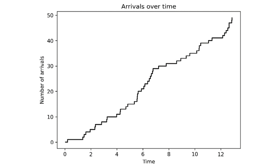
Figure 4.4 – Arrivals over time where inter-arrival times are exponentially distributed
- Next, we define a function that will evaluate the probability distribution of the counts at a time, which we will take as 1 here. This uses the formula for the Poisson distribution that we gave in the introduction to this recipe:
def probability(events, time=1, param=rate):
return ((param*time)**events/factorial(
events))*np.exp(- param*time)
- Now, we plot the probability distribution over the count per unit of time, since we chose time=1 in the previous step. We will add to this plot later:
fig2, ax2 = plt.subplots()
ax2.plot(N, probability(N), "k", label="True distribution")
ax2.set_xlabel("Number of arrivals in 1 time unit")ax2.set_ylabel("Probability")ax2.set_title("Probability distribution") - Now, we move on to estimate the rate from our sample data. We do this by computing the mean of the inter-arrival times, which, for exponential distribution, is an estimator of the scale
 :
:estimated_scale = np.mean(inter_arrival_times)
estimated_rate = 1.0/estimated_scale
- Finally, we plot the probability distribution with this estimated rate for the counts per unit of time. We plot this on top of the true probability distribution that we produced in step 5:
ax2.plot(N, probability(
N, param=estimated_rate),
"k--",label="Estimated distribution")
ax2.legend()
The resulting plot is given in Figure 4.5, where we can see that, apart from a small discrepancy, the estimated distribution is very close to the true distribution:
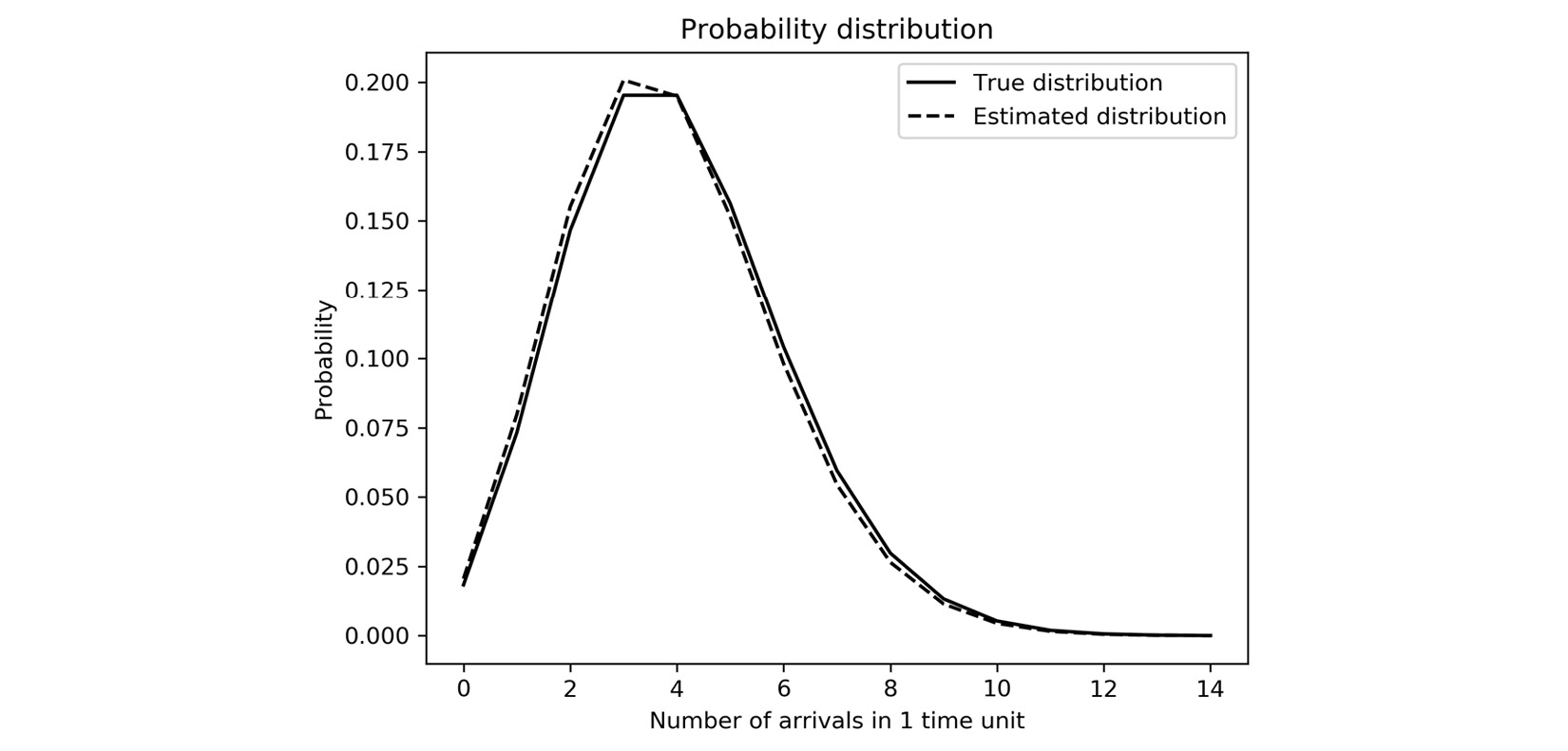
Figure 4.5 – Distribution of the number of arrivals per time unit, estimated and true
The distribution shown in Figure 4.5 follows the Poisson distribution as described in the introduction to this recipe. You can see that moderate numbers of arrivals per unit of time are more likely than large numbers. The most likely counts are determined by the rate parameter ![]() , which is 4.0 in this example.
, which is 4.0 in this example.
How it works...
Random processes exist everywhere. Roughly speaking, a random process is a system of related random variables, usually indexed with respect to time ![]() for a continuous random process, or by natural numbers
for a continuous random process, or by natural numbers ![]() for a discrete random process. Many (discrete) random processes satisfy the Markov property, which makes them a Markov chain. The Markov property is the statement that the process is memoryless, in that only the current value is important for the probabilities of the next value.
for a discrete random process. Many (discrete) random processes satisfy the Markov property, which makes them a Markov chain. The Markov property is the statement that the process is memoryless, in that only the current value is important for the probabilities of the next value.
A Poisson process is a counting process that counts the number of events (bus arrivals) that occur in an amount of time if the events are randomly spaced (in time) with an exponential distribution with a fixed parameter. We constructed the Poisson process by sampling inter-arrival times from exponential distribution, following the construction we described in the introduction. However, it turns out that this fact (that the inter-arrival times are exponentially distributed) is a property of all Poisson processes when they are given their formal definition in terms of probabilities.
In this recipe, we sampled 50 points from an exponential distribution with a given rate parameter. We had to do a small conversion because the NumPy Generator method for sampling from an exponential distribution uses a related scale parameter, which is 1 over the rate parameter. Once we have these points, we create an array that contains cumulative sums of these exponentially distributed numbers. This creates our arrival times. The actual Poisson process is the one displayed in Figure 4.4 and is a combination of the arrival times with the corresponding number of events that have occurred at that time.
The mean (expected value) of an exponential distribution coincides with the scale parameter, so the mean of a sample drawn from an exponential distribution is one way to estimate the scale (rate) parameter. This estimate will not be perfect since our sample is relatively small. This is why there is a small discrepancy between the two plots in Figure 4.5.
There’s more...
There are many types of random processes describing a wide variety of real-world scenarios. In this recipe, we modeled arrival times using a Poisson process. A Poisson process is a continuous random process, meaning that it is parameterized by a continuous variable, ![]() , rather than a discrete variable,
, rather than a discrete variable, ![]() . Poisson processes are actually Markov chains, under a suitably generalized definition of a Markov chain, and also an example of a renewal process. A renewal process is a process that describes the number of events that occur within a period of time. The Poisson process described here is an example of a renewal process.
. Poisson processes are actually Markov chains, under a suitably generalized definition of a Markov chain, and also an example of a renewal process. A renewal process is a process that describes the number of events that occur within a period of time. The Poisson process described here is an example of a renewal process.
Many Markov chains also satisfy some properties in addition to their defining Markov property. For example, a Markov chain is homogeneous if the following equality holds for all ![]() ,
, ![]() , and
, and ![]() values:
values:
![]()
In simple terms, this means that the probabilities of moving from one state to another over a single step do not change as we increase the number of steps. This is extremely useful for examining the long-term behavior of a Markov chain.
It is very easy to construct simple examples of homogeneous Markov chains. Suppose that we have two states, ![]() and
and ![]() . At any given step, we could be either at state
. At any given step, we could be either at state ![]() or state
or state ![]() . We move between states according to a certain probability. For instance, let’s say that the probability of transitioning from state
. We move between states according to a certain probability. For instance, let’s say that the probability of transitioning from state ![]() to state
to state ![]() is 0.4 and the probability of transitioning from
is 0.4 and the probability of transitioning from ![]() to
to ![]() is 0.6. Similarly, let’s say that the probability of transitioning from
is 0.6. Similarly, let’s say that the probability of transitioning from ![]() to
to ![]() is 0.2, and transitioning from
is 0.2, and transitioning from ![]() to
to ![]() is 0.8. Notice that both the probability of switching and the probability of staying the same sum 1 in both cases. We can represent the probability of transitioning from each state in matrix form given, in this case, with the following equation:
is 0.8. Notice that both the probability of switching and the probability of staying the same sum 1 in both cases. We can represent the probability of transitioning from each state in matrix form given, in this case, with the following equation:

This matrix is called the transition matrix. The idea here is that the probability of being in a particular state after a step is given by multiplying the vector containing the probability of being in state ![]() and
and ![]() (position 0 and 1, respectively). For example, if we start in state
(position 0 and 1, respectively). For example, if we start in state ![]() , then the probability vector will contain a 1 at index 0 and 0 at index 1. Then, the probability of being in state
, then the probability vector will contain a 1 at index 0 and 0 at index 1. Then, the probability of being in state ![]() after 1 step is given by 0.4, and the probability of being in state
after 1 step is given by 0.4, and the probability of being in state ![]() is 0.6. This is what we expect given the probabilities we outlined previously. However, we could also write this calculation using the matrix formula:
is 0.6. This is what we expect given the probabilities we outlined previously. However, we could also write this calculation using the matrix formula:

To get the probability of being in either state after two steps, we multiply the right-hand side vector again by the transition matrix, ![]() , to obtain the following:
, to obtain the following:

We can continue this process ad infinitum to obtain a sequence of state vectors, which constitute our Markov chain. This construction can be applied, with more states if necessary, to model many simple, real-world problems.
Analyzing conversion rates with Bayesian techniques
Bayesian probability allows us to systematically update our understanding (in a probabilistic sense) of a situation by considering data. In more technical language, we update the prior distribution (our current understanding) using data to obtain a posterior distribution. This is particularly useful, for example, when examining the proportion of users who go on to buy a product after viewing a website. We start with our prior belief distribution. For this, we will use the beta distribution, which models the probability of success given a number of observed successes (completed purchases) against failures (no purchases). For this recipe, we will assume that our prior belief is that we expect 25 successes from 100 views (75 fails). This means that our prior belief follows a beta (25, 75) distribution. Let’s say that we wish to calculate the probability that the true rate of success is at least 33%.
Our method is roughly divided into three steps. First, we need to understand our prior belief for the conversion rate, which we have decided follows a beta (25, 75) distribution. We compute the probability that the conversion rate is at least 33% by integrating (numerically) the probability density function for the prior distribution from 0.33 to 1. The next step is to apply Bayesian reasoning to update our prior belief with new information. Then, we can perform the same integration with the posterior (updated) belief to examine the probability that the conversion rate is at least 33% given this new information.
In this recipe, we will see how to use Bayesian techniques to update a prior belief based on new information for our hypothetical website.
Getting ready
As usual, we will need the NumPy and Matplotlib packages imported as np and plt, respectively. We will also require the SciPy package, imported as sp.
How to do it...
The following steps show how to estimate and update conversion rate estimations using Bayesian reasoning:
- The first step is to set up the prior distribution. For this, we use the beta distribution object from the SciPy stats module, which has various methods for working with beta distribution. We import the beta distribution object from the stats module under a beta_dist alias and then create a convenience function for the probability density function:
from scipy.stats import beta as beta_dist
beta_pdf = beta_dist.pdf
- Next, we need to compute the probability, under the prior belief distribution, that the success rate is at least 33%. To do this, we use the quad routine from the SciPy integrate module, which performs numerical integration of a function. We use this to integrate the probability density function for the beta distribution, imported in step 1, with our prior parameters. We print the probability according to our prior distribution to the console:
prior_alpha = 25
prior_beta = 75
args = (prior_alpha, prior_beta)
prior_over_33, err = sp.integrate.quad(
beta_pdf, 0.33, 1, args=args)
print("Prior probability", prior_over_33)# 0.037830787030165056
- Now, suppose we have received some information about successes and failures over a new period of time. For example, we observed 122 successes and 257 failures over this period. We create new variables to reflect these values:
observed_successes = 122
observed_failures = 257
- To obtain the parameter values for the posterior distribution with a beta distribution, we simply add the observed successes and failures to the prior_alpha and prior_beta parameters, respectively:
posterior_alpha = prior_alpha + observed_successes
posterior_beta = prior_beta + observed_failures
- Now, we repeat our numerical integration to compute the probability that the success rate is now above 33% using the posterior distribution (with our new parameters computed earlier). Again, we print this probability to the terminal:
args = (posterior_alpha, posterior_beta)
posterior_over_33, err2 = sp.integrate.quad(
beta_pdf, 0.33, 1, args=args)
print("Posterior probability", posterior_over_33)# 0.13686193416281017
- We can see here that the new probability, given the updated posterior distribution, is 14% as opposed to the prior 4%. This is a significant difference, although we are still not confident that the conversion rate is above 33% given these values. Now, we plot the prior and posterior distribution to visualize this increase in probability. To start with, we create an array of values and evaluate our probability density function based on these values:
p = np.linspace(0, 1, 500)
prior_dist = beta_pdf(p, prior_alpha, prior_beta)
posterior_dist = beta_pdf(
p, posterior_alpha, posterior_beta)
- Finally, we plot the two probability density functions computed in step 6 onto a new plot:
fig, ax = plt.subplots()
ax.plot(p, prior_dist, "k--", label="Prior")
ax.plot(p, posterior_dist, "k", label="Posterior")
ax.legend()
ax.set_xlabel("Success rate")ax.set_ylabel("Density")ax.set_title("Prior and posterior distributions for success rate")
The resulting plot is shown in Figure 4.6, where we can see that the posterior distribution is much more narrow and centered to the right of the prior:

Figure 4.6 – Prior and posterior distributions of a success rate following a beta distribution
We can see that the posterior distribution peaks at around 0.3, but most of the mass of the distribution lies close to this peak.
How it works...
Bayesian techniques work by taking a prior belief (probability distribution) and using Bayes’ theorem to combine the prior belief with the likelihood of our data given this prior belief to form a posterior (updated) belief. This is similar to how we might understand things in real life. For example, when you wake up on a given day, you might have the belief (from a forecast or otherwise) that there is a 40% chance of rain outside. Upon opening the blinds, you see that it is very cloudy outside, which might indicate that rain is more likely, so we update our belief according to this new data to say a 70% chance of rain.
To understand how this works, we need to understand conditional probability. Conditional probability deals with the probability that one event will occur given that another event has already occurred. In symbols, the probability of event ![]() given that event
given that event ![]() has occurred is written as follows:
has occurred is written as follows:
![]()
Bayes’ theorem is a powerful tool that can be written (symbolically) as follows:

The probability ![]() represents our prior belief. The event
represents our prior belief. The event ![]() represents the data that we have gathered, so that
represents the data that we have gathered, so that ![]() is the likelihood that our data arose given our prior belief. The probability
is the likelihood that our data arose given our prior belief. The probability ![]() represents the probability that our data arose, and
represents the probability that our data arose, and ![]() represents our posterior belief given the data. In practice, the probability
represents our posterior belief given the data. In practice, the probability ![]() can be difficult to calculate or otherwise estimate, so it is quite common to replace the strong equality above with a proportional version of Bayes’ theorem:
can be difficult to calculate or otherwise estimate, so it is quite common to replace the strong equality above with a proportional version of Bayes’ theorem:
![]()
In the recipe, we assumed that our prior belief was beta-distributed. The beta distribution has a probability density function given by the following equation:

Here, ![]() is the gamma function. The likelihood is binomially distributed, which has a probability density function given by the following equation:
is the gamma function. The likelihood is binomially distributed, which has a probability density function given by the following equation:

Here, ![]() is the number of observations, and
is the number of observations, and ![]() is one of those that were successful. In the recipe, we observed
is one of those that were successful. In the recipe, we observed ![]() successes and
successes and ![]() failures, which gives
failures, which gives ![]() and
and ![]() . To calculate the posterior distribution, we can use the fact that the beta distribution is a conjugate prior for the binomial distribution to see that the right-hand side of the proportional form of Bayes’ theorem is beta-distributed with parameters of
. To calculate the posterior distribution, we can use the fact that the beta distribution is a conjugate prior for the binomial distribution to see that the right-hand side of the proportional form of Bayes’ theorem is beta-distributed with parameters of ![]() and
and ![]() . This is what we used in the recipe. The fact that the beta distribution is a conjugate prior for binomial random variables makes them useful in Bayesian statistics.
. This is what we used in the recipe. The fact that the beta distribution is a conjugate prior for binomial random variables makes them useful in Bayesian statistics.
The method we demonstrated in this recipe is a rather basic example of using a Bayesian method, but it is still useful for updating our prior beliefs when systematically given new data.
There’s more...
Bayesian methods can be used for a wide variety of tasks, making it a powerful tool. In this recipe, we used a Bayesian approach to model the success rate of a website based on our prior belief of how it performs and additional data gathered from users. This is a rather complex example since we modeled our prior belief on a beta distribution. Here is another example of using Bayes’ theorem to examine two competing hypotheses using only simple probabilities (numbers between 0 and 1).
Suppose you place your keys in the same place every day when you return home, but one morning you wake up to find that they are not in this place. After searching for a short time, you cannot find them and so conclude that they must have vanished from existence. Let’s call this hypothesis ![]() . Now,
. Now, ![]() certainly explains the data,
certainly explains the data, ![]() , that you cannot find your keys – hence, the likelihood
, that you cannot find your keys – hence, the likelihood ![]() (if your keys vanished from existence, then you could not possibly find them). An alternative hypothesis is that you simply placed them somewhere else when you got home the night before. Let’s call this hypothesis
(if your keys vanished from existence, then you could not possibly find them). An alternative hypothesis is that you simply placed them somewhere else when you got home the night before. Let’s call this hypothesis ![]() . Now, this hypothesis also explains the data, so
. Now, this hypothesis also explains the data, so ![]() , but in reality,
, but in reality, ![]() is far more plausible than
is far more plausible than ![]() . Let’s say that the probability that your keys completely vanished from existence is 1 in 1 million – this is a huge overestimation, but we need to keep the numbers reasonable – while you estimate that the probability that you placed them elsewhere the night before is 1 in 100. Computing the posterior probabilities, we have the following:
. Let’s say that the probability that your keys completely vanished from existence is 1 in 1 million – this is a huge overestimation, but we need to keep the numbers reasonable – while you estimate that the probability that you placed them elsewhere the night before is 1 in 100. Computing the posterior probabilities, we have the following:

This highlights the reality that it is 10,000 times more likely that you simply misplaced your keys as opposed to the fact that they simply vanished. Sure enough, you soon find your keys already in your pocket because you had picked them up earlier that morning.
Estimating parameters with Monte Carlo simulations
Monte Carlo methods broadly describe techniques that use random sampling to solve problems. These techniques are especially powerful when the underlying problem involves some kind of uncertainty. The general method involves performing large numbers of simulations, each sampling different inputs according to a given probability distribution, and then aggregating the results to give a better approximation of the true solution than any individual sample solution.
MCMC is a specific kind of Monte Carlo simulation in which we construct a Markov chain of successively better approximations of the true distribution that we seek. This works by accepting or rejecting a proposed state, sampled at random, based on carefully selected acceptance probabilities at each stage, with the aim of constructing a Markov chain whose unique stationary distribution is precisely the unknown distribution that we wish to find.
In this recipe, we will use the PyMC package and MCMC methods to estimate the parameters of a simple model. The package will deal with most of the technical details of running simulations, so we don’t need to go any further into the details of how the different MCMC algorithms actually work.
Getting ready
As usual, we import the NumPy package and Matplotlib pyplot module as np and plt, respectively. We also import and create a default random number generator, with a seed for the purpose of demonstration, as follows:
from numpy.random import default_rng
rng = default_rng(12345)
We will also need a module from the SciPy package for this recipe as well as the PyMC package, which is a package for probabilistic programming. We import the PyMC package under the pm alias:
import pymc as pm
Let’s see how to use the PyMC package to estimate the parameters of a model given an observed, noisy sample.
How to do it...
Perform the following steps to use MCMC simulations to estimate the parameters of a simple model using sample data:
- Our first task is to create a function that represents the underlying structure that we wish to identify. In this case, we will be estimating the coefficients of a quadratic (a polynomial of degree 2). This function takes two arguments, which are the points in the range, which is fixed, and the variable parameters that we wish to estimate:
def underlying(x, params):
return params[0]*x**2 + params[1]*x + params[2]
- Next, we set up the true parameters and a size parameter that will determine how many points are in the sample that we generate:
size = 100
true_params = [2, -7, 6]
- We generate the sample that we will use to estimate the parameters. This will consist of the underlying data, generated by the underlying function we defined in step 1, plus some random noise that follows a normal distribution. We first generate a range of
 values, which will stay constant throughout the recipe, and then use the underlying function and the normal method on our random number generator to generate the sample data:
x_vals = np.linspace(-5, 5, size)
raw_model = underlying(x_vals, true_params)
noise = rng.normal(loc=0.0, scale=10.0, size=size)
sample = raw_model + noise
- It is a good idea to plot the sample data, with the underlying data overlaid, before we begin the analysis. We use the scatter plotting method to plot only the data points (without connecting lines), and then plot the underlying quadratic structure using a dashed line:
fig1, ax1 = plt.subplots()
ax1.scatter(x_vals, sample,
label="Sampled data", color="k",
alpha=0.6)
ax1.plot(x_vals, raw_model,
"k--", label="Underlying model")
ax1.set_title("Sampled data")ax1.set_xlabel("x")ax1.set_ylabel("y")
The result is Figure 4.7, where we can see that the shape of the underlying model is still visible even with the noise, although the exact parameters of this model are no longer obvious:

Figure 4.7 – Sampled data with the underlying model overlaid
- The basic object of PyMC programming is the Model class, which is usually created using the context manager interface. We also create our prior distributions for the parameters. In this case, we will assume that our prior parameters are normally distributed with a mean of 1 and a standard deviation of 1. We need three parameters, so we provide the shape argument. The Normal class creates random variables that will be used in the Monte Carlo simulations:
with pm.Model() as model:
params = pm.Normal(
"params", mu=1, sigma=1, shape=3)
- We create a model for the underlying data, which can be done by passing the random variable, param, that we created in step 6 into the underlying function that we defined in step 1. We also create a variable that handles our observations. For this, we use the Normal class since we know that our noise is normally distributed around the underlying data, y. We set a standard deviation of 2 and pass our observed sample data into the observed keyword argument (this is also inside the Model context):
y = underlying(x_vals, params)
y_obs = pm.Normal("y_obs",mu=y, sigma=2, observed=sample)
- To run the simulations, we need only call the sample routine inside the Model context. We pass the cores argument to speed up the calculations, but leave all of the other arguments as the default values:
trace = pm.sample(cores=4)
These simulations should take a short time to execute.
- Next, we plot the posterior distributions that use the plot_posterior routine from PyMC. This routine takes the trace result from the sampling step that performed the simulations. We create our own figures and axes using the plt.subplots routine in advance, but this isn’t strictly necessary. We are using three subplots on a single figure, and we pass the axs2 tuple of Axes to the plotting routing under the ax keyword argument:
fig2, axs2 = plt.subplots(1, 3, tight_layout=True)
pm.plot_posterior(trace, ax=axs2, color="k")
The resulting plot is shown in Figure 4.8, where you can see that each of these distributions is approximately normal, with a mean that is similar to the true parameter values:
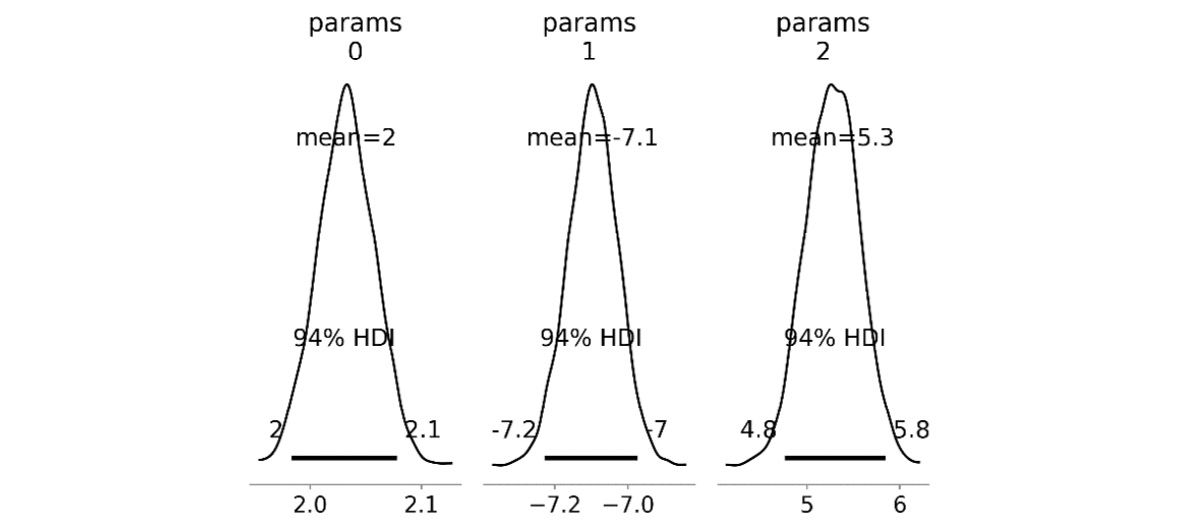
Figure 4.8 – Posterior distributions of estimated parameters
- Now, retrieve the mean of each of the estimated parameters from the trace result. We access the estimated parameters from the posterior attribute on trace and then use the mean method on the params item (with axes=(0,1) to average over all chains and all samples) and convert this into a NumPy array. We print these estimated parameters in the terminal:
estimated_params = trace.posterior["params"].mean(
axis=(0, 1)). to_numpy()
print("Estimated parameters", estimated_params)# Estimated parameters [ 2.03220667 -7.09727509 5.27548983]
- Finally, we use our estimated parameters to generate our estimated underlying data by passing the
 values and the estimated parameters to the underlying function defined in step 1. We then plot this estimated underlying data together with the true underlying data on the same axes:
estimated = underlying(x_vals, estimated_params)
fig3, ax3 = plt.subplots()
ax3.plot(x_vals, raw_model, "k", label="True model")
ax3.plot(x_vals, estimated, "k--", label="Estimated model")
ax3.set_title("Plot of true and estimated models")ax3.set_xlabel("x")ax3.set_ylabel("y")ax3.legend()
The resulting plot is in Figure 4.9, where there is only a small difference between these two models in this range:

Figure 4.9 – True model and estimated model plotted on the same axes
In Figure 4.9 we can see that there is a small discrepancy between the true model and the estimated model.
How it works...
The interesting part of the code in this recipe can be found in the Model context manager. This object keeps track of the random variables, orchestrates the simulations, and keeps track of the state. The context manager gives us a convenient way to separate the probabilistic variables from the surrounding code.
We start by proposing a prior distribution for the distribution of the random variables representing our parameters, of which there are three. We proposed a normal distribution since we know that the parameters cannot stray too far from the value 1 (we can tell this by looking at the plot that we generated in step 4, for example). Using a normal distribution will give a higher probability to the values that are close to the current values. Next, we add the details relating to the observed data, which is used to calculate the acceptance probabilities that are used to either accept or reject a state. Finally, we start the sampler using the sample routine. This constructs the Markov chain and generates all of the step data.
The sample routine sets up the sampler based on the types of variables that will be simulated. Since the normal distribution is a continuous variable, the sample routine selected the No U-turn Sampler (NUTS). This is a reasonable general-purpose sampler for continuous variables. A common alternative to the NUTS is the Metropolis sampler, which is less reliable but faster than the NUTS in some cases. The PyMC documentation recommends using the NUTS whenever possible.
Once the sampling is complete, we plotted the posterior distribution of the trace (the states given by the Markov chain) to see the final shape of the approximations we generated. We can see here that all three of our random variables (parameters) are normally distributed around approximately the correct value.
Under the hood, PyMC uses Aesara – the successor to Theano used by PyMC3 – to speed up its calculations. This makes it possible for PyMC to perform computations on a Graphics Processing Unit (GPU) rather than on the Central Processing Unit (CPU) for a considerable boost to computation speed.
There’s more...
The Monte Carlo method is very flexible and the example we gave here is one particular case where it can be used. A more typical basic example of where the Monte Carlo method is applied is for estimating the value of integrals – commonly, Monte Carlo integration. A really interesting case of Monte Carlo integration is estimating the value of ![]() . Let’s briefly look at how this works.
. Let’s briefly look at how this works.
First, we take the unit disk, whose radius is 1 and therefore has an area of ![]() . We can enclose this disk inside a square with vertices at the points
. We can enclose this disk inside a square with vertices at the points ![]() ,
, ![]() ,
, ![]() , and
, and ![]() . This square has an area of 4 since the edge length is 2. Now, we can generate random points uniformly over this square. When we do this, the probability that any one of these random points lies inside a given region is proportional to the area of that region. Thus, the area of a region can be estimated by multiplying the proportion of randomly generated points that lie within the region by the total area of the square. In particular, we can estimate the area of the disk (when the radius is 1, this is
. This square has an area of 4 since the edge length is 2. Now, we can generate random points uniformly over this square. When we do this, the probability that any one of these random points lies inside a given region is proportional to the area of that region. Thus, the area of a region can be estimated by multiplying the proportion of randomly generated points that lie within the region by the total area of the square. In particular, we can estimate the area of the disk (when the radius is 1, this is ![]() ) by simply multiplying the number of randomly generate points that lie within the disk by 4 and dividing by the total number of points we generated.
) by simply multiplying the number of randomly generate points that lie within the disk by 4 and dividing by the total number of points we generated.
We can easily write a function in Python that performs this calculation, which might be the following:
import numpy as np
from numpy.random import default_rng
def estimate_pi(n_points=10000):
    rng = default_rng()
    points = rng.uniform(-1, 1, size=(2, n_points))
    inside = np.less(points[0, :]**2 + points[1, :]**2, 1)
    return 4.0*inside.sum() / n_points
Running this function just once will give a reasonable approximation of π:
estimate_pi() # 3.14224
We can improve the accuracy of our estimation by using more points, but we could also run this a number of times and average the results. Let’s run this simulation 100 times and average the results (we’ll use concurrent futures to parallelize this so that we can run larger numbers of samples if we want):
from statistics import mean
results = list(estimate_pi() for _ in  range(100))
print(mean(results))
Running this code once prints the estimated value of ![]() as 3.1415752, which is an even better estimate of the true value.
as 3.1415752, which is an even better estimate of the true value.
See also
The PyMC package has many features that are documented by numerous examples (https://docs.pymc.io/). There is also another probabilistic programming library based on TensorFlow (https://www.tensorflow.org/probability).
Further reading
A good, comprehensive reference for probability and random processes is the following book:
- Grimmett, G. and Stirzaker, D. (2009). Probability and random processes. 3rd ed. Oxford: Oxford Univ. Press.
An easy introduction to Bayes’ theorem and Bayesian statistics is the following:
- Kurt, W. (2019). Bayesian statistics the fun way. San Francisco, CA: No Starch Press, Inc.