
7
Aggregation
In Chapter 6, Multi-Document ACID Transactions, we worked through two use cases of new transactional capabilities using the code for Ruby and Python. In this chapter, we will dive deeper into the aggregation framework, learning how it can be useful. Additionally, we will look at the aggregation operators that are supported by MongoDB.
Following that, we will learn about the time series collections, which were introduced in version 5 and greatly expanded in version 6. Next, we will learn about MongoDB views, which are similar to traditional database materialized views.
Finally, we will discuss the most major aggregation pipeline limitations and bring everything together with a sample aggregation use case.
To learn this information, we will use aggregations to process transaction data from the Ethereum blockchain. The complete source code is available at https://github.com/PacktPublishing/Mastering-MongoDB-6.x.
In this chapter, we will cover the following topics:
- Why aggregation?
- Aggregation options
- Different aggregation operators
- Time series collections
- MongoDB views
- Aggregation limitations
- Optimizing aggregation pipelines
- An aggregation use case
Technical requirements
To follow the examples in this chapter, we will need to install MongoDB, the official PyMongo Python driver v.4.1, and import the data files from chapter 7 of the book’s GitHub repository.
Why aggregation?
The aggregation framework was introduced by MongoDB in version 2.2 (version 2.1 in the development branch). It serves as an alternative to both the MapReduce framework, which is deprecated as of version 5.0, and querying the database directly.
Using the aggregation framework, we can perform GROUP BY operations in the server. Therefore, we can project only the fields that are needed in the result set. Using the $match and $project operators, we can reduce the amount of data passed through the pipeline, resulting in faster data processing.
Self-joins—that is, joining data within the same collection—can also be performed using the aggregation framework, as we will see in our use case.
When comparing the aggregation framework to simply using the queries available via the shell or various other drivers, it is important to remember that there is a use case for both.
For selection and projection queries, it’s almost always better to use simple queries, as the complexity of developing, testing, and deploying an aggregation framework operation cannot easily outweigh the simplicity of using built-in commands. Finding documents with ( db.books.find({price: 50} {price: 1, name: 1}) ), or without ( db.books.find({price: 50}) ) projecting only some of the fields, is simple and fast enough to not warrant the usage of the aggregation framework.
On the other hand, if we want to perform GROUP BY and self-join operations using MongoDB, there might be a case for using the aggregation framework. The most important limitation of the group() command in the MongoDB shell is that the resulting set has to fit in a document, meaning that it can’t be more than 16 MB in size. In addition, the result of any group() command can’t have more than 20,000 results.
Finally, there is always the option of using the database as data storage and performing complex operations using the application. Sometimes, this can be quick to develop but should be avoided, as it will most likely incur memory, networking, and ultimately performance costs down the road.
In the next section, we will describe the available operators before using them in a real use case.
Aggregation options
Usually, the use case for aggregation is grouping together attribute values from multiple documents or returning a single result after processing a set of documents.
We can also use the aggregation framework to track how data changes over time in a collection.
One example would be calculating the average value for an attribute across all documents of a collection.
We can use either one or more aggregation pipelines, forming a Directed Acyclic Graph (DAG) for the calculations or a single-purpose aggregation method for simple one-off calculations.
In earlier versions, we could also use Map Reduce, but as of MongoDB 5.0, the Map-reduce framework has been deprecated and, as such, should not be used for new development.
Existing map reduce code can be rewritten using an aggregation pipeline in multiple stages. The $accumulator and $function aggregator operators that were introduced in MongoDB 4.4 can be used to define custom aggregation expressions using JavaScript. This should be useful in the somewhat specific case where our mapper and reducer contain custom code that cannot be expressed using an aggregation pipeline. Writing custom code opens up the possibility of code injection vulnerabilities, and this should be weighed as a security risk.
Single-purpose aggregation methods
MongoDB provides three helper aggregation methods that can be used directly from the shell or official drivers to avoid writing code where we want to perform count or distinct operations.
They are estimatedDocumentCount(), count(), and distinct():
- count() is a method wrapper for a combined $group and $sum aggregation pipeline and, as such, will provide an accurate count of documents at all times.
- distinct() will, similarly, perform a distinct count, which can include query or collation options.
- estimatedDocumentCount() uses internal MongoDB metadata collection statistics to return a quick estimation of the total number of documents in the collection. It cannot filter based on a query. For example, in the case of an unclean shutdown using the default WiredTiger storage engine, it will return the latest count calculated at the last checkpoint before the shutdown occurred. By default, the checkpoint frequency is 60 seconds. Custom syncdelay set at the server level can also affect the delta in seconds between the latest checkpoint and the shutdown.
Finally, using estimatedDocumentCount() in sharded clusters might not filter out orphaned documents.
Note
The estimatedDocumentCount() method refers to the new mongo shell, mongosh. There might be identical method names in Node.js or other language drivers. Check the documentation, and use the guideline that the older the library is, the greater the odds are that the method is referring to a different definition of estimated count than the previously mentioned calculation that mongosh and compatible drivers use as of MongoDB 5.
Single-purpose aggregation methods can be used as helper methods but should not be, generally, used as a replacement. In the next section, we will learn about the more advanced aggregation operators using pipelines and the recommended usage by MongoDB.
Aggregation operators
In this section, we will learn how to use aggregation operators. Aggregation operators are divided into two categories. Within each stage, we use expression operators to compare and process values. Between different stages, we use aggregation stage operators to define the data that will get passed on from one stage to the next, as it is considered to be in the same format.
Aggregation pipeline stages
An aggregation pipeline is composed of different stages. These stages are declared in an array and executed sequentially, with the output of every stage being the input of the next one.
The last stage of the pipeline has to be either an $out operator or a $merge operator.
The $out stage has to be the final stage in an aggregation pipeline, outputting data to an output collection that will be completely erased and overwritten if it already exists. The $out operator cannot output to a sharded collection.
Additionally, the $merge stage has to be the final stage in an aggregation pipeline, but it can insert, merge, replace, or keep existing documents. It can also process the documents using a custom update pipeline. It can replace all the documents in a collection but only if the aggregation results output matches all of the existing documents in the collection. The $merge operator can also output to a sharded collection.
At most, the $out and $merge (and $geoNear) stages can only appear once in an aggregation pipeline.
The following list describes the most important aggregation pipeline stages:
- $addFields: This adds new fields to documents and outputs the same number of documents as input with the added fields.
- $bucket: This splits the documents into buckets based on predefined selection criteria and bucket boundaries.
- $bucketAuto: This splits documents into buckets based on predefined selection criteria and attempts to evenly distribute documents among the buckets.
- $collStats: This returns statistics regarding the view or collection.
- $count: This returns a count of the number of documents at this stage of the pipeline.
- $densify: This will create new documents and fill in the gaps in a sequence of documents where the values in the specified field are missing.
- $documents: This will return literal documents from our input values. It can be used for testing or to inject documents into the pipeline programmatically.
- $facet: This combines multiple aggregation pipelines within a single stage.
- $fill: This will populate null and missing field values within the specified documents. We can use the linear regression or Last Observation Carried Forward (locf) methods to generate the values.
- $geoNear: This returns an ordered list of documents based on the proximity to a specified field. The output documents include a computed distance field.
- $graphLookup: This recursively searches a collection and adds an array field with the results of the search in each output document.
- $group: This is most commonly used to group by identifier expression and to apply the accumulator expression. It outputs one document per distinct group.
- $indexStats: This returns statistics regarding the indexes of the collection.
- $limit: This limits the number of documents passed on to the next aggregation phase based on predefined criteria.
- $listSessions: This is only available as the first step in the pipeline. It will list active sessions by querying the system.sessions collection. All sessions are initiated in memory local to each node before MongoDB syncs them with the system.sessions collection. We can list in-memory sessions using the $ listLocalSessions operation in the node.
- $lookup: This is used for filtering documents from the input. The input could be documents from another collection in the same database selected by an outer left join or the literal $documents from the input values operator.
- $match: This is used for filtering documents from input based on criteria.
- $merge
- $out: This outputs the documents from this pipeline stage to an output collection by replacing or adding to the documents that already exist in the collection.
- $project: This is used for document transformation, and outputs one document per input document.
- $redact: As a combination of $project and $match, this will redact the selected fields from each document and pass them on to the next stage of the pipeline.
- $replaceRoot: This replaces all existing fields of the input document (including the standard _id field) with the specified fields.
- $replaceWith: This will replace a document with the specified embedded document. The operation replaces all of the existing fields in the input document, including the _id field. Specify a document embedded in the input document to promote the embedded document to the top level. $replaceWith is an alias for the $replaceRoot stage.
- $sample: This randomly selects a specified number of documents from the input.
- $search: This is used to perform a full-text search in the input-specified fields. It can return a snippet of the text including the search term. It can only be the first step in the pipeline; MongoDB Atlas only.
- $searchMeta: MongoDB Atlas only. This is not available in self-hosted clusters.
- $set: This will add new fields to the specified documents. $set will reformat each document passing through the stream and may add new fields to the output documents with both the existing fields and the new ones. It is an alias of the $addFields stage.
- $setWindowFields: This will group input documents into partitions (windows) and apply our operators to all documents in each partition.
- $skip: This skips a certain number of documents, preventing them from passing on to the next stage of the pipeline.
- $sort: This sorts the documents based on criteria.
- $sortByCount: This groups incoming documents based on the value of an expression and computes the count of documents in each bucket.
- $unionWith: This will perform a union of two collections to merge the results from two collections into one result set. It is similar to SQL’s UNION ALL operator.
- $unset: This will remove fields from the output documents. $unset is an alias for the $project stage that removes fields.
- $unwind: This transforms an array of n elements into n documents, mapping each document to one element of the array. The documents are then passed on to the next stage of the pipeline.
Aggregation pipeline expression operators
Within every stage, we can define one or more expression operators to apply our intermediate calculations. This section will focus on these expression operators.
Expression Boolean operators
The Boolean operators are used to pass a true or false value to the next stage of our aggregation pipeline.
We can choose to pass the originating integer, string, or any other type value along, too.
We can use the $and, $or, and $not operators in the same way that we would use them in any programming language.
Note
A Boolean expression will evaluate as false any null, 0, or undefined values.
Expression comparison operators
Comparison operators can be used in conjunction with Boolean operators to construct the expressions that we need to evaluate as true/false for the output of our pipeline’s stage.
The most commonly used operators are listed as follows:
- $cmp
- $eq ( equal )
- $gt (greater than)
- $gte (greater than or equal)
- $lt
- $lte
- $ne ( not equal)
All of these previously mentioned operators return a Boolean value of true or false.
The only operator that doesn’t return a Boolean value is $cmp, which returns 0 if the two arguments are equivalent, 1 if the first value is greater than the second, and -1 if the second value is greater than the first.
Set expression and array operators
As with most programming languages, set operations ignore duplicate entries and the order of elements, treating them as sets. The order of results is unspecified, and duplicates will be deduplicated in the result set. Set expressions do not apply recursively to elements of the set, but only to the top level. This means that if a set contains, for example, a nested array, then this array may or may not contain duplicates.
The available set operators are listed as follows:
- $allElementsTrue: This is true if all of the elements in the set evaluate to true.
- $anyElementTrue: This is true if any of the elements in the set evaluate to true.
- $setDifference: This returns the documents that appear in the first input set but not the second.
- $setEquals: This is true if the two sets have the same distinct elements.
- $setIntersection: This returns the intersection of all input sets (that is, the documents that appear in all of the input sets).
- $setIsSubset: This is true if all documents in the first set appear in the second one, even if the two sets are identical.
- $setUnion: This returns the union of all input sets (that is, the documents that appear in at least one of all of the input sets).
The available array operators are listed as follows:
- $arrayElemAt: This is used to retrieve the element at the array index position, starting from zero.
- $arrayToObject: This is used to transform an array into a document.
- $concatArrays: This returns a concatenated array.
- $filter: This returns a subset of the array based on specified criteria.
- $first: This will return the first element of the array. Note that this is different from the $first accumulator operator.
- $firstN: This will return the first N elements of the array. Note that this is different from the $first accumulator operator.
- $in: This returns true if the specified value is in the array; otherwise, it returns false.
- $indexOfArray: This returns the index of the array that fulfills the search criteria. If it does not exist, then it will return -1.
- $isArray: This returns true if the input is an array; otherwise, it returns false.
- $last: This returns the last element of the array. Note that this is different from the $last accumulator operator.
- $lastN: This returns the last N elements of the array. Note that this is different from the $lastN accumulator operator.
- $map: This is similar to JavaScript and the map() function of other languages. This operator will apply the expression to each element of the array and return an array of the resulting values in order. It accepts named parameters.
- $maxN: This returns the largest N values of the array. Note that this is different from the $maxN accumulator operator.
- $minN: This returns the smallest N values of the array. Note that this is different from the $minN accumulator operator.
- $objectToArray: This operator will convert a document into an array of documents representing key-value pairs.
- $range: This outputs an array containing a sequence of integers according to user-defined inputs.
- $reduce: This reduces the elements of an array to a single value according to the specified input.
- $reverseArray: This returns an array with the elements in reverse order.
- $size: This returns the number of items in the array.
- $slice: This returns a subset of the array.
- $sortArray: This operator sorts the elements of the array. The array can contain simple values, where we can define 1 for ascending and –1 for descending order. Or it can contain documents, where we can define the field to sort by the order direction in the same way.
- $zip: This returns a merged array.
Expression date operators
The date operators are used to extract date information from date fields when we want to calculate statistics based on the day of the week, month, or year using the pipeline:
- $dateAdd: This is used to add a number of time units to a date object.
- $dateDiff: This is used to get the delta difference between two dates in the defined unit (year, month, and second).
- $dateFromParts: This constructs a date object from a set of fields. It can be either year/month-millisecond or an isoWeekDate format with year/week/dayOfWeek… /millisecond format.
- $dateFromString: This converts a string into a date object according to the defined format. The default format is %Y-%m-%dT%H:%M:%S.%LZ.
- $dateSubtract: This subtracts a number of time units from a date object. It returns a date.
- $dateToParts: This returns a document with the year/month...milliseconds fields from a date object. It can also return an ISO week date format by setting ISO8601 to true.
- $dateToString: This will return the string representation of a date.
- $dateTrunc: This will truncate a date. We can use binsize and unit to truncate appropriately. For example, binsize=2 and unit=hours will truncate 11:30 a.m. to 10:00 a.m., truncating to the nearest multiple of 2-hour bins.
- $dayOfMonth: This is used to return the day of the month within a range of 1 to 31.
- $dayOfWeek: This is used to get the day of the week, starting from Sunday(1) to Saturday(7).
- $dayOfYear: This will return the day of the year. It starts from 1, all the way to 366 for a leap year.
- $isoDayOfWeek: This is used to get the day of the week in ISO8601 format, starting from Sunday(1) to Saturday(7).
- $isoWeek: This is used to get the week number in the ISO 8601 date format. This would be an integer from 1 to 53 if the year has 53 weeks. The first week of the year is the week that contains the first Thursday of the year.
- $isoWeekYear: This will return the year number in the ISO 8601 date format according to the date that the last week in the ISO 8601 date format ends with. A year starts on the Monday of the first week of the year and ends on the Sunday of the last week of the year, both inclusive.
- For example, with an ISODate input of Sunday 1/1/2017, this operator will return 2016, as this is the year that ends on the Sunday for this week of the year.
- $second: This will return 0 to 59 or 60 in the case that there is a leap second in the calculation.
- $toDate: This will parse a value to a date object. It will return null on null or missing input. It’s a wrapper for { $convert: { input: <expression>, to: "date" } } expression.
- $week: This will return 0 to 53 for the week number. 0 would be the first partial week of the year and 53 the last week of a year with a leap week.
- $year, $month, $hour, $minute, and $milliSecond: These will return the relevant portion of the date in zero-based numbering, except for $month, which returns a value ranging from 1(January) to 12(December).
Note
We can also use the $add and $subtract arithmetic operators with dates.
Here, $add will add a date and a number in milliseconds. Additionally, $subtract with two date arguments will return the difference in milliseconds. When subtracting a number (again, in milliseconds) from a date, the date argument must go first.
Literal expression operator
$literal: We use this operator to pass a value through the pipeline without parsing it. One example of usage would be a string such as $sort that we need to pass along without interpreting it as a field path.
Miscellaneous operators
Miscellaneous operators are various general-purpose operators, as follows:
- $getField: This is useful when we have fields that start with $ or contain . in their name. It will return the value of the field.
- $rand: This will return a random float between 0 and 1. It can contain up to 17 decimal digits and will truncate trailing zeros, so the actual length of the value will vary.
- $sampleRate: Given a float between 0 and 1 inclusively, it will return a number of documents according to the rate. 0 for zero documents returned and 1 to return all documents. The process is non-deterministic and, as such, multiple runs will return a different number of documents. The larger the number of documents in the collection, the bigger chance that sampleRate will converge to the percentage of documents returned. This is a wrapper of the { $match: { $expr: { $lt: [ { $rand: {} }, <sampleRate> ] } } } expression.
Object expression operators
The following operators help in working with objects:
- $mergeObjects: This will combine multiple objects within a simple output document.
- $objectToArray: This will convert an object into an array of documents with all key-value pairs.
- $setField: This is useful when we have fields that start with $ or contain . in their name. It will create, update, or delete the specified field in the document.
Expression string operators
Like date operators, string operators are used when we want to transform our data from one stage of the pipeline to the next. Potential use cases include preprocessing text fields to extract relevant information to be used in later stages of a pipeline:
- $concat: This is used to concatenate strings.
- $dateFromString: This is used to convert a DateTime string into a date object.
- $dateToString: This is used to parse a date into a string.
- $indexOfBytes: This is used to return the byte occurrence of the first occurrence of a substring in a string.
- $ltrim: This is used to delete whitespace or the characters from the beginning on the left-hand side of the string.
- $regexFind: This will find the first match of the regular expression in the string. It returns information about the match.
- $regexFindAll: This will find all matches of the regular expression in the string. It returns information about all matches.
- $regexMatch: This will return true or false if it can match the regular expression in the string.
- $replaceOne: This will replace the first instance of a matched string in the input.
- $replaceAll: This will replace all instances of the matched string in the input.
- $rtrim: This will remove whitespace or the specified characters from the end on the right-hand side of a string.
- $strLenBytes: This is the number of bytes in the input string.
- $strcasecmp: This is used in case-insensitive string comparisons. It will return 0 if the strings are equal and 1 if the first string is great; otherwise, it will return -1.
- $substrBytes: This returns the specified bytes of the substring.
- $split: This is used to split strings based on a delimiter. If the delimiter is not found, then the original string is returned.
- $toString: This will convert a value into a string.
- $trim: This will remove whitespace or the specified characters from both the beginning and the end of a string.
- $toLower/$toUpper: These are used to convert a string into all lowercase or all uppercase characters, respectively.
The equivalent methods for code points (a value in Unicode, regardless of the underlying bytes in its representation) are listed as follows:
- $indexOfCP
- $strLenCP
- $substrCP
Text expression operators
We can use a text expression operator to get document-level metadata information such as its textScore, indexKey or searchScore, and searchHighlights snippets when using MongoDB Atlas Search.
- $meta: This will return metadata from the aggregation operation for each document.
Timestamp expression operators
Timestamp expression operators will return values from a timestamp object. Timestamp objects are internally used by MongoDB, and it’s recommended that developers use Date() instead. Timestamp objects resolve to second precision, with an incrementing ordinal (starting from 1) for multiple objects with the same value:
- $tsIncrement: This will return the incrementing ordinal from a timestamp as a Long value.
- $tsSecond: This will return the second value from a timestamp as a Long value.
Trigonometry expression operators
Trigonometry expressions help us to perform trigonometric operations on numbers.
The two systems we can convert between are degrees and radians.
Degrees measure an angle in terms of how far we have tilted from our original direction. If we look east and then turn our heads west, we need to tilt our heads by 180 degrees. A full circle has 360 degrees, so if we tilt our head by 360 degrees (or any integer multiple, e.g., 720 or 1,080 degrees), then we will still end up looking east.
A radian measures the angle by the distance traveled. A circle has 2pi (2π) radians, making the 180-degree tilt π radians.
One π is the irrational number 3.14159..., meaning that 1 radian is 180/3.14159 ~= 57.2958... degrees.
Angle values are always input or output in radians.
We can use $degreesToRadians and $radiansToDegrees to convert between the two systems:
- $sin: This will return the sin of a value in radians.
- $cos: This will return the cosine of a value in radians.
- $tan: This will return the tangent of a value in radians.
- $asin: This will return the inverse sin, also known as arc sine, angle of a value in radians.
- $acos: This will return the inverse cosine, also known as arc cosine, angle of a value in radians.
- $atan: This will return the inverse tangent, also known as arc tangent, angle of a value in radians.
- $atan2: With inputs x and y, in that order, it will return the inverse tangent, also known as arc tangent, angle of an x/y expression.
- $asinh: This will return the inverse hyperbolic sine, also known as hyperbolic arc sine, of a value in radians.
- $aconh: This will return the inverse hyperbolic cosine, also known as hyperbolic arc cosine, of a value in radians.
- $atanh: This will return the inverse hyperbolic tangent, also known as hyperbolic arc tangent, of a value in radians.
- $sinh: This will return the hyperbolic sine of a value in radians.
- $conh: This will return the hyperbolic cosine of a value in radians.
- $tanh: This will return the hyperbolic tangent of a value in radians.
- $degreesToRadians: This will convert a value into radians from degrees.
- $radiansToDegrees: This will convert a value into degrees from radians.
Type expression operators
Type expression operators in the aggregation framework allow us to inspect and convert between different types:
- $convert: This will convert a value into our target type. For example, { $convert: { input: 1337, to: "bool" } } will output 1 because every nonzero value evaluates to true. Likewise, { $convert: { input: false, to: "int" } } will output 0.
- $isNumber: This will return true if the input expression evaluates to any of the following types: integer, decimal, double, or long. It will return false if the input expression is missing, evaluates to null, or any other BSON type than the truthful ones mentioned earlier.
$toBool: This will convert a value into its Boolean representation or null if the input value is null.
It’s a wrapper around the { $convert: { input: <expression>, to: "bool" } } expression.
- $toDate: This will convert a value into a date. Numerical values will be parsed as the number of milliseconds since Unix epoch time. Additionally, we can extract the timestamp value from an ObjectId object.
It’s a wrapper around the { $convert: { input: <expression>, to: "date" } } expression.
It’s a wrapper around the { $convert: { input: <expression>, to: "decimal" } } expression.
- $toDouble: This will convert a value into a Double value.
It’s a wrapper around the { $convert: { input: <expression>, to: "double" } } expression.
- $toInt: This will convert a value into an Integer value.
It’s a wrapper around the { $convert: { input: <expression>, to: "int" } } expression.
- $toLong: This will convert a value into a Long value.
It’s a wrapper around the { $convert: { input: <expression>, to: "long" } } expression.
- $toObject: This will convert a value into an ObjectId value.
- $toString: This will convert a value into a string.
- $type: This will return the type of the input or the “missing” string if the argument is a field that is missing from the input document.
Note
When converting to a numerical value using any of the relevant $to<> expressions mentioned earlier, a string input has to follow the base 10 notation; for example, “1337” is acceptable, whereas its hex representation, “0x539,” will result in an error.
The input string can’t be a float or decimal.
When converting to a numerical value using any of the relevant $to<> expressions mentioned earlier, a date input will output as a result the number of milliseconds since its epoch time. For example, this could be the Unix epoch time, at the beginning of January 1st, 1970, for the ISODate input.
Expression arithmetic operators
During each stage of the pipeline, we can apply one or more arithmetic operators to perform intermediate calculations. These operators are shown in the following list:
- $abs: This is the absolute value.
- $add: This can add numbers or a number to a date to get a new date.
- $ceil/$floor: These are the ceiling and floor functions, respectively.
- $divide: This is used to divide by two inputs.
- $exp: This raises the natural number, e, to the specified exponential power.
- $ln/$log/$log10: These are used to calculate the natural log, the log on a custom base, or a log base ten, respectively.
- $mod: This is the modular value.
- $multiply: This is used to multiply by inputs.
- $pow: This raises a number to the specified exponential power.
- $round: This will round a number to an integer or specified decimal. For example, rounding X.5 will round to the nearest even number, so 11.5 and 12.5 will both round to 12. Also, we can specify a negative round precision number, <place> N, to round the Nth digit to the left-hand side of the decimal point. For example, 1234.56 with N=-2 will round to 1200, as 1234 is closest to 1200 than 1300.
- $sqrt: This is the square root of the input.
- $subtract: This is the result of subtracting the second value from the first. If both arguments are dates, it returns the difference between them. If one argument is a date (this argument has to be the first argument) and the other is a number, it returns the resulting date.
- $trunc: This is used to truncate the result.
Aggregation accumulators
Accumulators are probably the most widely used operators. That’s because they allow us to sum, average, get standard deviation statistics, and perform other operations in each member of our group. The following is a list of aggregation accumulators:
- $accumulator: This will evaluate a user-defined accumulator and return its result.
- $addToSet: This will add an element (only if it does not exist) to an array, effectively treating it as a set. It is only available at the group stage.
- $avg: This is the average of the numerical values. It ignores non-numerical values.
- $bottom: This returns the bottom element within a group according to the specified sort order. It is available at the $group and $setWindowFields stages.
- $bottomN: This will return the aggregated bottom N fields within the group as per the defined sort order. We can use it within the $group and $setWindowFields stages.
- $count: This will return the count of documents in a group. Note that this is different from the $count pipeline stage. We can use it within the $group and $setWindowFields stages.
- $first/$last: These are the first and last value that passes through the pipeline stage. They are only available at the group stage.
- $firstN/$lastN: These will return the sum of the first or last N elements within the group. Note that they are different from the $firstN and $lastN array operators.
- $max/$min: These get the maximum and minimum values that pass through the pipeline stage, respectively.
- $maxN: This will return the sum of the first N elements within the group. We can use it within the $group and $setWindowFields stages or as an expression. Note that this is different from the $maxN array operator.
- $push: This will add a new element at the end of an input array. It is only available at the group stage.
- $stdDevPop/$stdDevSamp: These are used to get the population/sample standard deviation in the $project or $match stages.
- $sum: This is the sum of the numerical values. It ignores non-numerical values.
- $top/$topN: This will return the top element or the sum of the top N fields within the group respectively, according to the defined sort order.
These accumulators are available in the group or project pipeline phases except where otherwise noted.
Accumulators in other stages
Some operators are available in stages other than the $group stage, sometimes with different semantics. The following accumulators are stateless in other stages and can take one or multiple arguments as input.
These operators are $avg, $max, $min, $stdDevPop, $stdDevSamp, and $sum, and they are covered in the relevant sections of this chapter.
Conditional expressions
Expressions can be used to output different data to the next stage in our pipeline based on Boolean truth tests:
$cond
The $cond phrase will evaluate an expression of the if...then...else format, and depending on the result of the if statement, it will return the value of the then statement or else branches. The input can be either three named parameters or three expressions in an ordered list:
$ifNull
The $ifNull phrase will evaluate an expression and return the first expression if it is not null or the second expression if the first expression is null. Null can be either a missing field or a field with an undefined value:
$switch
Similar to a programming language’s switch statement, $switch will execute a specified expression when it evaluates to true and breaks out of the control flow.
Custom aggregation expression operators
We use custom aggregation expression operators to add our own bespoke JavaScript functions to implement custom behavior that’s not covered by built-in operators:
- $accumulator: This will define a custom accumulator operator. An accumulator maintains its state as documents go through the pipeline stages. For example, we could use an accumulator to calculate the sum, maximum, and minimum values.
- An accumulator can be used in the following stages: $bucket, $bucketAuto, and $group.
- $function: This will define a generic custom JavaScript function.
Note
To use these operators, we need to enable server-side scripting. In general, enabling server-side scripting is not recommended by MongoDB due to performance and security concerns.
Implementing custom functions in JavaScript in this context comes with a set of risks around performance and should only be used as a last resort.
Data size operators
We can get the size of the data elements using the following operators.
- $binarySize: This will return the size of the input in bytes. The input can be a string or binary data. The binary size per character can vary. For example, English alphabet characters will be encoded using 1 byte, Greek characters will use 2 bytes per character, and ideograms such as might use 3 or more bytes.
- $bsonSize: This will take a document’s representation as input, for example, an object, and return the size, in bytes, of its BSON-encoded representation.
- The null input will return a null output and any other input than an object will result in an error.
Variable expression operators
We can use a variable expression operator to define a variable within a subexpression in the aggregation stage using the $let operator. The $let operator defines variables for use within the scope of a subexpression and returns the result of the subexpression. It accepts named parameters and any number of argument expressions.
Window operators
We can define a span of documents from a collection by using an expression in the partitionBy field during the $setWindowFields aggregation stage.
Partitioning our collection’s documents in spans will create a “window” into our data, resembling window functions in relational databases:
- $addToSet: This will apply an input expression to each document of the partition and return an array of all of the unique values.
- $avg: This will return the average of the input expression values, for each document of the partition.
- $bottom: This will return the bottom element of the group according to the specified input order.
- $bottomN: This will return the sum of the bottom N fields within the group according to the specified input order.
- $count: This will return the number of documents in the group or window.
- $coVariancePop: This will return the covariance population of two numerical expressions.
- $covarianceSamp: This will return the sample covariance of two numerical expressions.
- $denseRank: This will return the position of the document (rank) in the $setWindowFields partition. Tied documents will receive the same rank. The rank numbering is consecutive.
- $derivative: This will return the first derivative, that is, the average rate of change within the input window.
- $documentNumber: This will return the position of the document in the partition. In contrast with the $denseRank operator, ties will result in consecutive numbering.
- $expMovingAvg: With a numerical expression as input, this operator will return the exponential moving average calculation.
- $first: This will apply the input expression to the first document in the group or window and return the resulting value.
- $integral: Similar to the mathematical integral, this operator will return the calculation of an area under a curve.
- $last: This will apply the input expression to the last document in the group or window and return the resulting value.
- $linearFill: This will use linear interpolation based on surrounding field values to fill null and missing fields in a window.
- $locf: This will use the last non-null value for a field to set values for subsequent null and missing fields in a window.
- $max: This will apply the input expression to each document and return the maximum value.
- $min: This will apply the input expression to each document and return the minimum value.
- $minN: This will return the sum of the N minimum valued elements in the group. This is different from the $minN array operator.
- $push: This will apply the input expression to each document and return a result array of values.
- $rank: This will return the document position, meaning the rank of this document relative to the rest of the documents in the $setWindowFields stage partition.
- $shift: This will return the value from an expression applied to a document in a specified position relative to the current document in the $setWindowFields stage partition.
- $stdDevPop: This will apply the input numerical expression to each document in the window and return the population’s standard deviation.
- $stdDevSamp: This will apply the input numerical expression to each document in the window and return the population’s sample standard deviation.
- $sum: This will apply the input numerical expression to each document in the window and return the sum of their values.
- $top: This will return the top element within the group, respecting the specified sorting order.
- $topN: This will return the sum of the top N element within the group, respecting the specified sorting order.
Type conversion operators
Introduced in MongoDB 4.0, type conversion operators allow us to convert a value into a specified type. The generic syntax of the command is as follows:
{{ input: <expression>,to: <type expression>,
onError: <expression>, // Optional.
onNull: <expression> // Optional.
}
}
In the preceding syntax, input and to (the only mandatory arguments) can be any valid expression. For example, in its simplest form, we could have the following:
$convert: { input: "true", to: "bool" }
This converts a string with the value of true into the Boolean value of true.
Again, the onError phrase can be any valid expression and specifies the value that MongoDB will return if it encounters an error during conversion, including unsupported type conversions. Its default behavior is to throw an error and stop processing.
Additionally, the onNull phrase can be any valid expression and specifies the value that MongoDB will return if the input is null or missing. The default behavior is to return null.
MongoDB also provides some helper functions for the most common $convert operations. These functions are listed as follows:
- $toBool
- $toDate
- $toDecimal
- $toDouble
- $toInt
- $toLong
- $toObjectId
- $toString
These are even simpler to use. We could rewrite the previous example as the following:
{ $toBool: "true" }After going through the extensive list of aggregation operators, in the next section, we will learn about a new feature of MongoDB 5: time series collections.
Time series collections
A time series collection is a special type of collection that is used to collect data measurements over a period of time.
For example, time series collection use cases can include storing Internet of Things (IoT) sensor readings, weather readings, and stock price data.
A time series collection needs to be created as such, and we cannot change a collection type into a time series one. Migrating data from a generic purpose collection to a time series one can be done using a custom script or MongoDB’s own Kafka connector for performance and stability.
To create a time series collection, we need to specify the following fields. In this context, a data point might refer to a sensor reading or the stock price at a specific point in time:
- timeField: This field is mandatory and is the field that stores the timestamp of the data point. It must be a Date() object.
- metaField: This field is optional and is used to store metadata for the data point. The metadata field can be an embedded document and should be used to add any data that is uniquely identifying our data point.
- granularity: This field is optional and is used to help MongoDB optimize the storage of our data points. It can be set to “seconds,” “minutes,” or “hours” and should be set to the nearest match between our data points’ consecutive readings.
- expireAfterSeconds: This field is optional. We can set it to the number of seconds that we would like MongoDB to automatically delete the data points after they are created.
Time series collections create and use an internal index that is not listed in the listIndexes command. However, we can manually create additional (namely, secondary) indexes if needed. MongoDB 6.0 has expanded the number of available secondary indexes, including compound indexes, partial indexes with $in, $or, or $geoWithin, and 2dsphere indexes.
Usually, time series collections use cases refer to data that we insert once, read many times, but rarely get updated. We would rarely need to update a weather sensor reading from last week unless we wanted to check with other sources and update our readings with the correct values.
Due to their unique nature, update and delete operations in a time series type of collection are constrained. Updates and deletes need to operate with multi:true and justOne:false to affect multiple documents, and the query to update or delete might only match the metaField subdocument fields. We can only modify the metaField subdocument using the update command, and the update cannot be an upsert operation as this would create a new document instead of updating an existing one. Transactions cannot write into time series collections.
Time series collections use the zstd compression algorithm instead of the default snappy “for generic purpose” collections. This is configurable at collection creation time using the block_compressor=snappy|zlib|zstd parameter.
We can define the storageEngine, indexOptionDefaults, collation, and writeConcern parameters for a time series collection in the same way as a general-purpose collection.
Note
A time series’ maximum document size is limited to 4 MB instead of the global 16 MB.
Time series are optimized for write once, read many with sporadic updates/deletes, and this reflects the limitations in updates/deletes in favor of improved read/write performance.
We can shard a time series collection using timeField or metaField. In this scenario, timeField is a timestamp, so using it on its own will result in all writes going to the last shard. Therefore, it’s a good practice to combine timeField with one or more fields from metaField.
In certain use cases, the time series collections can be really useful. MongoDB 6.0 is expanding on secondary and compound indexes to make them even more useful. It is also adding performance improvements in sorted queries and when fetching the most recent entry from a time series collection. In the next section, we will go through another recent addition to MongoDB from the relational database world: the views functionality.
MongoDB views
Views and materialized views are essential parts of database applications, and they are supported in nearly all relational database management systems.
The main difference between the two is that a view will return the results by querying the underlying data at the time of the query, whereas a materialized view stores the view data in a distinct dataset, meaning that the result set might be outdated by the time of the query.
We can create a MongoDB view using the shell or our programming language’s driver with the following parameters:
- viewName: This field is mandatory. It refers to the name of the view.
- viewOn: This field is mandatory. It refers to the name of the collection that will be used as the data source for the view data.
- pipeline: This field is mandatory. The pipeline will execute every time we query the view. The pipeline cannot include the $out or $merge stages during any stage, including any nested pipelines.
- collation: This field is optional. We can define custom language-specific rules for string comparison; for uppercase, lowercase, or accent marks.
Note
Querying a view will execute the aggregation pipeline every time. Its performance is limited by the performance of the aggregation pipeline stages and all pipeline limitations will be applied.
We can create an on-demand materialized view using the aggregation framework and, more specifically, the $merge stage. The $merge operator allows us to keep existing collection documents and merge our output result set into it. We can execute the pipeline periodically to refresh the collection’s data that will be used for querying our materialized view.
In the next section, we will discuss the most important aggregation pipeline limitations that we need to keep in mind when designing pipelines.
Limitations
The aggregation pipeline can output results in the following three distinct ways:
- Inline as a document containing the result set
- In a collection
- Returning a cursor to the result set
Inline results are subject to a BSON maximum document size of 16 MB, meaning that we should use this only if our final result is of a fixed size. An example of this would be outputting ObjectId values of the top five most ordered items from an e-commerce site.
A contrary example to this would be outputting the top 1,000 most ordered items, along with the product information, including a description and various other fields of variable size.
Outputting results into a collection is the preferred solution if we want to perform further processing of the data. We can either output into a new collection or replace the contents of an existing collection. The aggregation output results will only be visible once the aggregation command succeeds; otherwise, it will not be visible at all.
Note
The output collection cannot be a sharded or capped collection (as of version 3.4). If the aggregation output violates the indexes (including the built-in index of the unique ObjectId value per document) or document validation rules, the aggregation will fail.
Each pipeline stage can have documents exceeding the 16 MB limit as these are handled by MongoDB internally. However, each pipeline stage can use more than 100 MB of memory by default starting from MongoDB 6.0, flushing excess data to disk at the expense of performance. If we want to return an error instead, we must set {allowDiskUseByDefault: false} at the mongod server level. We can also override this behavior in individual operations using the {allowDiskUse: true|false} operator. The $graphLookup operator does not support datasets that are over 100 MB and will ignore any setting in allowDiskUse.
These limitations should be taken into account when designing pipelines and must be tested thoroughly before being put into production workloads. In the next section, we will discuss how we can optimize aggregation pipelines.
Optimizing aggregation pipelines
When we submit the aggregation pipeline for execution, MongoDB might reorder and group execution stages to improve performance.
We can inspect these optimizations by including the explain option in the aggregation execution command in the shell or our programming language’s driver.
Further to the optimizations that MongoDB will perform independently, we should aim to design our aggregation commands with an eye on limiting the number of documents that need to pass from one stage to the next, as early as possible.
This can be done in two ways.
The first way is by using indexes to improve the querying speed in every step of the aggregation pipeline. The rules are as follows:
- The planner will use an index in a $match stage if $match is the first stage in the pipeline. The planner will use an index in the $sort stage if $sort is not preceded by a $group, $project, or $unwind stage.
- The planner might use an index in the $group stage, but just to find the first document in each group if all the following conditions are satisfied:
- $group follows a $sort stage, which sorts the grouped fields by key.
- Previously, we added an index to the grouped field matching the sorting order.
- $first is the only accumulator in $group.
- The planner will use a geospatial index in the $geoNear stage if $geoNear is the first stage in the pipeline.
The second way to do this independently is by designing our pipeline stages to filter out as many documents as early as possible in the aggregation pipeline stages.
Aggregation use case
In this rather lengthy section, we will use the aggregation framework to process data from the Ethereum blockchain.
Using our Python code, we have extracted data from Ethereum and loaded it into our MongoDB database. The relationship of the blockchain to our database is shown in the following diagram:
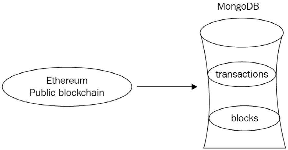
Figure 7.1: A MongoDB database interacting with the Ethereum public blockchain
Our data resides in two collections: blocks and transactions.
A sample block document has the following fields:
- The number of transactions
- The number of contracted internal transactions
- The block hash
- The parent block hash
- The mining difficulty
- The amount of gas used
- The block height
The following code shows the output data from a block:
> db.blocks.findOne()
{"_id" : ObjectId("595368fbcedea89d3f4fb0ca"),"number_transactions" : 28,
"timestamp" : NumberLong("1498324744877"),"gas_used" : 4694483,
"number_internal_transactions" : 4,
"block_hash" : "0x89d235c4e2e4e4978440f3cc1966f1ffb343b9b5cfec9e5cebc331fb810bded3",
"difficulty" : NumberLong("882071747513072"),"block_height" : 3923788
}
A sample transaction document has the following fields:
- The transaction hash
- The block height that it belongs to
- The from hash address
- The to hash address
- The transaction value
- The transaction fee
The following code shows the output data from a transaction:
> db.transactions.findOne()
{"_id" : ObjectId("59535748cedea89997e8385a"),"from" : "0x3c540be890df69eca5f0099bbedd5d667bd693f3",
"txfee" : 28594,
"timestamp" : ISODate("2017-06-06T11:23:10Z"),"value" : 0,
"to" : "0x4b9e0d224dabcc96191cace2d367a8d8b75c9c81",
"txhash" : "0xf205991d937bcb60955733e760356070319d95131a2d9643e3c48f2dfca39e77",
"block" : 3923794
}
Sample data for our database is available on GitHub at https://github.com/PacktPublishing/Mastering-MongoDB-6.x.
As curious developers who are using this novel blockchain technology, we want to analyze the Ethereum transactions. We are especially keen to do the following:
- Find the top 10 addresses that the transactions originate from.
- Find the top 10 addresses that the transactions end in.
- Find the average value per transaction, with statistics concerning the deviation.
- Find the average fee required per transaction, with statistics concerning the deviation.
- Find the time of day that the network is more active according to the number or value of transactions.
- Find the day of the week in which the network is more active according to the number or value of transactions.
We will find the top 10 addresses that the transactions originate from. To calculate this metric, first, we will count the number of occurrences with a 1 count for each one, group them by the value of the from field, and output them into a new field called count.
After this, we will sort by the value of the count field in descending (-1) order, and finally, we will limit the output to the first 10 documents that pass through the pipeline. These documents are the top 10 addresses that we are looking for.
The following is some sample Python code:
def top_ten_addresses_from(self):
pipeline = [
{"$group": {"_id": "$from", "count": {"$sum": 1}}},{"$sort": SON([("count", -1)])},{"$limit": 10},]
result = self.collection.aggregate(pipeline)
for res in result:
print(res)
The output of the preceding code is as follows:
{u'count': 38, u'_id': u'miningpoolhub_1'}{u'count': 31, u'_id': u'Ethermine'}{u'count': 30, u'_id': u'0x3c540be890df69eca5f0099bbedd5d667bd693f3'}{u'count': 27, u'_id': u'0xb42b20ddbeabdc2a288be7ff847ff94fb48d2579'}{u'count': 25, u'_id': u'ethfans.org'}{u'count': 16, u'_id': u'Bittrex'}{u'count': 8, u'_id': u'0x009735c1f7d06faaf9db5223c795e2d35080e826'}{u'count': 8, u'_id': u'Oraclize'}{u'count': 7, u'_id': u'0x1151314c646ce4e0efd76d1af4760ae66a9fe30f'}{u'count': 7, u'_id': u'0x4d3ef0e8b49999de8fa4d531f07186cc3abe3d6e'}Now, we will find the top 10 addresses where the transactions end. As we did with from, the calculation for the to addresses is exactly the same, only grouping using the to field instead of from, as shown in the following code:
def top_ten_addresses_to(self):
pipeline = [
{"$group": {"_id": "$to", "count": {"$sum": 1}}},{"$sort": SON([("count", -1)])},{"$limit": 10},]
result = self.collection.aggregate(pipeline)
for res in result:
print(res)
The output of the preceding code is as follows:
{u'count': 33, u'_id': u'0x6090a6e47849629b7245dfa1ca21d94cd15878ef'}{u'count': 30, u'_id': u'0x4b9e0d224dabcc96191cace2d367a8d8b75c9c81'}{u'count': 25, u'_id': u'0x69ea6b31ef305d6b99bb2d4c9d99456fa108b02a'}{u'count': 23, u'_id': u'0xe94b04a0fed112f3664e45adb2b8915693dd5ff3'}{u'count': 22, u'_id': u'0x8d12a197cb00d4747a1fe03395095ce2a5cc6819'}{u'count': 18, u'_id': u'0x91337a300e0361bddb2e377dd4e88ccb7796663d'}{u'count': 13, u'_id': u'0x1c3f580daeaac2f540c998c8ae3e4b18440f7c45'}{u'count': 12, u'_id': u'0xeef274b28bd40b717f5fea9b806d1203daad0807'}{u'count': 9, u'_id': u'0x96fc4553a00c117c5b0bed950dd625d1c16dc894'}{u'count': 9, u'_id': u'0xd43d09ec1bc5e57c8f3d0c64020d403b04c7f783'}Let’s find the average value per transaction, with statistics concerning the standard deviation. In this example, we are using the $avg and $stdDevPop operators of the values of the value field to calculate the statistics for this field. Using a simple $group operation, we output a single document with the ID of our choice (here, it is value) and averageValues, as shown in the following code:
def average_value_per_transaction(self):
pipeline = [
{"$group": {"_id": "value", "averageValues": {"$avg": "$value"}, "stdDevValues": {"$stdDevPop": "$value"}}},]
result = self.collection.aggregate(pipeline)
for res in result:
print(res)
The output of the preceding code is as follows:
{u'averageValues': 5.227238976440972, u'_id': u'value', u'stdDevValues': 38.90322689649576}Let’s find the average fee required per transaction, returning statistics that showcase the deviation. Average fees are similar to average values, replacing $value with $txfee, as shown in the following code:
def average_fee_per_transaction(self):
pipeline = [
{"$group": {"_id": "value", "averageFees": {"$avg": "$txfee"}, "stdDevValues": {"$stdDevPop": "$txfee"}}},]
result = self.collection.aggregate(pipeline)
for res in result:
print(res)
The output of the preceding code snippet is as follows:
{u'_id': u'value', u'averageFees': 320842.0729166667, u'stdDevValues': 1798081.7305142984}We find the time of day that the network is more active according to the number or value of transactions at specific times.
To find out the most active hour for transactions, we use the $hour operator to extract the hour field from the ISODate() field in which we stored our datetime values and called timestamp, as shown in the following code:
def active_hour_of_day_transactions(self):
pipeline = [
{"$group": {"_id": {"$hour": "$timestamp"}, "transactions": {"$sum": 1}}},{"$sort": SON([("transactions", -1)])},{"$limit": 1},]
result = self.collection.aggregate(pipeline)
for res in result:
print(res)
The output is as follows:
{u'_id': 11, u'transactions': 34}The following code will calculate the sum of transaction values for the most active hour of the day:
def active_hour_of_day_values(self):
pipeline = [
{"$group": {"_id": {"$hour": "$timestamp"}, "transaction_values": {"$sum": "$value"}}},{"$sort": SON([("transactions", -1)])},{"$limit": 1},]
result = self.collection.aggregate(pipeline)
for res in result:
print(res)
The output of the preceding code is as follows:
{u'transaction_values': 33.17773841, u'_id': 20}Let’s find the day of the week that the network is more active according to the number of transactions or the value of transactions. As we did with the hour of the day, we use the $dayOfWeek operator to extract the day of the week from the ISODate() objects, as shown in the following code. Days are numbered ranging from one for Sunday to seven for Saturday, following the US convention:
def active_day_of_week_transactions(self):
pipeline = [
{"$group": {"_id": {"$dayOfWeek": "$timestamp"}, "transactions": {"$sum": 1}}},{"$sort": SON([("transactions", -1)])},{"$limit": 1},]
result = self.collection.aggregate(pipeline)
for res in result:
print(res)
The output of the preceding code is as follows:
{u'_id': 3, u'transactions': 92}The following code will calculate the sum of transaction values for the most active day of the week:
def active_day_of_week_values(self):
pipeline = [
{"$group": {"_id": {"$dayOfWeek": "$timestamp"}, "transaction_values": {"$sum": "$value"}}}, {"$sort": SON([("transactions", -1)])}, {"$limit": 1},]
result = self.collection.aggregate(pipeline)
for res in result:
print(res)
The output of the preceding code is as follows:
{u'transaction_values': 547.62439312, u'_id': 2}The aggregations that we calculated can be described in the following diagram:
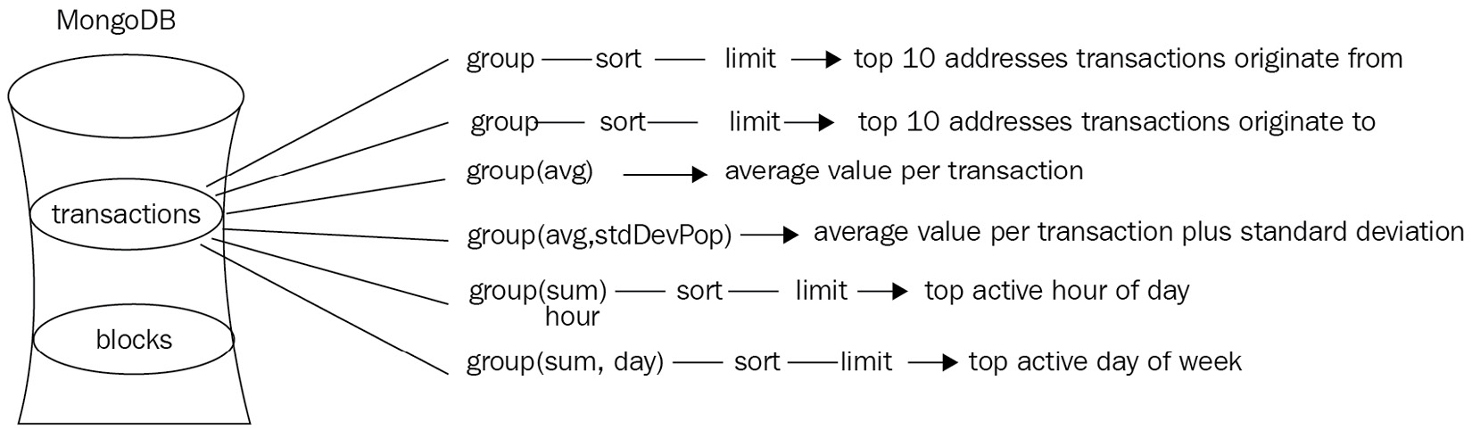
Figure 7.2: Aggregations performed in the transactions collection
In terms of blocks, we would like to know the following:
- The average number of transactions per block, for both the total number of overall transactions and the total number of contracted internal transactions.
- The average amount of gas used per block.
- The average amount of gas used per transaction to a block. Is there a window of opportunity in which to submit my smart contract in a block?
- The average level of difficulty per block and how it deviates.
- The average number of transactions per block, both in total and also in contracted internal transactions.
Averaging over the number_transactions field, we can get the number of transactions per block, as shown in the following code:
def average_number_transactions_total_block(self):
pipeline = [
{"$group": {"_id": "average_transactions_per_block", "count": {"$avg": "$number_transactions"}}},]
result = self.collection.aggregate(pipeline)
for res in result:
print(res)
The output of the preceding code is as follows:
{u'count': 39.458333333333336, u'_id': u'average_transactions_per_block'}Whereas with the following code, we can get the average number of internal transactions per block:
def average_number_transactions_internal_block(self):
pipeline = [
{"$group": {"_id": "average_transactions_internal_per_block", "count": {"$avg": "$number_internal_transactions"}}},]
result = self.collection.aggregate(pipeline)
for res in result:
print(res)
The output of the preceding code is as follows:
{u'count': 8.0, u'_id': u'average_transactions_internal_per_block'}The average amount of gas used per block can be acquired as follows:
def average_gas_block(self):
pipeline = [
{"$group": {"_id": "average_gas_used_per_block", "count": {"$avg": "$gas_used"}}},]
result = self.collection.aggregate(pipeline)
for res in result:
print(res)
The output is as follows:
{u'count': 2563647.9166666665, u'_id': u'average_gas_used_per_block'}The average difficulty per block and how it deviates can be acquired as follows:
def average_difficulty_block(self):
pipeline = [
{"$group": {"_id": "average_difficulty_per_block", "count": {"$avg": "$difficulty"}, "stddev": {"$stdDevPop": "$difficulty"}}},]
result = self.collection.aggregate(pipeline)
for res in result:
print(res)
The output is as follows:
{u'count': 881676386932100.0, u'_id': u'average_difficulty_per_block', u'stddev': 446694674991.6385}Our aggregations are described in the following diagram:
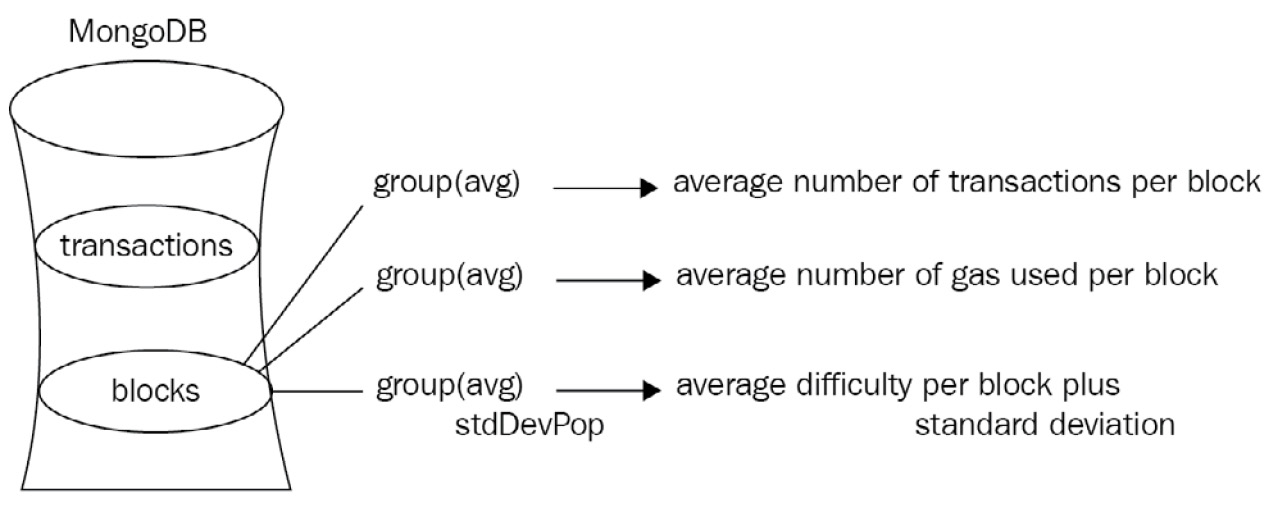
Figure 7.3: Aggregations performed in the blocks collection
Now that we have the basic statistics calculated, we want to up our game and find out more information about our transactions. Through our sophisticated machine learning algorithms, we have identified some of the transactions as either a scam or an initial coin offering (ICO), or maybe both.
In these documents, we have marked the attributes in an array called tags, as follows:
{ "_id" : ObjectId("59554977cedea8f696a416dd"),"to" : "0x4b9e0d224dabcc96191cace2d367a8d8b75c9c81",
"txhash" : "0xf205991d937bcb60955733e760356070319d95131a2d9643e3c48f2dfca39e77",
"from" : "0x3c540be890df69eca5f0099bbedd5d667bd693f3",
"block" : 3923794,
"txfee" : 28594,
"timestamp" : ISODate("2017-06-10T09:59:35Z"),"tags" : [
"scam",
"ico"
],
"value" : 0
}
Now we want to get the transactions from June 2017, remove the _id field, and produce different documents according to the tags that we have identified. So, in our example, we would output two documents in our new collection, scam_ico_documents, for separate processing.
The way to do this is via the aggregation framework, as shown in the following code:
def scam_or_ico_aggregation(self):
pipeline = [
{"$match": {"timestamp": {"$gte": datetime.datetime(2017,6,1), "$lte": datetime.datetime(2017,7,1)}}}, {"$project": {"to": 1,
"txhash": 1,
"from": 1,
"block": 1,
"txfee": 1,
"tags": 1,
"value": 1,
"report_period": "June 2017",
"_id": 0,
}
},
{"$unwind": "$tags"}, {"$out": "scam_ico_documents"}]
result = self.collection.aggregate(pipeline)
for res in result:
print(res)
Here, we have the following four distinct steps in our aggregation framework pipeline:
- Using $match, we only extract documents that have a timestamp field value of June 01, 2017.
- Using $project, we add a new report_period field with a value of June 2017 and remove the _id field by setting its value to 0. We keep the rest of the fields intact by using the value of 1, as shown in the preceding code.
- Using $unwind, we output one new document per tag in our $tags array.
- Finally, using $out, we output all of our documents to a new scam_ico_documents collection.
Since we used the $out operator, we will get no results in the command line. If we comment out {"$out": "scam_ico_documents"}, we get documents that look like the following:
{u'from': u'miningpoolhub_1', u'tags': u'scam', u'report_period': u'June 2017', u'value': 0.52415349, u'to': u'0xdaf112bcbd38d231b1be4ae92a72a41aa2bb231d', u'txhash': u'0xe11ea11df4190bf06cbdaf19ae88a707766b007b3d9f35270cde37ceccba9a5c', u'txfee': 21.0, u'block': 3923785}The final result in our database will look like this:
{ "_id" : ObjectId("5955533be9ec57bdb074074e"),"to" : "0x4b9e0d224dabcc96191cace2d367a8d8b75c9c81",
"txhash" : "0xf205991d937bcb60955733e760356070319d95131a2d9643e3c48f2dfca39e77",
"from" : "0x3c540be890df69eca5f0099bbedd5d667bd693f3",
"block" : 3923794,
"txfee" : 28594,
"tags" : "scam",
"value" : 0,
"report_period" : "June 2017"
}
Now that we have documents that are clearly separated in the scam_ico_documents collection, we can perform further analysis pretty easily. An example of this analysis would be to append more information on some of these scammers. Luckily, our data scientists have come up with some additional information that we have extracted into a new scam_details collection, which looks like this:
{ "_id" : ObjectId("5955510e14ae9238fe76d7f0"),"scam_address" : "0x3c540be890df69eca5f0099bbedd5d667bd693f3",
Email_address": [email protected]"
}
Now, we can create a new aggregation pipeline job to join scam_ico_documents with the scam_details collection and output these extended results into a new collection, called scam_ico_documents_extended, as follows:
def scam_add_information(self):
client = MongoClient()
db = client.mongo_book
scam_collection = db.scam_ico_documents
pipeline = [
{"$lookup": {"from": "scam_details", "localField": "from", "foreignField": "scam_address", "as": "scam_details"}}, {"$match": {"scam_details": { "$ne": [] }}}, {"$out": "scam_ico_documents_extended"}]
result = scam_collection.aggregate(pipeline)
for res in result:
print(res)
Here, we are using the following three-step aggregation pipeline:
- Use the $lookup command to join data from the scam_details collection and the scam_address field with data from our local collection (scam_ico_documents) based on the value from the local collection attribute, from, being equal to the value in the scam_details collection’s scam_address field. If they are equal, then the pipeline adds a new field to the document called scam_details.
- Next, we only match the documents that have a scam_details field—the ones that matched with the lookup aggregation framework step.
- Finally, we output these documents into a new collection called scam_ico_documents_extended.
These documents will now look like the following:
> db.scam_ico_documents_extended.findOne()
{ "_id" : ObjectId("5955533be9ec57bdb074074e"),"to" : "0x4b9e0d224dabcc96191cace2d367a8d8b75c9c81",
"txhash" : "0xf205991d937bcb60955733e760356070319d95131a2d9643e3c48f2dfca39e77",
"from" : "0x3c540be890df69eca5f0099bbedd5d667bd693f3",
"block" : 3923794,
"txfee" : 28594,
"tags" : "scam",
"value" : 0,
"report_period" : "June 2017",
"scam_details_data" : [
{ "_id" : ObjectId("5955510e14ae9238fe76d7f0"),"scam_address" : "0x3c540be890df69eca5f0099bbedd5d667bd693f3",
email_address": [email protected]"
}]}
Using the aggregation framework, we have identified our data and can process it rapidly and efficiently.
The previous steps can be summed up in the following diagram:
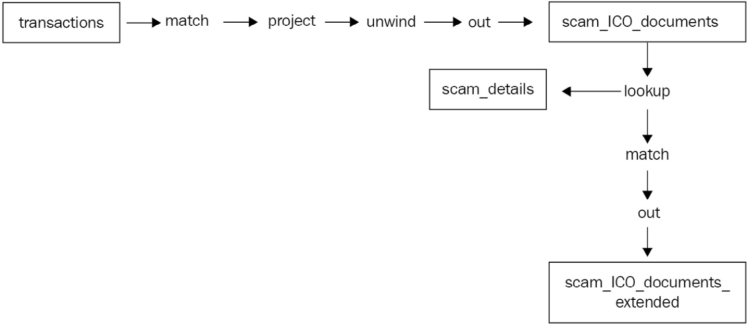
Figure 7.4: The overall data flow of our use case
Summary
In this chapter, we dived deep into the aggregation framework. We discussed why and when we should use aggregation as opposed to simply using MapReduce or querying the database. We went through a vast array of options and functionalities for aggregation.
We discussed the aggregation stages and the various operators, such as Boolean operators, comparison operators, set operators, array operators, date operators, string operators, expression arithmetic operators, aggregation accumulators, conditional expressions, and variables, along with the literal parsing data type operators.
Using the Ethereum use case, we went through aggregation with working code and learned how to approach an engineering problem to solve it.
Finally, we learned about the limitations that the aggregation framework currently has and when to avoid them.
In the next chapter, we will move on to the topic of indexing and learn how to design and implement performant indexes for our read and write workloads.