4.2.1 Parsing an XML file

We’ll start by parsing an Extensible Markup Language (XML) file to get the raw latitude and longitude pairs. This will show you how we can encapsulate some not-quite-functional features of Python to create an iterable sequence of values.

We’ll make use of the xml.etree module. After parsing, the resulting ElementTree object has an iterfind() method that will iterate through the available values.

We’ll be looking for constructs such as the following XML example:

<Placemark><Point> 
<coordinates>-76.33029518659048, 37.54901619777347,0</coordinates> 
</Point></Placemark>

The file will have a number of <Placemark> tags, each of which has a point and coordinate structure within it. The coordinate tag’s values are East-West longitude, North-South latitude, and altitude above mean sea level. This means there are two tiers of parsing: the XML tier, and then the details of each coordinate. This is typical of Keyhole Markup Language (KML) files that contain geographic information. (For more information, see https://developers.google.com/kml/documentation.)

Extracting data from an XML file can be approached at two levels of abstraction:

• At the lower level, we need to locate the various tags, attribute values, and content within the XML file.

• At a higher level, we want to make useful objects out of the text and attribute values.

The lower-level processing can be approached in the following way:

from collections.abc import Iterable 
from typing import TextIO 
import xml.etree.ElementTree as XML 
 
def row_iter_kml(file_obj: TextIO) -> Iterable[list[str]]: 
    ns_map = { 
        "ns0": "http://www.opengis.net/kml/2.2", 
        "ns1": "http://www.google.com/kml/ext/2.2" 
    } 
    path_to_points = ( 
      "./ns0:Document/ns0:Folder/ns0:Placemark/" 
      "ns0:Point/ns0:coordinates" 
    ) 
    doc = XML.parse(file_obj) 
    text_blocks = ( 
        coordinates.text 
        for coordinates in doc.iterfind(path_to_points, ns_map) 
    ) 
    return ( 
        comma_split(text) 
        for text in text_blocks 
        if text is not None 
    )

This function requires text; generally this will come from a file opened via a with statement. The result of this function is a generator that creates list objects from the latitude/longitude pairs. As a part of the XML processing, this function uses a simple static dict object, ns_map, that provides the namespace mapping information for the XML tags being parsed. This dictionary will be used by the ElementTree.iterfind() method to locate only the <coordinates> tags in the XML source document.

The essence of the parsing is a generator function that uses the sequence of tags located by doc.iterfind(). This sequence of tags is then processed by a comma_split() function to tease the text value into its comma-separated components.

The path_to_points object is a string that defines how to navigate through the XML structure. It describes the location of the <coordinates> tag within the other tags of the document. Using this path means the generator expression will avoid the values of other, irrelevant tags.

The if text is not None clause reflects the definition of the text attribute of an element tree tag. If there’s no body in the tag, the text value will be None. While it is extremely unlikely to see an empty <coordinates/> tag, the type hints require we handle this case.

The comma_split() function has a more functional syntax than the the split() method of a string. This function is defined as follows:

def comma_split(text: str) -> list[str]: 
    return text.split(",")

We’ve used a wrapper to emphasize a slightly more uniform syntax. We’ve also added explicit type hints to make it clear that a string is converted to a list of str values. Without the type hint, there are two potential definitions of split() that could be meant. It turns out, this method applies to bytes as well as str. We’ve used the str type name to narrow the domain of types.

The result of the row_iter_kml() function is an iterable sequence of rows of data. Each row will be a list composed of three strings: latitude, longitude, and altitude of a waypoint along this path. This isn’t directly useful yet. We’ll need to do some more processing to get latitude and longitude as well as converting these two strings into useful floating-point values.

This idea of an iterable sequence of tuples (or lists) allows us to process some kinds of data files in a simple and uniform way. In Chapter 3, Functions, Iterators, and Generators, we looked at how Comma-Separated Values (CSV) files are easily handled as rows of tuples. In Chapter 6, Recursions and Reductions, we’ll revisit the parsing idea to compare these various examples.

The output from the row_iter_kml() function can be collected by the list() function. The following interactive example will read the file and extract the details. The list() function will create a single list from each <coordinate> tag. The accumulated result object looks like the following example:

>>> from pprint import pprint 
>>> source_url = "file:./Winter%202012-2013.kml" 
>>> with urllib.request.urlopen(source_url) as source: 
...     v1 = list(row_iter_kml(source)) 
>>> pprint(v1) 
[[’-76.33029518659048’, ’37.54901619777347’, ’0’], 
 [’-76.27383399999999’, ’37.840832’, ’0’], 
 [’-76.459503’, ’38.331501’, ’0’], 
 ... 
 [’-76.47350299999999’, ’38.976334’, ’0’]]

These are all string values. To be more useful, it’s important to apply some additional functions to the output of this function that will create a usable subset of the data.

4.2.2 Parsing a file at a higher level

After parsing the low-level syntax to transform XML to Python, we can restructure the raw data into something usable in our Python program. This kind of structuring applies to XML, JavaScript Object Notation (JSON), CSV, YAML, TOML, and any of the wide variety of physical formats in which data is serialized.

We’ll aim to write a small suite of generator functions that transforms the parsed data into a form our application can use. The generator functions include some simple transformations on the text that are found by the row_iter_kml() function, which are as follows:

• Discarding altitude, which can also be stated as keeping only latitude and longitude

• Changing the order from (longitude, latitude) to (latitude, longitude)

We can make these two transformations have more syntactic uniformity by defining a utility function, as follows:

def pick_lat_lon( 
        lon: str, lat: str, alt: str 
) -> tuple[str, str]: 
    return lat, lon

We’ve created a function to take three argument values and create a tuple from two of them. The type hints are more complex than the function itself. The conversion of source data to usable data often involves selecting a subset of fields, as well as conversion from strings to numbers. We’ve separated the two problems because these aspects often evolve separately.

We can use this function as follows:

from collections.abc import Iterable 
from typing import TypeAlias 
 
Rows: TypeAlias = Iterable[list[str]] 
LL_Text: TypeAlias = tuple[str, str] 
 
def lat_lon_kml(row_iter: Rows) -> Iterable[LL_Text]: 
    return (pick_lat_lon(*row) for row in row_iter)

This function will apply the pick_lat_lon() function to each row from a source iterator. We’ve used *row to assign each element of the row’s three-tuple to separate parameters of the pick_lat_lon() function. The function can then extract and reorder the two relevant values from each three-tuple.

To simplify the function definition, we’ve defined two type aliases: Rows and LL_Text. These type aliases can simplify a function definition. They can also be reused to ensure that several related functions are all working with the same types of objects. This kind of functional design allows us to freely replace any function with its equivalent, which makes refactoring less risky.

These functions can be combined to parse the file and build a structure we can use. Here’s an example of some code that could be used for this purpose:

>>> import urllib 
>>> source_url = "file:./Winter%202012-2013.kml" 
>>> with urllib.request.urlopen(source_url) as source: 
...     v1 = tuple(lat_lon_kml(row_iter_kml(source))) 
>>> v1[0] 
(’37.54901619777347’, ’-76.33029518659048’) 
>>> v1[-1] 
(’38.976334’, ’-76.47350299999999’)

This script uses the request.urlopen() function to open a source. In this case, it’s a local file. However, we can also open a KML file on a remote server. Our objective in using this kind of file opening is to ensure that our processing is uniform no matter what the source of the data is.

The script is built around the two functions that do low-level parsing of the KML source. The row_iter_kml(source) expression produces a sequence of text columns. The lat_lon_kml() function will extract and reorder the latitude and longitude values. This creates an intermediate result that sets the stage for further processing. The subsequent processing can be designed to be independent of the original format.

The final function provides the latitude and longitude values from a complex XML file using an almost purely functional approach. As the result is iterable, we can continue to use functional programming techniques to process each point that we retrieve from the file.

This design explicitly separates low-level XML parsing from higher-level reorganization of the data. The XML parsing produced a generic tuple of string structure. This is compatible with parsers for other file formats. As one example, the result value is compatible with the output from the CSV parser. When working with SQL databases, it can help to use a similar iterable of tuple structures. This permits a design for higher-level processing that can work with data from a variety of sources.

We’ll show you a series of transformations to re-arrange this data from a collection of strings to a collection of waypoints along a route. This will involve a number of transformations. We’ll need to restructure the data as well as convert from strings to floating-point values. We’ll also look at a few ways to simplify and clarify the subsequent processing steps. We’ll use this dataset in later chapters because it’s quite complex.

4.2.3 Pairing up items from a sequence

A common restructuring requirement is to make start-stop pairs out of points in a sequence. Given a sequence, S = {s₀,s₁,s₂,...,s_n}, we would also want to create a paired sequence, S = {(s₀,s₁),(s₁,s₂),(s₂,s₃),...,(s_n−1,s_n)}. The first and second items form a pair. The second and third items form the next pair. Note that the pairs overlap; each point (other than the first or last) will be the end of one pair and the start of the next pair.

These overlapping pairs are used to compute distances from point to point using a trivial application of a haversine function. This technique is also used to convert a path of points into a series of line segments in a graphics application.

Why pair up items? Why not insert a few additional lines of code into a function such as this:

begin = next(iterable) 
for end in iterable: 
    compute_something(begin, end) 
    begin = end

This code snippet will process each leg of the data as a begin, end pair. However, the processing function and the for statement to restructure the data are tightly bound, making reuse more complex than necessary. The algorithm for pairing is hard to test in isolation when it is one part of a more complex compute_something() function.

Creating a combined function also limits our ability to reconfigure the application. There’s no easy way to inject an alternative implementation of the compute_something() function. Additionally, we’ve got a piece of an explicit state, the begin variable, which makes life potentially complex. If we try to add features to the body of the for statement, we can easily fail to set the begin variable correctly when an item in the iterable source is filtered out from processing.

We achieve better reuse by separating this pairing function from other processing. Simplification, in the long run, is one of our goals. If we build up a library of helpful primitives such as this pairing function, we can tackle larger problems more quickly and confidently.

There are many ways to pair up the points along the route to create start and stop information for each leg. We’ll look at a few here and then revisit this in Chapter 5, Higher-Order Functions, and again in Chapter 8, The Itertools Module. Creating pairs can be done in a purely functional way using a recursion:

While the mathematical formalism seems simple, it doesn’t account for the way item l₁ is both part of the first pair and also the head of the remaining items in l_[1:].

The functional ideal is to avoid assigning this value to a variable. Variables—and the resulting stateful code—can turn into a problem when we try to make a ”small” change and misuse the variable’s value.

An alternative is to somehow ”peek” at the upcoming item in the iterable source of data. This doesn’t work out well in Python. Once we’ve used next() to examine the value, it can’t be put back into the iterable. This makes a recursive, functional version of creating overlapping pairs a bit too complex to be of any real value.

Our strategy for performing tail-call optimization is to replace the recursion in the mathematical formalism with a for statement. In some cases, we can further optimize this into a generator expression. Because this works with an explicit variable to track the state of the computation, it’s a better fit for Python, while being less purely functional.

The following code is an optimized version of a function to pair up the points along a route:

from collections.abc import Iterator, Iterable 
from typing import Any, TypeVar 
 
LL_Type = TypeVar(’LL_Type’) 
 
def legs(lat_lon_iter: Iterator[LL_Type]) -> Iterator[tuple[LL_Type, LL_Type]]: 
    begin = next(lat_lon_iter) 
    for end in lat_lon_iter: 
        yield begin, end 
        begin = end

The version is simpler, quite fast, and free from the stack limits of a recursive definition. It’s independent of any particular type of sequence, as it will pair up anything emitted by a sequence generator. As there’s no processing function inside the loop, we can reuse the legs() function as needed. We could also redesign this function slightly to accept a processing function as a parameter value, and apply the given function to each (begin, end) pair that’s created.

The type variable, LL_Type, is used to clarify precisely how the legs() function restructures the data. The hint says that the input type is preserved on output. The input type is an Iterator of some arbitrary type, LL_Type; the output will include tuples of the same type, LL_Type. No other conversion is implied by the function.

The begin and end variables maintain the state of the computation. The use of stateful variables doesn’t fit the ideal of using immutable objects for functional programming. The optimization, however, is important in Python. It’s also invisible to users of the function, making it a Pythonic-functional hybrid.

Note that this function requires an iterable source of individual values. This can be an iterable collection or a generator.

We can think of this function as one that yields the following kind of sequence of pairs:

[items[0:2], items[1:3], items[2:4], ..., items[-2:]]

Another view of this function using the built-in zip() function is as follows:

list(zip(items, items[1:]))

While informative, this zip()-based example only works for sequence objects. The pairs() function shown earlier will work for any iterable, including sequence objects. The legs() function only works for an Iterator object as the source of data. The good news is we can make an iterator object from an iterable collection with the built-in iter() function.

4.2.4 Using the iter() function explicitly

From a purely functional viewpoint, all of our iterables can be processed with recursive functions, where the state is managed by the recursive call stack. Pragmatically, processing iterables in Python will often involve evaluation of for statements. There are two common situations: collection objects and iterables. When working with a collection object, an Iterator object is created by the for statement. When working with a generator function, the generator function is an iterator and maintains its own internal state. Often, these are equivalent, from a Python programming perspective. In rare cases—generally those situations where we have to use the next() function explicitly—the two won’t be precisely equivalent.

The legs() function shown previously has an explicit next() evaluation to get the first value from the iterable. This works wonderfully well with generator functions, expressions, and other iterables. It doesn’t work with sequence objects such as tuples or lists.

The following code contains three examples to clarify the use of the next() and iter() functions:

# Iterator as input: 
>>> list(legs(x for x in range(3))) 
[(0, 1), (1, 2)] 
 
# List object as input: 
>>> list(legs([0, 1, 2])) 
Traceback (most recent call last): 
... 
TypeError: ’list’ object is not an iterator 
 
# Explicit iterator created from list object: 
>>> list(legs(iter([0,1,2]))) 
[(0, 1), (1, 2)]

In the first case, we applied the legs() function to an iterable. In this case, the iterable was a generator expression. This is the expected behavior based on our previous examples in this chapter. The items are properly paired up to create two legs from three waypoints.

In the second case, we tried to apply the legs() function to a sequence. This resulted in an error. While a list object and an iterable are equivalent when used in a for statement, they aren’t equivalent everywhere. A sequence isn’t an iterator; a sequence doesn’t implement the __next__() special method allowing it to be used by the next() function. The for statement handles this gracefully, however, by creating an iterator from a sequence automatically.

To make the second case work, we need to explicitly create an iterator from a list object. This permits the legs() function to get the first item from the iterator over the list items. The iter() function will create an iterator from a list.

4.2.5 Extending an iteration

We have two kinds of extensions we could factor into a for statement that processes iterable data. We’ll look first at a filter extension. In this case, we may be rejecting values from further consideration. They may be data outliers, or perhaps source data that’s improperly formatted. Then, we’ll look at mapping source data by performing a simple transformation to create new objects from the original objects. In our case, we’ll be transforming strings to floating-point numbers. The idea of extending a simple for statement with a mapping, however, applies to many situations. We’ll look at refactoring the above legs() function. What if we need to adjust the sequence of points to discard a value? This will introduce a filter extension that rejects some data values.

The iterative process we’re designing returns pairs without performing any additional application-related processing—the complexity is minimal. Simplicity means we’re somewhat less likely to confuse the processing state.

Adding a filter extension to this design could look something like the following code snippet:

from collections.abc import Iterator, Iterable, Callable 
from typing import TypeAlias 
 
Waypoint: TypeAlias = tuple[float, float] 
Pairs_Iter: TypeAlias = Iterator[Waypoint] 
Leg: TypeAlias = tuple[Waypoint, Waypoint] 
Leg_Iter: TypeAlias = Iterable[Leg] 
 
def legs_filter( 
        lat_lon_iter: Pairs_Iter, 
        rejection_rule: Callable[[Waypoint, Waypoint], bool]) -> Leg_Iter: 
    begin = next(lat_lon_iter) 
    for end in lat_lon_iter: 
        if rejection_rule(begin, end): 
            pass 
        else: 
            yield begin, end 
        begin = end

We have plugged in a processing rule to reject certain values. As the for statement remains succinct and expressive, we are confident that the processing will be done properly. We have, on the other hand, cluttered up a relatively simple function with two separate collections of features. This kind of clutter is not an ideal approach to functional design.

We haven’t really provided much information about the rejection_rule() function. This needs to be a kind of condition that applies to a Leg tuple to reject the point from further consideration. For example, it may reject begin == end to avoid zero-length legs. A handy default value for rejection_rule is lambda s, e: False. This will preserve all of the legs.

The next refactoring will introduce additional mapping to an iteration. Adding mappings is common when a design is evolving. In our case, we have a sequence of string values. We need to convert these to float values for later use.

The following is one way to handle this data mapping, through a generator expression that wraps a generator function:

>>> import urllib 
>>> source_url = "file:./Winter%202012-2013.kml" 
>>> with urllib.request.urlopen(source_url) as source: 
...     trip = list( 
...         legs( 
...            (float(lat), float(lon)) 
...            for lat, lon in lat_lon_kml(row_iter_kml(source)) 
...         ) 
...     )

We’ve applied the legs() function to a generator expression that creates float values from the output of the lat_lon_kml() function. We can read this in an inside-out order as well. The lat_lon_kml() function’s output is transformed into a pair of float values, which is then transformed into a sequence of legs.

This is starting to get complex. We’ve got a large number of nested functions here. We’re applying float(), legs(), and list() to a data generator. One common way of refactoring complex expressions is to separate the generator expression from any materialized collection. We can do the following to simplify the expression:

>>> import urllib 
>>> source_url = "file:./Winter%202012-2013.kml" 
>>> with urllib.request.urlopen(source_url) as source: 
...     ll_iter = ( 
...         (float(lat), float(lon)) 
...         for lat, lon in lat_lon_kml(row_iter_kml(source)) 
...     ) 
...     trip = list( 
...         legs(ll_iter) 
...     )

We’ve assigned the generator function to a variable named ll_iter. This variable isn’t a collection object; it’s a generator of item two-tuples. We’re not using a list comprehension to create an object. We’ve merely assigned the generator expression to a variable name. We’ve then used the ll_iter variable in a subsequent expression.

The evaluation of the list() function actually leads to a proper object being built so that we can print the output. The ll_iter variable’s items are created only as needed.

There is yet another refactoring we might like to do. In general, the source of the data is something we often want to change. In our example, the lat_lon_kml() function is tightly bound in the rest of the expression. This makes reuse difficult when we have a different data source.

In the case where the float() operation is something we’d like to parameterize so that we can reuse it, we can define a function around the generator expression. We’ll extract some of the processing into a separate function merely to group the operations. In our case, the string-pair to float-pair is unique to particular source data. We can rewrite a complex float-from-string expression into a simpler function, such as:

from collections.abc import Iterator, Iterable 
from typing import TypeAlias 
 
Text_Iter: TypeAlias = Iterable[tuple[str, str]] 
LL_Iter: TypeAlias = Iterable[tuple[float, float]] 
 
def floats_from_pair(lat_lon_iter: Text_Iter) -> LL_Iter: 
    return ( 
        (float(lat), float(lon)) 
        for lat, lon in lat_lon_iter 
    )

The floats_from_pair() function applies the float() function to the first and second values of each item in the iterable, yielding a two-tuple of floats created from an input value. We’ve relied on Python’s for statement to decompose the two-tuple.

The type hints detail the transformation from an iterable sequence of tuple[str, str] items to tuple[float, float] items. The LL_Iter type alias can then be used elsewhere in a complex set of function definitions to show how the float pairs are processed.

We can use this function in the following context:

>>> import urllib 
>>> source_url = "file:./Winter%202012-2013.kml" 
>>> with urllib.request.urlopen(source_url) as source: 
...     trip = list( 
...         legs( 
...             floats_from_pair( 
...                 lat_lon_kml( 
...                     row_iter_kml(source)))) 
...     )

We’re going to create legs that are built from float values that come from a KML file. It’s fairly easy to visualize the processing, as each stage in the process is a prefix function. Each function’s input is the output from the next function in the nested processing steps. This seems like a natural way to express a pipeline of processing.

When parsing, we often have sequences of string values. For numeric applications, we’ll need to convert strings to float, int, or Decimal values. This often involves inserting a function such as the floats_from_pair() function into a sequence of expressions that clean up the source data.

Our previous output was all strings; it looked like the following code snippet:

((’37.54901619777347’, ’-76.33029518659048’), 
 (’37.840832’, ’-76.27383399999999’), 
 ... 
 (’38.976334’, ’-76.47350299999999’))

We’ll want data like the following code snippet, where we have floats:

(((37.54901619777347, -76.33029518659048), 
(37.840832, -76.273834)), ((37.840832, -76.273834), 
... 
((38.330166, -76.458504), (38.976334, -76.473503)))

After building this processing pipeline, there are some simplifications available. We’ll look at some refactoring in Chapter 5, Higher-Order Functions. We will revisit this in Chapter 6, Recursions and Reductions, to see how to apply these simplifications to the file parsing problem.

4.2.6 Applying generator expressions to scalar functions

We’ll look at a more complex kind of generator expression to map data values from one kind of data to another. In this case, we’ll apply a fairly complex function to individual data values created by a generator.

We’ll call these non-generator functions scalar, as they work with simple atomic values. To work with collections of data, a scalar function will be embedded in a generator expression.

To continue the example started earlier, we’ll provide a haversine function to compute the distance between latitude and longitude values. Technically, these are angles, and some spherical trigonometry is required to convert angles to distances on the surface of the sphere. We can use a generator expression to apply a scalar haversine() function to a sequence of pairs from our KML file.

The important part of the haversine() function is to compute a distance between two points following the proper spherical geometry of the earth. It can involve some tricky-looking math, but we’ve provided the whole definition here. We also mentioned this function at the beginning of the Working with iterables section.

The haversine() function is implemented by the following code:

from math import radians, sin, cos, sqrt, asin 
from typing import TypeAlias 
 
MI = 3959 
NM = 3440 
KM = 6371 
 
Point: TypeAlias = tuple[float, float] 
 
def haversine(p1: Point, p2: Point, R: float=NM) -> float: 
    lat_1, lon_1 = p1 
    lat_2, lon_2 = p2 
    Δ_lat = radians(lat_2 - lat_1) 
    Δ_lon = radians(lon_2 - lon_1) 
    lat_1 = radians(lat_1) 
    lat_2 = radians(lat_2) 
 
    a = sqrt( 
        sin(Δ_lat / 2) ** 2 + 
        cos(lat_1) * cos(lat_2) * sin(Δ_lon / 2) ** 2 
    ) 
    c = 2 * asin(a) 
    return R * c

The start and end points, p1 and p2, have type hints to show their structure. The return value is also provided with a hint. The explicit use of a type alias for Point makes it possible for the mypy tool to confirm that this function is used properly.

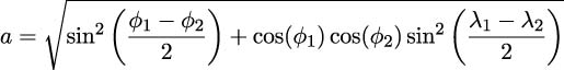
For short distances covered by coastal sailors, the equirectangular distance computation is more useful:

Where R is the earth’s mean radius, R = nautical miles. The ϕ values are N-S latitude, and the λ values are E-W longitude. This means (ϕ₀,λ₀) and (ϕ₁,λ₁) are the two points we’re navigating between.

See https://edwilliams.org/avform147.htm for more information.

The following code is how we could use our collection of functions to examine some KML data and produce a sequence of distances:

>>> import urllib 
>>> source_url = "file:./Winter%202012-2013.kml" 
>>> with urllib.request.urlopen(source_url) as source: 
...     trip = ( 
...         (start, end, round(haversine(start, end), 4)) 
...         for start,end in 
...             legs( 
...                 floats_from_pair( 
...                     lat_lon_kml(row_iter_kml(source)) 
...                 ) 
...             ) 
...     ) 
...     for start, end, dist in trip: 
...         print(f"({start} to {end} is {dist:.1f}")

The essence of the processing is the generator expression assigned to the trip variable. We’ve assembled three-tuples with a start, end, and the distance from start to end. The start and end pairs come from the legs() function. The legs() function works with floating-point data built from the latitude-longitude pairs extracted from a KML file.

The output looks like the following command snippet:

((37.54901619777347, -76.33029518659048) to (37.840832, -76.273834) is 17.7 
((37.840832, -76.273834) to (38.331501, -76.459503) is 30.7 
((38.331501, -76.459503) to (38.845501, -76.537331) is 31.1 
((38.845501, -76.537331) to (38.992832, -76.451332) is 9.7 
...

Each individual processing step has been defined succinctly. The overview, similarly, can be expressed succinctly as a composition of functions and generator expressions.

Clearly, there are several further processing steps we may like to apply to this data. The first, of course, is to use the format() method of a string to produce better-looking output.

More importantly, there are a number of aggregate values we’d like to extract from this data. We’ll call these values reductions of the available data. We’d like to reduce the data to get the maximum and minimum latitude, for example, to show the extreme north and south ends of this route. We’d like to reduce the data to get the maximum distance in one leg as well as the total distance for all legs.

The problem we’ll have using Python is that the output generator in the trip variable can be used only once. We can’t easily perform several reductions of this detailed data. While we can use itertools.tee() to work with the iterable several times, it takes a fair amount of memory. It can be wasteful, also, to read and parse the KML file for each reduction. We can make our processing more efficient by materializing intermediate results as a list object.

In the next section, we look at two specific kinds of reductions that compute a single boolean result from a collection of booleans.

4.4.1 Using sums and counts for statistics

In this section, we’ll implement a number of functions useful for statistics. The point is show how functional programming can be applied to the kinds of processing that are common in statistical functions.

Several common functions are described as ”measure of central tendency”. Functions like the arithmetic mean or the standard deviation provide a summary of a collection of values. A transformation called ”normalization” shifts and scales values around a population mean and standard deviation. We’ll also look at how to compute a coefficient of correlation to show to what extent two sets of data are related to each other.

The arithmetic mean seems to have an appealingly trivial definition based on sum() and len(). It looks like the following might work:

def mean(items): 
    return sum(items) / len(items)

This simple-looking function doesn’t work for Iterable objects. This definition only works for collections that support the len() function. This is easy to discover when trying to write proper type annotations. The definition of mean(items: Iterable[float]) -> float won’t work because more general Iterable[float] types don’t support len().

Indeed, we have a hard time performing a computation like standard deviation based on iterables. In Python, we must either materialize a sequence object or resort to somewhat more complex processing that computes multiple sums on a single pass through the data. To use simpler functions means using a list() to create a concrete sequence that can be processed multiple times.

To pass muster with mypy, the definition needs to look like this:

from collections.abc import Sequence 
 
def mean(items: Sequence[float]) -> float: 
    return sum(items)/len(items)

This includes the appropriate type hints to ensure that sum() and len() will both work for the expected types of data. The mypy tool is aware of the arithmetic type matching rules: any value that could be treated as a float would be considered valid. This means that mean([1, 2, 3]) will be accepted by the mypy tool in spite of the values being all integers.

We have some alternative and elegant expressions for mean and standard deviation in the following definitions:

import math 
from collections.abc import Sequence 
 
def stdev(data: Sequence[float]) -> float: 
 
    s0 = len(data)  # sum(1 for x in data) 
    s1 = sum(data)  # sum(x for x in data) 
    s2 = sum(x**2 for x in data) 
 
    mean = s1 / s0 
    stdev = math.sqrt(s2 / s0 - mean ** 2) 
    return stdev

These three sums, s0, s1, and s2, have a tidy, parallel structure. We can easily compute the mean from two of the sums. The standard deviation is a bit more complex, but it’s based on the three available sums.

This kind of pleasant symmetry also works for more complex statistical functions, such as correlation and even least-squares linear regression.

The moment of correlation between two sets of samples can be computed from their standardized value. The following is a function to compute the standardized value:

def z(x: float, m_x: float, s_x: float) -> float: 
    return (x - m_x) / s_x

The calculation subtracts the mean, μ_x, from each sample, x, and divides it by the standard deviation, σ_x. This gives us a value measured in units of sigma, σ. For normally-distributed data, a value ±1σ is expected about two-thirds of the time. More extreme values should be less common. A value outside ±3σ should happen less than one percent of the time.

We can use this scalar function as follows:

>>> d = [2, 4, 4, 4, 5, 5, 7, 9] 
>>> list(z(x, mean(d), stdev(d)) for x in d) 
[-1.5, -0.5, -0.5, -0.5, 0.0, 0.0, 1.0, 2.0]

We’ve built a list that consists of normalized scores based on some raw data in the variable, d. We used a generator expression to apply the scalar function, z(), to the sequence object.

The mean() and stdev() functions are based on the examples shown previously:

from math import sqrt 
from collections.abc import Sequence 
 
def mean(samples: Sequence[float]) -> float: 
    return s1(samples)/s0(samples) 
 
def stdev(samples: Sequence[float]) -> float: 
    N = s0(samples) 
    return sqrt((s2(samples) / N) - (s1(samples) / N) ** 2)

The three sum functions, similarly, can be defined as shown in the following code:

def s0(samples: Sequence[float]) -> float: 
    return sum(1 for x in samples)  # or len(data) 
 
def s1(samples: Sequence[float]) -> float: 
    return sum(x for x in samples)  # or sum(data) 
 
def s2(samples: Sequence[float]) -> float: 
    return sum(x*x for x in samples)

While this is very expressive and succinct, it’s a little frustrating because we can’t use an iterable here. When evaluating the mean() function, for example, both a sum of the iterable and a count of the iterable are required. For the standard deviation, two sums and a count of the iterable are all required. For this kind of statistical processing, we must materialize a sequence object (in other words, create a list) so that we can examine the data multiple times.

The following code shows how we can compute the correlation between two sets of samples:

def corr(samples1: Sequence[float], samples2: Sequence[float]) -> float: 
    m_1, s_1 = mean(samples1), stdev(samples1) 
    m_2, s_2 = mean(samples2), stdev(samples2) 
    z_1 = (z( x, m_1, s_1 ) for x in samples1) 
    z_2 = (z( x, m_2, s_2 ) for x in samples2) 
    r = ( 
        sum(zx1 * zx2 for zx1, zx2 in zip(z_1, z_2)) 
        / len(samples1) 
    ) 
    return r

This correlation function, corr(), gathers basic statistical summaries of the two sets of samples: the mean and standard deviation. Given these summaries, we define two generator functions that will create normalized values for each set of samples. We can then use the zip() function (see the next example) to pair up items from the two sequences of normalized values and compute the product of those two normalized values. The average of the product of the normalized scores is the correlation.

The following code is an example of gathering the correlation between two sets of samples:

>>> xi = [1.47, 1.50, 1.52, 1.55, 1.57, 1.60, 1.63, 1.65, 
... 1.68, 1.70, 1.73, 1.75, 1.78, 1.80, 1.83,] 
 
>>> yi = [52.21,53.12,54.48,55.84,57.20,58.57,59.93,61.29, 
... 63.11, 64.47, 66.28, 68.10, 69.92, 72.19, 74.46,] 
 
>>> round(corr(xi, yi), 5) 
0.99458

We’ve shown two sequences of data points, xi and yi. The correlation is over 0.99, which shows a very strong relationship between the two sequences.

This shows one of the strengths of functional programming. We’ve created a handy statistical module using a half-dozen functions with definitions that are single expressions. Interestingly, the the corr() function can’t easily be reduced to a single expression. (It can be reduced to a single very long expression, but it would be terribly hard to read.) Each internal variable in this function’s implementation is used only once. This shows us that the corr() function has a functional design, even though it’s written out in six separate lines of Python.

4.5.1 Unzipping a zipped sequence

We can use zip() to create a sequence of tuples. We also need to look at several ways to unzip a collection of tuples into separate collections.

The first way to unzip tuples is something we’ve seen many times: we can use a generator function to unzip a sequence of tuples. For example, assume that the following pairs are a sequence object with two-tuples:

>>> p0 = list(x[0] for x in pairs) 
>>> p0[:3] 
[1.47, 1.5, 1.52] 
>>> p1 = list(x[1] for x in pairs) 
>>> p1[:3] 
[52.21, 53.12, 54.48]

This snippet created two sequences. The p0 sequence has the first element of each two-tuple; the p1 sequence has the second element of each two-tuple.

Under some circumstances, we can use the multiple assignment of a for statement to decompose the tuples. The following is an example that computes the sum of the products:

>>> round(sum(p0*p1 for p0, p1 in pairs), 3) 
1548.245

We used the for statement to decompose each two-tuple into p0 and p1.

4.5.2 Flattening sequences

Sometimes, we’ll have zipped data that needs to be flattened. That is, we need to turn a sequence of sub-sequences into a single list. For example, our input could be a file that has rows of columnar data. It looks like this:

2 3 5 7 11 13 17 19 23 29 
31 37 41 43 47 53 59 61 67 71 
...

We can use (line.split() for line in file) to create a sequence from the lines in the source file. Each item within that sequence will be a nested 10-item tuple from the values on a single line.

This creates data in blocks of 10 values. It looks as follows:

>>> blocked = list(line.split() for line in file) 
>>> from pprint import pprint 
>>> pprint(blocked) 
[[’2’, ’3’, ’5’, ’7’, ’11’, ’13’, ’17’, ’19’, ’23’, ’29’], 
 [’31’, ’37’, ’41’, ’43’, ’47’, ’53’, ’59’, ’61’, ’67’, ’71’], 
 ... 
 [’179’, ’181’, ’191’, ’193’, ’197’, ’199’, ’211’, ’223’, ’227’, ’229’]]

This is a start, but it isn’t complete. We want to get the numbers into a single, flat sequence. Each item in the input is a 10-tuple; we’d rather not deal with decomposing this one item at a time.

We can use a two-level generator expression, as shown in the following code snippet, for this kind of flattening:

>>> len(blocked) 
5 
>>> (x for line in blocked for x in line) 
<generator object <genexpr> at ...> 
>>> flat = list(x for line in blocked for x in line) 
>>> len(flat) 
50 
>>> flat[:10] 
[’2’, ’3’, ’5’, ’7’, ’11’, ’13’, ’17’, ’19’, ’23’, ’29’]

The first for clause assigns each item—a list of 10 values—from the blocked list to the line variable. The second for clause assigns each individual string from the line variable to the x variable. The final generator is this sequence of values assigned to the x variable.

We can understand this via a rewrite as follows:

from collections.abc import Iterable 
from typing import Any 
 
def flatten(data: Iterable[Iterable[Any]]) -> Iterable[Any]: 
    for line in data: 
        for x in line: 
            yield x

This transformation shows us how the generator expression works. The first for clause (for line in data) steps through each 10-tuple in the data. The second for clause (for x in line) steps through each item in the first for clause.

This expression flattens a sequence-of-sequence structure into a single sequence. More generally, it flattens any iterable that contains iterables into a single, flat iterable. It will work for list-of-list as well as list-of-set or any other combination of nested iterables.

4.5.3 Structuring flat sequences

Sometimes, we’ll have raw data that is a flat list of values that we’d like to bunch up into subgroups. In the Pairing up items from a sequence section earlier in this chapter, we looked at overlapping pairs. In this section, we’re looking at non-overlapping pairs.

One approach is to use the itertools module’s groupby() function to implement this. This will have to wait until Chapter 8, The Itertools Module.

Let’s say we have a flat list, as follows:

>>> flat = [’2’, ’3’, ’5’, ’7’, ’11’, ’13’, ’17’, ’19’, ’23’, ’29’, 
... ’31’, ’37’, ’41’, ’43’, ’47’, ’53’, ’59’, ’61’, ’67’, ’71’, 
... ]

We can write nested generator functions to build a sequence-of-sequence structure from flat data. To do this, we’ll need a single iterator that we can use multiple times. The expression looks like the following code snippet:

>>> flat_iter = iter(flat) 
>>> (tuple(next(flat_iter) for i in range(5)) 
...     for row in range(len(flat) // 5) 
... ) 
<generator object <genexpr> at ...> 
 
>>> grouped = list(_) 
>>> from pprint import pprint 
>>> pprint(grouped) 
[(’2’, ’3’, ’5’, ’7’, ’11’), 
 (’13’, ’17’, ’19’, ’23’, ’29’), 
 (’31’, ’37’, ’41’, ’43’, ’47’), 
 (’53’, ’59’, ’61’, ’67’, ’71’)]

First, we create an iterator that exists outside either of the two loops that we’ll use to create our sequence-of-sequences. The generator expression uses tuple(next(flat_iter)for i in range(5)) to create five-item tuples from the iterable values in the flat_iter variable. This expression is nested inside another generator that repeats the inner loop the proper number of times to create the required sequence of values.

This works only when the flat list is divided evenly. If the last row has partial elements, we’ll need to process them separately.

We can use this kind of function to group data into same-sized tuples, with an odd-sized tuple at the end, using the following definitions:

from collections.abc import Sequence 
from typing import TypeVar 
 
ItemType = TypeVar("ItemType") 
# Flat = Sequence[ItemType] 
# Grouped = list[tuple[ItemType, ...]] 
 
def group_by_seq(n: int, sequence: Sequence[ItemType]) -> list[tuple[ItemType,...]]: 
    flat_iter = iter(sequence) 
    full_sized_items = list( 
        tuple(next(flat_iter) for i in range(n)) 
        for row in range(len(sequence) // n) 
    ) 
    trailer = tuple(flat_iter) 
    if trailer: 
        return full_sized_items +  [trailer] 
    else: 
        return full_sized_items

Within the group_by_seq() function, an initial list is built and assigned to the variable full_sized_items. Each tuple in this list is of size n. If there are leftovers, the trailing items are used to build a tuple with a non-zero length that we can append to the list of full-sized items. If the trailer tuple is of the length zero, it can be safely ignored.

The type hints include a generic definition of ItemType as a type variable. The intent of a type variable is to show that whatever type is an input to this function will be returned from the function. A sequence of strings or a sequence of floats would both work properly.

The input is summarized as a Sequence of items. The output is a List of tuples of items. The items are all of a common type, described with the ItemType type variable.

This isn’t as delightfully simple and functional-looking as other algorithms we’ve looked at. We can rework this into a simpler generator function that yields an iterable instead of a list.

The following code uses a while statement as part of tail recursion optimization:

from collections.abc import Iterator 
from typing import TypeVar 
 
ItemT = TypeVar("ItemT") 
 
def group_by_iter(n: int, iterable: Iterator[ItemT]) -> Iterator[tuple[ItemT, ...]]: 
    def group(n: int, iterable: Iterator[ItemT]) -> Iterator[ItemT]: 
        for i in range(n): 
            try: 
                yield next(iterable) 
            except StopIteration: 
                return 
 
    while row := tuple(group(n, iterable)): 
        yield row

We’ve created a row of the required length from the input iterable. At the end of the input iterable, the value of tuple(next(iterable) for i in range(n)) will be a zero-length tuple. This can be the base case of a recursive definition. This was manually optimized into the terminating condition of the while statement.

The walrus operator, :=, is used to assign the result of the expression tuple(group(n, iterable)) to a variable, row. If this is a non-empty tuple, it will be the output from the yield statement. If this is an empty tuple, the loop will terminate.

The type hints have been modified to reflect the way this works with an iterator. These iteration processing techniques are not limited to sequences. Because the internal group() function uses next() explicitly, it has to be used like this: group_by_iter(7, iter(flat)). The iter() function must be used to create an iterator from a collection.

We can, as an alternative, use the iter() function inside the group() function. When presented with a collection, this will create a fresh, new iterator. When presented with an iterator, it will do nothing. This makes the function easier to use.

4.5.4 Structuring flat sequences – an alternative approach

Let’s say we have a simple, flat list and we want to create non-overlapping pairs from this list. The following is the data we have:

>>> flat = [’2’, ’3’, ’5’, ’7’, ’11’, ’13’, ’17’, ’19’, ’23’, ’29’, 
...     ’31’, ’37’, ’41’, ’43’, ’47’, ’53’, ’59’, ’61’, ’67’, ’71’, 
... ]

We can create pairs using list slices, as follows:

>>> pairs = list(zip(flat[0::2], flat[1::2])) 
>>> pairs[:3] 
[(’2’, ’3’), (’5’, ’7’), (’11’, ’13’)] 
>>> pairs[-3:] 
[(’47’, ’53’), (’59’, ’61’), (’67’, ’71’)]

The slice flat[0::2] is all of the even positions. The slice flat[1::2] is all of the odd positions. If we zip these together, we get a two-tuple. The item at index [0] is the value from the first even position, and then the item at index [1] is the value from the first odd position. If the number of elements is even, this will produce pairs nicely. If the total number of items is odd, the final item will be dropped. This is a problem with a handy solution.

The list(zip(...)) expression has the advantage of being quite short. We can follow the approach in the previous section and define our own functions to solve the same problem.

We can also build a solution using Python’s built-in features. Specifically, the *(args) approach to generate a sequence-of-sequences that must be zipped together. It looks like the following:

>>> n = 2 
>>> pairs = list( 
...     zip(*(flat [i::n] for i in range(n))) 
... ) 
>>> pairs[:5] 
[(’2’, ’3’), (’5’, ’7’), (’11’, ’13’), (’17’, ’19’), (’23’, ’29’)]

This will generate n slices: flat[0::n], flat[1::n], flat[2::n], and so on, and flat[n-1::n]. This collection of slices becomes the arguments to zip(), which then interleaves values from each slice.

Recall that zip() truncates the sequence at the shortest list. This means that if the list is not an even multiple of the grouping factor, n, items will be dropped. When the list’s length, len(flat), isn’t a multiple of n, we’ll see len(flat) % n is not zero; this will be the size of the final slice.

If we switch to using the itertools.zip_longest() function, then we’ll see that the final tuple will be padded with enough None values to make it have a length of n.

We have two approaches to structuring a list into groups. We need to select the approach based on what will be done if the length of the list is not a multiple of the group size. We can use zip() to truncate or zip_longest() to add a ”padding” constant to make the final group the expected size.

The list slicing approach to grouping data is another way to approach the problem of structuring a flat sequence of data into blocks. As it is a general solution, it doesn’t seem to offer too many advantages over the functions in the previous section. As a solution specialized for making two-tuples from a flat list, it’s elegantly simple.

4.9.1 Palindromic numbers

See Project Euler problem number 4, https://projecteuler.net/problem=4. The idea here is to locate a number that has a specific property. In this exercise, we want to look at the question of a number being (or not being) a palindrome.

One way to handle this is to decompose a number into a sequence of decimal digits. We can then examine the sequence of decimal digits to see if it forms a proper palindrome.

See the Using sorted() and reversed() to change the order section for a snippet of code to extract digits in base 10 from a given number. Do we need the digits in the conventional order of most-significant digits first? Does it matter if the digits are generated in reverse order?

We can leverage this function in two separate ways to check for a palindrome:

• Compare positions within a sequence of digits, d[0] == d[-1]. We only need to compare the first half of the digits with the second half. Be sure your algorithm handles an odd number of digits correctly.

• Use reversed() to create a second sequence of digits and compare the two sequences. This is waste of time and memory, but may be easier to understand.

Implement both alternatives and compare the resulting code for clarity and expressiveness.

4.9.2 Hands of cards

Given five cards, there are a number of ways the five cards form groups. The full set of hands for a game like poker is fairly complex. A simplified set of hands, however, provides a tool for establishing whether data is random or not. Here are the hand types we are interested in:

1. All five cards match.

2. Four of the five cards match.

3. Three of the five cards match. Unlike poker, we’ll ignore whether or not the other two cards match.

4. There are two separate matching pairs.

5. Two cards match, forming a single pair.

6. No cards match.

For truly random data, the probabilities can be computed with some clever math. A good random number generator allows us to build a simulation that provides expected values.

To get started, we need a function to distinguish which flavor of hand is represented by five random values in the domain 1 to 13 (inclusive). The input is a list of five values. The output should be a numeric code for which of the six kinds of hands has been found.

The broad outline of this function is the following:

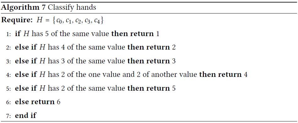
Hint: For the more general poker-hand identification, it can help to sort the values into ascending order. For this simplified algorithm, it helps to convert the list into a Counter object and examine the frequencies of the various card ranks. The Counter class is defined in the collections module with many other useful collection classes.

Each of the hands can be recognized by a function of the form:

    def hand_flavor(cards: Sequence[int]) -> bool: 
        examine the cards

This lets us write each individual hand-detection algorithm separately. We can then test them in isolation. This gives us confidence the overall hand classifier will work. It means you’ll need to write test cases on the individual classifiers to be sure they work properly.

4.9.3 Replace legs() with pairwise()

In the Pairing up items from a sequence section, we looked at the design for a legs() function to create pairs of legs from a sequence of waypoints.

This function can be replaced with itertools.pairwise(). After making this change, determine which implementation is faster.

4.9.4 Expand legs() to include processing

In the Pairing up items from a sequence section, we looked at the design for a legs() function to create pairs of legs from a sequence of waypoints.

A design alternative is to incorporate a function into the processing of legs() to perform a computation on each pair that’s created.

The function might look the following:

RT = TypeVar("RT") 
 
def legs(transform: Callable[[LL_Type, LL_Type], RT], lat_lon_iter: Iterator[LL_Type]) -> Iterator[RT]: 
    begin = next(lat_lon_iter) 
    for end in lat_lon_iter: 
        yield transform(begin, end) 
        begin = end

This changes the design of subsequent examples. Follow this design change through subsequent examples to see if this leads to simpler, easier-to-understand Python function definitions.