13.1 Downloading and installing

The PyMonad package is available on the Python Package Index (PyPI). In order to add PyMonad to your environment, you’ll need to use the python -m pip pymonad command to install it.

Once the PyMonad package is installed, you can confirm it using the following commands:

>>> import pymonad 
>>> help(pymonad)

This will display the module’s docstring and confirm that things really are properly installed.

The overall project name, PyMonad, uses mixed case. The installed Python package name that we import, pymonad, is all lower case.

13.2 Functional composition and currying

Some functional languages work by transforming a multi-argument function syntax into a collection of single argument functions. This process is called currying: it’s named after logician Haskell Curry, who developed the theory from earlier concepts. We’ve looked at currying in depth in Chapter 11, The Toolz Package. We’ll revisit it from the PyMonad perspective here.

Currying is a technique for transforming a multi-argument function into higher-order single argument functions. In a simple case, consider a function f(x,y) → z; given two arguments x and y; this will return some resulting value, z. We can curry the function f(x,y) into into two functions: f_c1(x) → f_c2(y) and f_c2(y) → z. Given the first argument value, x, evaluating the function f_c1(x) returns a new one-argument function, f_c2(y). This second function can be given the second argument value, y, and it returns the desired result, z.

We can evaluate a curried function in Python with concrete argument values as follows: f_c1(2)(3). We apply the curried function to the first argument value of 2, creating a new function. Then, we apply that new function to the second argument value of 3.

Let’s look at a concrete example in Python. For example, we have a function like the following one:

from pymonad.tools import curry  # type: ignore[import] 
 
@curry(4)  # type: ignore[misc] 
def systolic_bp( 
    bmi: float, age: float, gender_male: float, treatment: float 
) -> float: 
    return ( 
        68.15 + 0.58 * bmi + 0.65 * age + 0.94 * gender_male + 6.44 * treatment 
    )

This is a simple, multiple-regression-based model for systolic blood pressure. This predicts blood pressure from body mass index (BMI), age, gender (a value of 1 means male), and history of previous treatment (a value of 1 means previously treated). For more information on the model and how it’s derived, visit http://sphweb.bumc.bu.edu/otlt/MPH-Modules/BS/BS704_Multivariable/BS704_Multivariable7.html.

We can use the systolic_bp() function with all four arguments, as follows:

>>> systolic_bp(25, 50, 1, 0) 
116.09 
 
>>> systolic_bp(25, 50, 0, 1) 
121.59

A male person with a BMI of 25, age 50, and no previous treatment is predicted to have a blood pressure near 116. The second example shows a similar woman with a history of treatment who will likely have a blood pressure of 121.

Because we’ve used the @curry decorator, we can create intermediate results that are similar to partially applied functions. Take a look at the following command snippet that creates a new function, treated():

>>> treated = systolic_bp(25, 50, 0)
>>> treated(0)
115.15
>>> treated(1)
121.59

In the preceding case, we evaluated the systolic_bp(25, 50, 0) expression to create a curried function and assigned this to the treated variable. This built a new function, treated, with values for some of the parameters. The BMI, age, and gender values don’t typically change for a given patient. We can now apply the new treated() function to the remaining argument value to get different blood pressure expectations based on patient history.

Here’s an example of creating some additional curried functions:

>>> g_t = systolic_bp(25, 50) 
>>> g_t(1, 0) 
116.09 
>>> g_t(0, 1) 
121.59

This is a gender-based treatment function based on our initial model. We must provide both the needed gender and treatment argument values to get a final value from the model.

This is similar in some respects to the functools.partial() function. The important difference is that currying creates a function that can work in a variety of ways. The functools.partial() function creates a more specialized function that can only be used with the given set of bound values. For more information, see Chapter 10, The Functools Module.

>>> from pymonad.tools import curry 
>>> from functools import reduce 
 
>>> creduce = curry(2, reduce)

>>> from operator import add 
 
>>> my_sum = creduce(add) 
>>> my_sum([1,2,3]) 
6

>>> my_max = creduce(lambda x,y: x if x > y else y) 
>>> my_max([2,5,3]) 
5

import operator 
 
prod = creduce(operator.mul)

from collections.abc import Iterable 
 
@curry(1)  # type: ignore[misc] 
def alt_range(n: int) -> Iterable[int]: 
    if n == 0: 
        return range(1, 2)  # Only the value [1] 
    elif n % 2 == 0: 
        return range(2, n+1, 2)  # Even 
    else: 
        return range(1, n+1, 2)  # Odd

>>> prod(alt_range(9)) 
945

>>> from pymonad.reader import Compose 
>>> semi_fact = Compose(alt_range).then(prod) 
>>> semi_fact(9) 
945

13.3 Functors – making everything a function

The idea of a functor is a functional representation of a piece of simple data. A functor version of the number 3.14 is a function of zero arguments that returns this value. Consider the following example:

>>> pi = lambda: 3.14 
>>> pi() 
3.14

We created a zero-argument lambda object that returns a Python float object.

When we apply a curried function to a functor, we’re creating a new curried functor. This generalizes the idea of applying a function to an argument to get a value by using functions to represent the arguments, the values, and the functions themselves.

Once everything in our program is a function, then all processing becomes a variation on the theme of functional composition. To recover the underlying Python object, we can use the value attribute of a functor object to get a Python-friendly, simple type that we can use in uncurried code.

Since this kind of programming is based on functional composition, no calculation needs to be done until we actually demand a value using the value attribute. Instead of performing a lot of intermediate calculations, our program defines intermediate complex objects that can produce a value when requested. In principle, this composition can be optimized by a clever compiler or runtime system.

In order to work politely with functions that have multiple arguments, PyMonad offers a to_arguments() method. This is a handy way to clarify the argument value being provided to a curried function. We’ll see an example of this below, after introducing the Maybe and Just monads.

We can wrap a Python object with a subclass of the Maybe monad. The Maybe monad is interesting, because it gives us a way to deal gracefully with missing data. The approach we used in Chapter 12, Decorator Design Techniques, was to decorate built-in functions to make them None-aware. The approach taken by the PyMonad library is to decorate the data to distinguish something that’s just an object from nothing.

There are two subclasses of the Maybe monad:

• Nothing

• Just( some Python object )

We use Nothing similarly to the Python value of None. This is how we represent missing data. We use Just() to wrap all other Python objects. These are also functors, offering function-like representations of constant values.

We can use a curried function with these Maybe objects to tolerate missing data gracefully. Here’s a short example:

>>> from pymonad.maybe import Maybe, Just, Nothing 
 
>>> x1 = Maybe.apply(systolic_bp).to_arguments(Just(25), Just(50), Just(1), Just(0)) 
>>> x1.value 
116.09 
 
>>> x2 = Maybe.apply(systolic_bp).to_arguments(Just(25), Just(50), Just(1), Nothing) 
>>> x2 
Nothing 
>>> x2.value is None 
True

This shows us how a monad can provide an answer instead of raising a TypeError exception. This can be very handy when working with large, complex datasets in which data could be missing or invalid.

13.3.1 Using the lazy ListMonad() monad

The ListMonad() monad can be confusing at first. It’s extremely lazy, unlike Python’s built-in list type. When we evaluate the a list(range(10)) expression, the list() function will evaluate the range() object to create a list with 10 items. The PyMonad ListMonad() monad, however, is too lazy to even do this evaluation.

Here’s the comparison:

>>> list(range(10)) 
[0, 1, 2, 3, 4, 5, 6, 7, 8, 9] 
 
>>> from pymonad.list import ListMonad 
>>> ListMonad(range(10)) 
[range(0, 10)]

The ListMonad() monad did not evaluate the range() object’s iterable sequence of values; it preserved it without being evaluated. A ListMonad() monad is useful for collecting functions without evaluating them.

We can evaluate the ListMonad() monad later as required:

>>> from pymonad.list import ListMonad 
 
>>> x = ListMonad(range(10)) 
>>> x 
[range(0, 10)] 
>>> x[0] 
range(0, 10) 
>>> list(x[0]) 
[0, 1, 2, 3, 4, 5, 6, 7, 8, 9]

We created a lazy ListMonad() object which contained a range() object. Then we extracted and evaluated a range() object at position 0 in that list.

A ListMonad() object won’t evaluate a generator function. It treats any iterable argument as a single iterator object. We can, later, apply the function being contained by the monad.

Here’s a curried version of the range() function. This has a lower bound of 1 instead of 0. It’s handy for some mathematical work because it allows us to avoid the complexity of the positional arguments in the built-in range() function:

from collections.abc import Iterator 
from pymonad.tools import curry 
 
@curry(1)  # type: ignore[misc] 
def range1n(n: int) -> range: 
    if n == 0: return range(1, 2)  # Only the value 1 
    return range(1, n+1)

We wrapped the built-in range() function to make it curryable by the PyMonad package.

Since a ListMonad object is a functor, we can map functions to the ListMonad object. The function is applied to each item in the ListMonad object.

Here’s an example:

>>> from pymonad.reader import Compose 
>>> from pymonad.list import ListMonad 
 
>>> fact = Compose(range1n).then(prod) 
>>> seq1 = ListMonad(*range(20)) 
 
>>> f1 = seq1.map(fact) 
>>> f1[:10] 
[1, 1, 2, 6, 24, 120, 720, 5040, 40320, 362880]

We defined a composite function, fact(), which was built from the prod() and range1n() functions shown previously. This is the factorial function. We created a ListMonad() functor, seq1, which is a sequence of 20 values. We mapped the fact() function to the seq1 functor, which created a sequence of factorial values, f1. Finally, we extracted the first 10 of these values.

Here’s another little function that we’ll use to extend this example:

from pymonad.tools import curry 
 
@curry(1)  # type: ignore[misc] 
def n21(n: int) -> int: 
    return 2*n+1

This little n21() function does a simple computation. It’s curried, however, so we can apply it to a functor such as a ListMonad() object. Here’s the next part of the preceding example:

>>> semi_fact = Compose(alt_range).then(prod) 
>>> f2 = seq1.map(n21).then(semi_fact) 
>>> f2[:10] 
[1, 3, 15, 105, 945, 10395, 135135, 2027025, 34459425, 654729075]

We’ve defined a composite function from the prod() and alt_range() functions shown previously. The value of the f2 object is built by mapping our small n21() function applied to the seq1 sequence. This creates a new sequence. We then applied the semi_fact() function to each object in this new sequence to create a sequence of values that are parallels to the f1 sequence of values.

We can now map the / operator, operator.truediv, to these two parallel sequences of values, f1 and f2:

>>> import operator 
>>> 2 * sum(map(operator.truediv, f1, f2)) 
3.1415919276751456

The built-in map() function will apply the given operator to both functors, yielding a sequence of fractions that we can add.

We defined a fairly complex calculation using a few functional composition techniques and a functor class definition. This is based on a computation for the arctangent. Here’s the full definition for this calculation:

Ideally, we prefer not to use a fixed-size ListMonad object with only twenty values. We’d prefer to have a lazy and potentially infinite sequence of integer values, allowing us an approximation of arbitrary accuracy. We could then use curried versions of the sum() and takewhile() functions to find the sum of values in the sequence until the values are too small to contribute to the result.

This rewrite to use the takewhile() function is left as an exercise for the reader.

13.4 Monad bind() function

The name of the PyMonad library comes from the functional programming concept of a monad, a function that has a strict order. The underlying assumption behind much functional programming is that functional evaluation is liberal: it can be optimized or rearranged as necessary. A monad provides an exception that imposes a strict left-to-right order.

Python, as we have seen, is already strict. It doesn’t require monads. We can, however, still apply the concept in places where it can help clarify a complex algorithm. We’ll look at an example, below, of using a monad-based approach to designing a simulation based on Markov chains.

The technology for imposing strict evaluation is a binding between a monad and a function that will return a monad. A flat expression will become nested bindings that can’t be reordered by an optimizing compiler. The then() method of a monad imposes this strict ordering.

In other languages, such as Haskell, a monad is crucial for file input and output where strict ordering is required. Python’s imperative mode is much like a Haskell do block, which has an implicit Haskell >>= operator to force the statements to be evaluated in order. PyMonad uses the then() method for this binding.

13.5 Implementing simulation with monads

Monads are expected to pass through a kind of pipeline: a monad will be passed as an argument to a function and a similar monad will be returned as the value of the function. The functions must be designed to accept and return similar structures.

We’ll look at a monad-based pipeline that can be used for simulation of a process. This kind of simulation is sometimes called a Monte Carlo simulation. In this case, the simulation will create a Markov chain.

A Markov chain is a model for a series of potential events. The probability of each event depends only on the state attained in the previous event. Each state of the overall system had a set of probabilities that define the events and related state changes. It fits well with games that involve random chance, like dice or cards. It also fits well with industrial processes where small random effects can ”ripple through” the system, leading to effects that may not appear to be—directly—related to tiny initial problems.

Our example involves some rules for a fairly complex simulation. We can visualize the following state changes shown in Figure 13.1 as creating a chain of events that ends with either a Pass or Fail event. The number of events has a lower bound of 1.

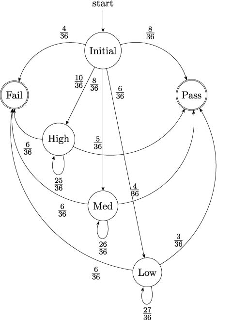
The state transition probabilities are stated as fractions, , because this particular Markov chain generator comes from a game that uses two dice. There are 36 possible outcomes from a roll of the dice. When considering the sum of the two dice, the 10 distinct values have probabilities ranging from for the values 2 and 12, to for the value 7.

Because this is based on a game, the actual algorithm is somewhat simpler than the diagram of the state transitions. The trick in simplifying the algorithm description is combining a number of similar behaviors into a single state defined by a parameter, p.

The algorithm’s use of an internal state. For designers new to functional programming, this is a bit of a problem. The solution that we’ve shown in other examples is to expose the state as a parameter to a function.

We’ll start with a presentation of the algorithm with explicit state.

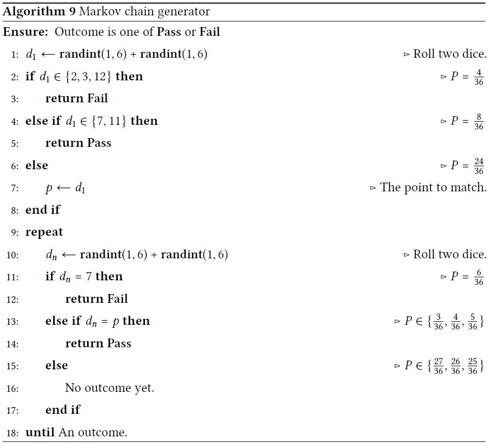
The algorithm can be seen as requiring a state change. Alternatively, we can look at this as a sequence of operations to append to the Markov chain, rather than a state change. There’s one function that must be used first to create an initial outcome or establish the value of p. Another, recursive function is used after that to iterate until an outcome is determined. In this way, this pairs-of-functions approach fits the monad design pattern nicely.

To build Markov chains, we’ll need a source of random numbers:

import random 
 
def rng() -> tuple[int, int]: 
    return (random.randint(1,6), random.randint(1,6)) 
 
from collections.abc import Callable 
from typing import TypeAlias 
 
DiceT: TypeAlias = Callable[[], tuple[int, int]]

The preceding function will generate a pair of dice for us. We also included a type hint, DiceT, that can be used to describe any similar function that returns a tuple with two integers. The type hint will be used in later functions as a shorthand for any similar random number generator.

Here’s our expectations from the overall chain generator based on the game algorithm:

from pymonad.maybe import Maybe, Just 
 
def game_chain(dice: DiceT) -> Maybe: 
    outcome = ( 
        Just(("", 0, [])) 
        .then(initial_roll(dice)) 
        .then(point_roll(dice)) 
    ) 
    return outcome

We create an initial monad, Just(("", 0, [])), to define the essential type we’re going to work with. A game will produce a three-tuple with the outcome text, the point value, and a sequence of rolls. At the start of each game, a default three-tuple establishes the three-tuple type.

We pass this monad to two other functions. This will create a resulting monad, outcome, with the results of the game. We use the then() method to connect the functions in the specific order they must be executed. In a language with an optimizing compiler, this will prevent the expression from being rearranged.

We will get the value of the monad at the end using the value attribute. Since the monad objects are lazy, this request is what triggers the evaluation of the various monads to create the required output.

Each resulting sequence of three-tuples is a Markov chain we can analyze to determine the overall statistical properties. We’re often interested in the expected lengths of the chains. This can be difficult to predict from the initial model or the algorithm.

The initial_roll() function has the rng() function curried as the first argument. The monad will become the second argument to this function. The initial_roll() function can roll the dice and apply the come out rule to determine if we have a pass, a fail, or a point.

The point_roll() function also has the rng() function curried as the first argument. The monad will become the second argument. The point_roll() function can then roll the dice to see if the game is resolved. If the game is unresolved, this function will operate recursively to continue looking for a resolution.

The initial_roll() function looks like this:

from pymonad.tools import curry 
from pymonad.maybe import Maybe, Just 
 
@curry(2)  # type: ignore[misc] 
def initial_roll(dice: DiceT, status: Maybe) -> Maybe: 
    d = dice() 
    if sum(d) in (7, 11): 
        return Just(("pass", sum(d), [d])) 
    elif sum(d) in (2, 3, 12): 
        return Just(("fail", sum(d), [d])) 
    else: 
        return Just(("point", sum(d), [d]))

The dice are rolled once to determine if the initial outcome is pass, fail, or establish the point. We return an appropriate monad value that includes the outcome, a point value, and the roll of the dice that led to this state. The point values for an immediate pass and immediate fail aren’t really meaningful. We could sensibly return a 0 value here, since no point was really established.

The point_roll() function looks like this:

from pymonad.tools import curry 
from pymonad.maybe import Maybe, Just 
 
@curry(2)  # type: ignore[misc] 
def point_roll(dice: DiceT, status: Maybe) -> Maybe: 
    prev, point, so_far = status 
    if prev != "point": 
        # won or lost on a previous throw 
        return Just(status) 
 
    d = dice() 
    if sum(d) == 7: 
        return Just(("fail", point, so_far+[d])) 
    elif sum(d) == point: 
        return Just(("pass", point, so_far+[d])) 
    else: 
        return ( 
            Just(("point", point, so_far+[d])) 
            .then(point_roll(dice)) 
        )

We decomposed the status monad into the three individual values of the tuple. We could have used small lambda objects to extract the first, second, and third values. We could also have used the operator.itemgetter() function to extract the tuple’s items. Instead, we used multiple assignment.

If a point was not established, the previous state will be pass or fail. The game was resolved during the initial_roll() function, and this function simply returns the status monad.

If a point was established, the state will be point. The dice is rolled and rules applied to this new roll. If roll is 7, the game is a lost and a final monad is returned. If the roll is the point, the game is won and the appropriate monad is returned. Otherwise, a slightly revised monad is passed to the point_roll() function. The revised status monad includes this roll in the history of rolls.

A typical output looks like this:

>>> game_chain() 
(’fail’, 5, [(2, 3), (1, 3), (1, 5), (1, 6)])

The final monad has a string that shows the outcome. It has the point that was established and the sequence of dice rolls leading to the final outcome.

We can use simulation to examine different outcomes to gather statistics on this complex, stateful process. This kind of Markov-chain model can reflect a number of odd edge cases that lead to surprising distributions of results.

A great deal of clever Monte Carlo simulation can be built with a few simple, functional programming design techniques. The monad, in particular, can help to structure these kinds of calculations when there are complex orders or internal states.

13.6 Additional PyMonad features

One of the other features of PyMonad is the confusingly named monoid. This comes directly from mathematics and it refers to a group of data elements that have an operator and an identity element, and the group is closed with respect to that operator. Here’s an example of what this means: when we think of natural numbers, the add operator, and an identity element 0, this is a proper monoid. For positive integers, with an operator *, and an identity value of 1, we also have a monoid; strings using + as an operator and an empty string as an identity element also qualify.

PyMonad includes a number of predefined monoid classes. We can extend this to add our own monoid class. The intent is to limit a compiler to certain kinds of optimization. We can also use the monoid class to create data structures which accumulate a complex value, perhaps including a history of previous operations.

The pymonad.list is an example of a monoid. The identity element is an empty list, defined by ListMonad(). The addition operation defines list concatenation. The monoid is an aspect of the overall ListMonad() class.

Much of this package helps provide deeper insights into functional programming. To paraphrase the documentation, this is an easy way to learn about functional programming in, perhaps, a slightly more forgiving environment. Rather than learning an entire language and toolset to compile and run functional programs, we can just experiment with interactive Python.

Pragmatically, we don’t need too many of these features because Python is already stateful and offers strict evaluation of expressions. There’s no practical reason to introduce stateful objects in Python, or strictly ordered evaluation. We can write useful programs in Python by mixing functional concepts with Python’s imperative implementation. For that reason, we won’t delve more deeply into PyMonad.

13.7 Summary

In this chapter, we looked at how we can use the PyMonad library to express some functional programming concepts directly in Python. The module contains many important functional programming techniques.

We looked at the idea of currying, a function that allows combinations of arguments to be applied to create new functions. Currying a function also allows us to use functional composition to create more complex functions from simpler pieces. We looked at functors that wrap simple data objects to make them into functions that can also be used with functional composition.

Monads are a way to impose a strict evaluation order when working with an optimizing compiler and lazy evaluation rules. In Python, we don’t have a good use case for monads because Python is an imperative programming language under the hood. In some cases, imperative Python may be more expressive and succinct than a monad construction.

In the next chapter, we’ll look at the multiprocessing and multithreading techniques that are available to us. These packages become particularly helpful in a functional programming context. When we eliminate a complex shared state and design around non-strict processing, we can leverage parallelism to improve the performance.

13.8 Exercises

This chapter’s exercises are based on code available from Packt Publishing on GitHub. See https://github.com/PacktPublishing/Functional-Python-Programming-3rd-Edition.

In some cases, the reader will notice that the code provided on GitHub includes partial solutions to some of the exercises. These serve as hints, allowing the reader to explore alternative solutions.

In many cases, exercises will need unit test cases to confirm they actually solve the problem. They are often identical to the unit test cases provided in the GitHub repository. The reader should replace the book’s example function name with their own solution to confirm that it works.

13.8.2 Statistical computations

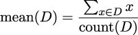
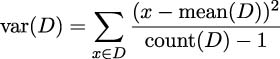
Given a list of values, v, we can create a useful monad with Just(v). We can use built-in functions like sum() and len() with the Just.map() method to compute the values required for mean, variance, and standard deviation.

After implementing these functions using PyMonad, compare these definitions with more conventional Python language techniques. Does the presence of a monad structure help with these relatively simple computations?