
24
Approximate Bayesian Inference Using the Mean-Field Distribution
Dynamical systems representing populations of interacting heterogeneous individuals are rarely studied and validated within a Bayesian framework, with the notable exception of Schneider et al. (2006), dealing with a model of plants in competition for a light resource. The reasons for this lack of coverage of a subject with such significant stakes (agriculture, crowd dynamics) are to be found in the computational difficulties posed by the problem of inference when the size of the population is large. In this chapter, we will focus on dynamical systems admitting a mean-field limit distribution when the population’s size tends to infinity, such as the flocking models presented in Carrillo et al. (2010). We introduce a numerical scheme to simulate the mean-field distribution, which is a partial differential transport equation solution, and we use these simulations to simplify the likelihood distributions associated with Bayesian inference problems arising when the population is only partially observed.
24.1. Introduction
Population models may be used to assess, from data, the interaction laws governing the individual dynamics (Bongini et al. 2017; Lu et al. 2019). In most of these models, the interaction of an individual with the rest of the population is represented by means of some statistics, potentially depending on the state variables of the whole population. These statistics can take the form of the average velocity in birds swarms, for example, (Cucker and Smale 2007; Degond et al. 2014), or the mean competition potential exerted by a population of plants over a single plant in Schneider et al. (2006). In this chapter, we will consider population models that satisfy a list of frequently encountered properties:
- – Each individual in the population is represented by a state variable x, which may vary through time, and an individual trait variable θ, which remains constant. The variability of trait θ from one individual to another can be used to model the heterogeneous aspect of the population.
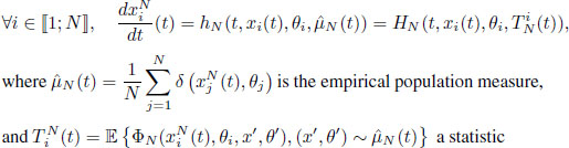
- – The evolution of a population of N individuals is given by a differential system, where the motion of each individual i is driven by a transition function hN depending on some population statistics
 , i.e. for any time t ≥ 0,
defined with ![]() a feature function.
a feature function.
In the above equation, we have used the notation δ(x, θ) for the Dirac distribution centered at point (x, θ). The empirical population measure ![]() is the probability distribution corresponding to the uniform sampling of an individual (x, θ) in the population.
is the probability distribution corresponding to the uniform sampling of an individual (x, θ) in the population. ![]() is used to compute all possible statistics over the population, such as the first-order moment and covariance of the state variable. Here we consider statistics taking a form expressed as the empirical expectation of the function ΦN. The state variable x evolves in an Euclidean space
is used to compute all possible statistics over the population, such as the first-order moment and covariance of the state variable. Here we consider statistics taking a form expressed as the empirical expectation of the function ΦN. The state variable x evolves in an Euclidean space ![]() , while the individual trait θ remains within a finite-dimensional metric space Θ.
, while the individual trait θ remains within a finite-dimensional metric space Θ.
- – To account for the uncertainty on the initial configuration of the system, the collection of initial conditions and individual traits
 is assumed to be an independent and identically distributed (i.i.d.) sample of some distribution
  , referred to as the initial distribution.
When the initial distribution is factorized and when the transition function depends, as above, on the empirical measure ![]() , then the system dynamics has the property of being invariant by permutation of its individuals’ labels. We then say that the system is symmetric if for any time t ≥ 0 and for any bijection ρ: 〚1; N〛 → 〚1; N〛 , the distribution of the permuted collection (xρ(1:N)(t), θρ(1:N)) is the same as the original collection (x1:N(t), θ1:N). This property is commonly shared by population models, where, most often, the assignment of labels is arbitrary (Carrillo et al. 2010).
, then the system dynamics has the property of being invariant by permutation of its individuals’ labels. We then say that the system is symmetric if for any time t ≥ 0 and for any bijection ρ: 〚1; N〛 → 〚1; N〛 , the distribution of the permuted collection (xρ(1:N)(t), θρ(1:N)) is the same as the original collection (x1:N(t), θ1:N). This property is commonly shared by population models, where, most often, the assignment of labels is arbitrary (Carrillo et al. 2010).
Our focus in this chapter is to discuss the statistical inference problems related to the study of such symmetric systems. More specifically, when some elements of the structure of the system are partially known, such as the initial condition or the size N of the population, determining parameters of the transition function hN or the initial distribution μ0 can appear as a very complex task, leading to the necessity of building approximations. In section 24.2, the plant population model introduced by Schneider et al. (2006) is taken as an example of systems leading to difficult inference problems when the size of the population is partially known. Section 24.3 uses an asymptotic property of the empirical measure of the Schneider system when N → ∞, i.e. the fact that it admits a mean-field limit distribution, to simplify the previously mentioned inference problem. Section 24.4 deals with the consistency of this approximation.
24.2. Inference problem in a symmetric population system
24.2.1. Example of a symmetric system describing plant competition
In this section, we consider a plant growth model with competition, first introduced by Schneider et al. (2006) and later by Lv et al. (2008) and Nakagawa et al. (2015). This system describes the growth of Arabidopsis thaliana: each plant is represented by the state variable ![]() , the diameter of its rosette, its position
, the diameter of its rosette, its position ![]() and two growth parameters
and two growth parameters ![]() , namely, the growth rate and the asymptotic isolated size. As the parameters x, S, γ remain constant over time, they are considered as components of the individual trait θ. The differential system giving the dynamics of N plants takes the following expression, for all plant i ∈ 〚1; N〛 and for all t ≥ 0,
, namely, the growth rate and the asymptotic isolated size. As the parameters x, S, γ remain constant over time, they are considered as components of the individual trait θ. The differential system giving the dynamics of N plants takes the following expression, for all plant i ∈ 〚1; N〛 and for all t ≥ 0,
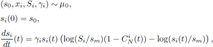
where sm > 0 is a minimal size parameter and

In the equation above, ![]() models the competition exerted on plant i by all the other plants at time t. As we can read in the competition potential C(si(t), sj (t), |xi − xj|), the competition is stronger the closer the competitors are to plant i and larger they are in relation to plant i. We assume that the distribution μ0 is such that all plants initially have the same size s0 > sm. RM, σx and σr are parameters of the competition potential. Because this system is nonlinear, we need to make additional assumptions on the initial distribution μ0 to ensure that the system has a biologically consistent behavior, in particular, that a finite-time blowup cannot occur, or that the competition potential does not take negative values. A sufficient condition to prevent such pathological situations from appearing is to include the support of the initial distribution μ0 within the domain
models the competition exerted on plant i by all the other plants at time t. As we can read in the competition potential C(si(t), sj (t), |xi − xj|), the competition is stronger the closer the competitors are to plant i and larger they are in relation to plant i. We assume that the distribution μ0 is such that all plants initially have the same size s0 > sm. RM, σx and σr are parameters of the competition potential. Because this system is nonlinear, we need to make additional assumptions on the initial distribution μ0 to ensure that the system has a biologically consistent behavior, in particular, that a finite-time blowup cannot occur, or that the competition potential does not take negative values. A sufficient condition to prevent such pathological situations from appearing is to include the support of the initial distribution μ0 within the domain
In other words, the initial size is lower than the asymptotic isolated size S, and the asymptotic size is below some threshold depending on the competition parameter RM. In this setting, we can prove that for all i ∈ 〚1; N〛 , and for all t ≥ 0, sm ≤ si(t) ≤ Si and that ![]() almost surely, which is consistent with the initial assumptions of the model. Indeed, for any time t > 0 sufficiently close to zero, we have the following inequality on the derivative of the state variable:
almost surely, which is consistent with the initial assumptions of the model. Indeed, for any time t > 0 sufficiently close to zero, we have the following inequality on the derivative of the state variable:
which leads to ![]() and that proves that the inequality sm ≤ si(t) ≤ Si holds for any time
and that proves that the inequality sm ≤ si(t) ≤ Si holds for any time ![]() .
.
The Schneider system fits into the definition of symmetric population models as the transition function can be expressed as a function of the individual variables and the population empirical measure only. The differential system can be rewritten as follows:
where ![]()
and ![]()
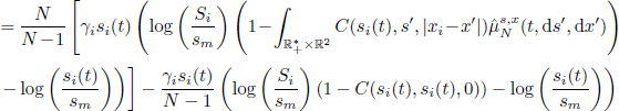
In the equation above, we use the notation ![]() to denote the marginal distribution of distribution
to denote the marginal distribution of distribution ![]() with respect to the variables s, x. The second term in the expression of hN represents the exclusion of the diagonal interaction, between an individual plant and itself.
with respect to the variables s, x. The second term in the expression of hN represents the exclusion of the diagonal interaction, between an individual plant and itself.
Now that we have guarantees on the global existence of the trajectories of the Schneider system, we can consider a numerical methodology to estimate the evolution of individual sizes ![]() . The numerical scheme we introduce in this chapter takes into account the two-level structure of the dynamics: a population level represented by the competition potential
. The numerical scheme we introduce in this chapter takes into account the two-level structure of the dynamics: a population level represented by the competition potential ![]() and an individual level represented by variables (si, θi). Let {t0 = 0, t1, …, tM = T} be a subdivision of the interval [0; T], over which we want to simulate the system. Then, over each time instance of this sub-interval [tk ; tk+1), for k ∈ 〚0; M − 1〛 , we approximate the evolution of each individual competition potential by a piecewise polynomial function, given by a Taylor expansion with respect to time variable t:
and an individual level represented by variables (si, θi). Let {t0 = 0, t1, …, tM = T} be a subdivision of the interval [0; T], over which we want to simulate the system. Then, over each time instance of this sub-interval [tk ; tk+1), for k ∈ 〚0; M − 1〛 , we approximate the evolution of each individual competition potential by a piecewise polynomial function, given by a Taylor expansion with respect to time variable t:
With this approximation, we can obtain an approximation of the individual trajectories over the interval [tk; tk+1) by solving the analytical differential equation for all i ∈ 〚1; N〛 :
![]() given by the previous iteration,
given by the previous iteration,
After this, we can evaluate the competition potentials ![]() at the next time
at the next time
24.2.2. Inference problem of the Schneider system, in a more general setting
Let us consider the inference problem consisting of the identification of parameters ![]() from observations made on a sub-population of size N0 ≤ N. The actual size N of the population is unknown; it is a latent variable of the problem. We introduce the prior distributions pη, pN on the parameters to estimate and on the unknown size, respectively. We consider that the support of the prior pN is infinite, included in the interval 〚N0; +∞〚. Let us assume that the observation error is Gaussian of standard deviation σ, and that observations are made independently over the timeline
from observations made on a sub-population of size N0 ≤ N. The actual size N of the population is unknown; it is a latent variable of the problem. We introduce the prior distributions pη, pN on the parameters to estimate and on the unknown size, respectively. We consider that the support of the prior pN is infinite, included in the interval 〚N0; +∞〚. Let us assume that the observation error is Gaussian of standard deviation σ, and that observations are made independently over the timeline ![]() . We denote by
. We denote by ![]() the random variable representing the observations, sij being the measured size of individual i at time tj. In a Bayesian setting, we would like to estimate the posterior distribution of η knowing the observations s. Bayes’ formula classically gives the following expression of the posterior density, which can only be known up to a multiplicative factor in our case, i.e. for all
the random variable representing the observations, sij being the measured size of individual i at time tj. In a Bayesian setting, we would like to estimate the posterior distribution of η knowing the observations s. Bayes’ formula classically gives the following expression of the posterior density, which can only be known up to a multiplicative factor in our case, i.e. for all ![]() ,
,
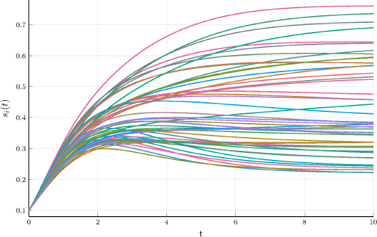
Figure 24.1. Evolution of plant sizes in a population of N = 50 individuals described by the Schneider system. All plants initially have the same size s0, and the individual traits θ = (x, S, γ) have a uniform distribution in a domain included within  . Trajectories are computed using the two-level numerical scheme introduced in the section. For a color version of this figure, see www.iste.co.uk/zafeiris/data1.zip
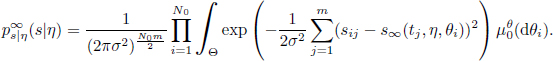
Beforehand, the inference requires the evaluation of the likelihood distribution ps|η of the observations knowing the parameters. The likelihood of the observations has a density ps|η of expression
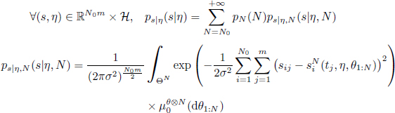
where ![]() is the solution of the Schneider system of size N. In practice, we cannot evaluate the trajectories
is the solution of the Schneider system of size N. In practice, we cannot evaluate the trajectories ![]() exactly, and we have to resort to numerical methods to estimate them. The management of this source of uncertainty is out of the scope of this chapter, and let us assume that we are able to solve the differential system exactly, or with a numerical error that we can reasonably ignore.
exactly, and we have to resort to numerical methods to estimate them. The management of this source of uncertainty is out of the scope of this chapter, and let us assume that we are able to solve the differential system exactly, or with a numerical error that we can reasonably ignore.
The main difficulty in the computation of this likelihood distribution comes from the fact that individuals are interdependent for any time t > 0. As a consequence, to compute the trajectory ![]() , we need to introduce the initial configuration of the whole population θ1:N as latent variables, although we only observe a subset of N0 individuals. Thus, the likelihood appears as an infinite mixture of densities, due to the infinite support of the prior pN. Moreover, each of the densities in the mixture is expressed as an integral over a space of increasing dimension. The inference problem associated with the simulation of a posterior distribution with a latent variable changing the dimension of the candidate model is called a trans-dimensional inference problem (Preston 1975). Numerically simulating such a complex distribution is still an open research topic, as pointed out in Roberts and Rosenthal (2006).
, we need to introduce the initial configuration of the whole population θ1:N as latent variables, although we only observe a subset of N0 individuals. Thus, the likelihood appears as an infinite mixture of densities, due to the infinite support of the prior pN. Moreover, each of the densities in the mixture is expressed as an integral over a space of increasing dimension. The inference problem associated with the simulation of a posterior distribution with a latent variable changing the dimension of the candidate model is called a trans-dimensional inference problem (Preston 1975). Numerically simulating such a complex distribution is still an open research topic, as pointed out in Roberts and Rosenthal (2006).
24.3. Properties of the mean-field distribution
To ignore the aforementioned source of uncertainty, we resort to the notion of mean-field limit distribution, which is used in statistical physics and in mathematical biology (Carrillo et al. 2010). This notion describes the asymptotic behavior of a population system, for which the population empirical measure ![]() converges weakly and almost surely, when N → ∞, towards some deterministic probability distribution μ(t), referred to as the mean-field distribution. The weak convergence of the sequence
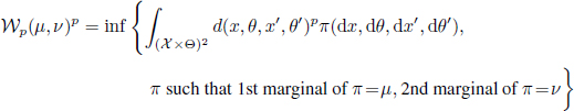
converges weakly and almost surely, when N → ∞, towards some deterministic probability distribution μ(t), referred to as the mean-field distribution. The weak convergence of the sequence ![]() is quantified classically by the Wasserstein distance (Golse 2016). It is formally defined for any couple of probability measures
is quantified classically by the Wasserstein distance (Golse 2016). It is formally defined for any couple of probability measures ![]() and for any p ≥ 1 by the infimum of the distance averaged by a coupling of the distributions μ and ν, i.e.
and for any p ≥ 1 by the infimum of the distance averaged by a coupling of the distributions μ and ν, i.e.
with d being some metric defined over ![]() . When a sequence of probability measure
. When a sequence of probability measure ![]() converges to some distribution μ for the metric
converges to some distribution μ for the metric ![]() , it means, in particular, that, for all φ continuous and bounded, we have
, it means, in particular, that, for all φ continuous and bounded, we have
and that the moments of order p of the sequence converge also towards the same moments of the limit distribution. In the case of the population empirical measure, this convergence can only hold almost surely, since ![]() is a stochastic measure depending on the initial configuration of the system.
is a stochastic measure depending on the initial configuration of the system.
As the empirical measure ![]() is a description of the population of size N, the limit μ(t) of this sequence can be interpreted as a description of an infinite population. The mean-field distribution μ(t) addresses the issues entailed by the interdependence of the individuals, since the individuals in this infinite population are independent. Such a paradox can be explained by comparing the interactions within a subgroup of individuals of constant size in a population of increasing N admitting a mean-field distribution. Let us illustrate this on a toy example.
is a description of the population of size N, the limit μ(t) of this sequence can be interpreted as a description of an infinite population. The mean-field distribution μ(t) addresses the issues entailed by the interdependence of the individuals, since the individuals in this infinite population are independent. Such a paradox can be explained by comparing the interactions within a subgroup of individuals of constant size in a population of increasing N admitting a mean-field distribution. Let us illustrate this on a toy example.
We consider a linear population model, given by
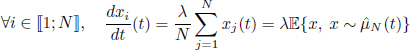
with Gaussian initial condition ![]() . The analytical trajectories of this system are for all i ∈ 〚1; N〛 and all t ≥ 0:
. The analytical trajectories of this system are for all i ∈ 〚1; N〛 and all t ≥ 0:
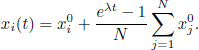
It is quite straightforward to prove that, in this case, the empirical measure has a mean-field limit, for any time t ≥ 0 and almost surely,
Besides, if we consider the covariance of two particles ![]() and
and ![]() , that are Gaussian,
, that are Gaussian,
It follows that these two particles are asymptotically independent. This property of asymptotic independence can be generalized to more complex and nonlinear systems, as long as they admit mean-field limits. In a symmetric system of the type in equation [24.1], a necessary condition for the existence of the mean-field limit is the pointwise convergence of the transition function hN when N → ∞. This pointwise convergence is clearly satisfied in the case of the toy example above, since we have, for any fixed probability measure ![]() , which is independent of N. It is also the case of the Schneider system, as we can see in equation [24.3], replacing
, which is independent of N. It is also the case of the Schneider system, as we can see in equation [24.3], replacing ![]() by a fixed probability measure μ. Moreover, we can prove the convergence
by a fixed probability measure μ. Moreover, we can prove the convergence ![]() almost surely for any t ≥ 0, where μ(t) is defined as the pushforward measure of the initial distribution μ0 by the flow of the following differential equation, starting from the initial configuration (s0, θ) = (s, x, S, γ),
almost surely for any t ≥ 0, where μ(t) is defined as the pushforward measure of the initial distribution μ0 by the flow of the following differential equation, starting from the initial configuration (s0, θ) = (s, x, S, γ),
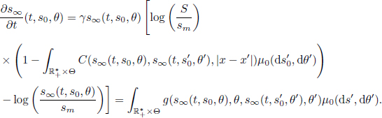
This equation can be interpreted as the continuous version of the original Schneider system, where the empirical expectation is replaced by the theoretical expectation. For all time t ≥ 0, the mean-field limit of the Schneider system is given by μ(t) = (s∞(t), IdΘ)#μ0, where # is the pushforward operator between a function and a probability measure. To prove the existence and uniqueness of the flow s∞, we proceed to the exact same steps as in the proof of the Cauchy–Lipschitz theorem, except that this time the initial conditions are not scalar but probability distributions. More specifically, the existence and uniqueness are consequences of a fixed point procedure, with the recurrence equation:
The sequence ![]() converges for some functional metric to a fixed point of the recurrence function, which defines the mean-field flow s∞. The convergence of the empirical measure
converges for some functional metric to a fixed point of the recurrence function, which defines the mean-field flow s∞. The convergence of the empirical measure ![]() is proved in Della Noce et al. (2019), resorting to an argument referred to as the propagation of chaos.
is proved in Della Noce et al. (2019), resorting to an argument referred to as the propagation of chaos.
24.4. Mean-field approximated inference
24.4.1. Case of systems admitting a mean-field limit
Let us return to the inference problem described in section 24.2.2. We consider the following approximation: if the size of the population is large enough, s∞ is close to the individual trajectories, and we can assume that observations are made on the infinite population rather than on the finite population. Under this approximation, the resulting likelihood of the observations has a simplified expression, in comparison with the original one in equation [24.4]:
Here, the asymptotic independence of the individuals is used to decompose the integral into a product of integrals over space Θ, the dimension of which does not depend on N. As a consequence of the convergence of the empirical measure mentioned in the previous section, we can prove that this approximation of the likelihood is consistent when N → ∞, and the convergence of the likelihood is quantified, in this case, using the total variation distance:

Moreover, the speed of the convergence towards the mean-field approximated inference depends on the configuration of the observation protocol, with an upper bound of the total variation distance taking the following expression:
which means that, for an accurate observation protocol (with large N0 and small σ), the mean-field approximation is relevant for population size N higher than in the case of a rough observation protocol.
We can therefore use this limit in total variation to approximate the infinite mixture of densities by a finite mixture, by truncating the infinite sum in equation [24.4] at a size N = Nmf, above which the mean-field likelihood is close to the original likelihood, below some tolerance ε
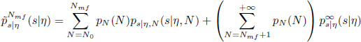
This approximated likelihood seems much more manageable than the original one. Nevertheless, the main difficulty is in the simulation of the mean-field flow s∞ which is used in the expression of ![]() .
.
To estimate the mean-field flow s∞, we use a two-level numerical method with the same structure as the numerical method used in section 2.1 to simulate a population of finite size N. Similarly, we consider the same subdivision {t0 = 0, t1,…, tM = T} of the interval [0; T]. In a finite population, the dynamics of the individuals’ sizes are driven by the competition potential ![]() , and, in the case of an infinite population, the same role is played by the averaged competition potential, defined for all
, and, in the case of an infinite population, the same role is played by the averaged competition potential, defined for all ![]() by
by
Over each sub-interval [tk ; tk+1) for k ∈ 〚1; M〛 , we approximate the C∞ by a piecewise polynomial function with respect to time and by a dense parametric family to approximate the dependency with respect to (s, θ) (we can choose multivariate polynomial functions if the domain of the variables is compact). The resulting approximation of C∞ over the interval takes the following form:
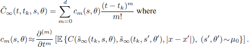
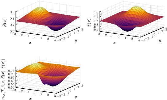
Figure 24.2. Top left: mean value of the parameter S according to the position x of the plant. Top right: mean value of the parameter γ according to the position of the plant. Bottom: evaluation of the mean-field flow s∞ at the end of the observation period, with the mean values of parameters S and γ. s∞ is computed using the two-level numerical scheme introduced in this section. For a color version of this figure, see www.iste.co.uk/zafeiris/data1.zip
Once the trajectories of the competition potential are approximated, we can analytically compute an approximation of the mean-field flow s∞ by solving a differential equation over [tk ; tk+1). The analytical differential equation to solve is

Figure 24.2 gives an illustration of simulations of the Schneider system under the mean-field approximation. We consider a specific initial distribution μ0 giving the parameters x, S, γ. We use the two-level numerical scheme introduced in this section to evaluate the numerical flow at a time T, where the individual sizes are close to a stationary distribution. We can note the impact of competition between the plants, as the surface corresponding to the mean-field flow does not entirely correspond to the surface characterizing the spatial distribution of parameter S.
24.5. Conclusion
In this chapter, we have presented a methodology to simplify inference problems related to symmetric systems admitting a mean-field distribution. This methodology should not be confused with the mean-field variational inference, which considers the minimization of other metrics to simplify the inference, most often the Kullback–Leibler divergence. The research on how to generalize such an approach to the symmetric system with less restrictive asymptotic behavior is ongoing.
24.6. References
Bongini, M., Fornasier, M., Hansen, M., Maggioni, M. (2017). Inferring interaction rules from observations of evolutive systems I: The variational approach. Mathematical Models and Methods in Applied Sciences, 27(05), 909–951.
Carrillo, J.A., Fornasier, M., Toscani, G., Vecil, F. (2010). Particle, kinetic, and hydrodynamic models of swarming. In Mathematical Modeling of Collective Behavior in Socio-Economic and Life Sciences, Naldi, G., Pareschi, L., Toscani, G. (eds). Birkhäuser, Boston.
Cucker, F. and Smale, S. (2007). On the mathematics of emergence. Japanese Journal of Mathematics, 2(1), 197–227.
Degond, P., Dimarco, G., Mac, T.B.N. (2014). Hydrodynamics of the Kuramoto–Vicsek model of rotating self-propelled particles. Mathematical Models and Methods in Applied Sciences, 24(02), 277–325.
Della Noce, A., Mathieu, A., Cournède, P.H. (2019). Mean field approximation of a heterogeneous population of plants in competition. arXiv preprint [Online]. Available at: arXiv:1906.01368.
Golse, F. (2016). On the dynamics of large particle systems in the mean field limit. In Macroscopic and Large Scale Phenomena: Coarse Graining, Mean Field Limits and Ergodicity, Muntean, A., Rademacher, J., Zagaris, A. (eds). Springer, Cham.
Lu, F., Zhong, M., Tang, S., Maggioni, M. (2019). Nonparametric inference of interaction laws in systems of agents from trajectory data. Proceedings of the National Academy of Sciences, 116(29), 14424–14433.
Lv, Q., Schneider, M.K., Pitchford, J.W. (2008). Individualism in plant populations: Using stochastic differential equations to model individual neighbourhood-dependent plant growth. Theoretical Population Biology, 74(1), 74–83.
Nakagawa, Y., Yokozawa, M., Hara, T. (2015). Competition among plants can lead to an increase in aggregation of smaller plants around larger ones. Ecological Modelling, 301, 41–53.
Preston, C. (1975). Spatial birth and death processes. Advances in Applied Probability, 7(3), 465–466.
Roberts, G.O. and Rosenthal, J.S. (2006). Harris recurrence of Metropolis-within-Gibbs and trans-dimensional Markov chains. The Annals of Applied Probability, 16(4), 2123–2139.
Schneider, M.K., Law, R., Illian, J.B. (2006). Quantification of neighbourhood-dependent plant growth by Bayesian hierarchical modelling. Journal of Ecology, 94, 310–321.
Chapter written by Antonin DELLA NOCE and Paul-Henry COURNÈDE.