
6
Forestry Logistics
| Heading |
Cooperative supply for forestry logistics | |
| Function/service |
Timber supply to primary processing sites | |
| Type of network Semantics of nodes and edges | □ sociological nodes: edges: | |
| Users (modes of inclusion) | □ circulating entities |
|
| Infrastructure | □ dedicated | |
| Intermediation | □ without operator | |
| Nature of flows |
□ continuous |
□ intangible
|
| Flow units |
Displaced mass (tons.km) | |
| Mode of transport | □ ambient | |
| Control |
□ load □ distributed | |
| Engineering issue |
| |
| Analysis tools |
| |
6.1. Summary of the study
The supply of primary timber processing industries (sawmills, paper industry) is traditionally provided by operators, each with their own resources (standing timber, means of logging and transportation) to meet the needs of their customers. Based on a real-world example, this study assesses the productivity gains that can be expected from the establishment of collaborative procurement methods. To do this, we use the tactical planning model for collaborative timber transport, which was developed in Moad (2016).
6.2. Forest timber supply problem
The supply of industrial sites that consume specific types of forest timber is subject to various availability constraints (species, volumes, quality), and the availability of handling and transport equipment.
The cut timber is stored on the roadside near the logging sites, in the form of stockpiles that are homogeneously stored according to species and quality. In the case of private forests, plots only produce a small volume of timber, creating a scattered and variable timber supply. In addition, efforts must be made to collect the cut timber quickly and avoid biotic health hazards by refraining from leaving any deposits in the forest (i.e. the remains of the stockpile).
The transport of timber is confronted by a VRP (vehicle routing planning) with a limited capacity type problem.
In this study, we deal with tactical procurement planning. This involves defining a plan for allocating timber sources to delivery sites, minimizing the overall movement of timber and taking into account the aggregate capacity of transport fleets.
First, we describe the planning model, adapted from Moad (2016) and François et al. (2017), with the aim of calculating a load plan for each transporter so as to:
- – minimize the overall displacement of timber;
- – minimize the number of loads;
- – reduce the activity duration (makespan) of each transporter;
- – regulate the level of stocks (depot specific to each transporter).
All this, while respecting business constraints, will:
- – avoid leaving stockpile remains in the forest;
- – prioritize the collection of timber with reference to a priority index (e.g. for biotic hazards).
Next, we apply the planning model to assess, according to a similar industrial case study, the productivity gains that can be obtained through a collaborative approach to the supply chain, rather than the collaborative activities of the transport carriers.
The following notations signify:
- – e: transport company;
- – s: loading site;
- – c: unloading site;
- – r: product reference;
- – t: activity plan period number;
- – Diss,c: distance from the loading site s to the unloading site c (km);
- – Demc,r: tonnage requested by the customer c for the product r (tons);
- – Invs,r,0: initial level of stock for product r at site s;
- – lTgc,r : target stock level for product r for depot c;
- – Gens,r,t: tonnage of product r generated on site s over the period t;
- – CT : truck transport capacity (tons);
- – Cape,t: aggregate capacity over period t by the company e (tons.km);
- – Cap’e,t: aggregate capacity over period t by the company e (tons).
6.3. Tactical planning model
The tactical planning model determines the allocation of collection points to delivery points. The decision is guided by a set of optimization penalties:
- – CTransport: penalty coefficient on the overall transport of timber;
- – CEmptying: penalty coefficient on the residual stockpile remains;
- – Prioritys,r: level of priority to collect product r from stockpile s;
- – CLoadings: penalty per number of loads;
- – CMakespane : penalty relating to the activity duration of the company e;
- – CInventory: penalty relating to deviations of stocks from a reference level (parameter ITgc,r).
The decision variables are:
- – Xe,s,c,r,t: tonnage of the product reference r transported from site s to site c by the company e over the period t (tons);
- – Invs,r,t : stock level of the product reference r at site s at the end of the period t;
- – Emps,r,t: Boolean variable equal to 0 if the stock s for the product reference r is empty at the end of the period t, or else equal to 1;
- – Acte,t: Boolean variable equal to 0 if the company e is inactive for a period t, or else equal to 1;
-
– NLe,c,r,t : number of deliveries of the product reference r by the company e to site c over the period t.
The objective function of the planning optimization problem is formulated as follows, minimize:
The components [6.1]–[6.5] of the objective function address, point by point, the tactical optimization problem described previously.
The constraints are as follows:
Equalities [6.6] ensure that the truck capacity is fully utilized. Equalities [6.7] guarantee satisfaction of the demand. The inequalities [6.8] express that the quantities taken from each stock do not exceed the quantities available. Equations [6.9] follow the evolution of stocks. The inequalities [6.10] and [6.11] guarantee that the load plan calculated for each company is compatible, for any period, with its aggregated capacity (in tons.km and tons). Finally, equations [6.12] and [6.13], where M is a sufficiently large real number, manage the instantiation of the Boolean variables of the model.
The objective function and constraints formulated above determine a linear optimization1 problem in terms of mixed-integer and Boolean variables. The solver used is CPLEX.
6.4. Logistics benchmarking
This involves comparing the logistics performance obtained according to two supply scenarios relating to a similar industrial case study. Starting from an existing “AS IS” scenario, we want to evaluate an improved “TO BE” scenario.
6.4.1. AS IS scenario (non-collaborative logistics)
The AS IS supply scenario is characterized by transport operators acting in complete independence; the customers, the timber sources and the means of transport are specific to each of the three carrier companies e1, e2, e3. We consider the activity of these companies over 5 days T1, … ,T5. The company e1 supplies the customer c1 with timber of two types P1, P2 extracted from forests at three sites s1, s2, s3. The transported timber is unloaded at the customer c1 or at the company’s own depot Dep1. Similarly, the other two companies each supply a customer from three loading points in the forest and their own depot (Figure 6.1). The data in square brackets indicate, by product, the tonnage of the available timber at the start of the week (start of period T1) in the various stocks (loading sites and depots), as well as the tonnage requested by each customer, to be delivered before the end of the week (end of period T5).
The daily aggregate transport capacity of each company, shown in Figure 6.2, results from the following data: the company e1 has two trucks, one of which is immobilized for maintenance on days T1 and T2. The company e2 has two trucks, while the company e3 has three trucks. The payload of the trucks is 37 tons and the daily activity of the drivers is limited to a 500 km cumulative journey with a maximum of six loads. The aggregate transport capacity Cape,t of a company e on a day t is therefore estimated at 18,500 tons.km multiplied by the number of trucks available. In addition, its aggregate transport capacity Cap’e,t is six loads of 37 tons, or 222 tons per truck available on day t.
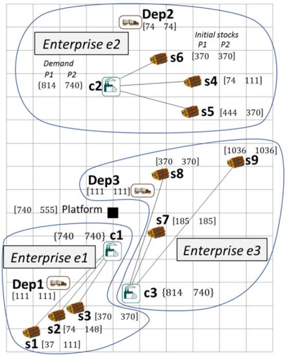
Figure 6.1. AS IS scenario: demand and inventory status at the start of the week. For a color version of this figure, see www.iste.co.uk/bourrieres/networks.zip
6.4.2. TO BE scenario (collaborative logistics)
Under the identical demand conditions, timber availability and transport capacity as the AS IS scenario, we propose here to determine an activity plan that takes advantage of timber and transport pooling. In this TO BE scenario, the transfer of timber from any source s1–s9 to any customer c1–c3 can be allocated to any transport company e1–e3. The contractual and transactional implications of the collaborative scenario remain implicit in this study.
6.4.3. Results
The scenarios are compared using the following performance indicators:
- – The minimum of the objective function, or the global score, which results from the sum of the components [6.1]–[6.5], themselves proportional to the penalty coefficients CTransport, CEmptying, CLoadings, CMakespane and CInventory. The minimization of the objective function reflects the supply policy.
- – The demand fulfillment rate: percentage of the demand actually delivered to the customers at the end of the 5th day.
- – The load rate of aggregate transport capacities, overall and by company, for each day of the delivery plan. This rate compares the planned activity to the available capacity, with reference to the movement of timber (in tons.km) or tonnage (in tons).
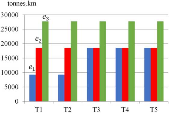
Figure 6.2. Aggregate transport capacity. For a color version of this figure, see www.iste.co.uk/bourrieres/networks.zip
The comparative results presented in Figures 6.3 and 6.4 are obtained by a significant weighting of the coefficient CEmptying, which reflects a strict policy to purge the remainder of the stockpile. The timber transports carried out by each of the transporters are shown in Figure 6.5. In this figure, the data in brackets [ ] indicate the initial state at the start of day 1, as well as the final state at the end of day 5, for the stockpiles in the forest for products P1 and P2. The data in brackets ( ) are the quantities of transported timber, and the data in brackets { } indicate the demand and the delivery made at the end of day 5. The colors are specific to each company.
The merits of the collaborative scenario are multiple. As shown in Figure 6.3, the TO BE scenario significantly improves the management of stock remains, as well as the regulation of stocks in the depots, for an overall score equivalent to that of the AS IS scenario. This is achieved by allowing a slight increase in the number of loads and timber transports.
In addition, the TO BE scenario makes it possible to meet all the demand, while the delivery rate of the AS IS scenario is only 87.7%, due to a lack of timber stocks accessible by the company e1, as well as due to insufficient transport capacity of the company e3. The compensation for these deficiencies by a better allocation of capacities and stocks can be credited to the TO BE scenario.
Finally, Figure 6.4 shows a better use of transport capacities in the TO BE scenario, which leads to the harmonization of costs between the companies.
6.5. Conclusion
This case study illustrates a logistics networks engineering issue in the field of forest timber transport. The use of an optimization technique has made it possible here to offer an improvement, with equal material resources, in the quality and productivity of customer supply by pooling resources.
Based on a case study, we have only discussed tactical supply optimization. We refer the reader to Moad (2016) for a determination of the operational transport plan that achieves the tactical supply plan.
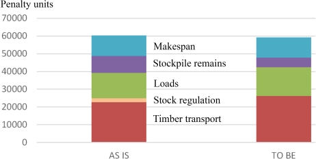
Figure 6.3. Performance indicators. For a color version of this figure, see www.iste.co.uk/bourrieres/networks.zip
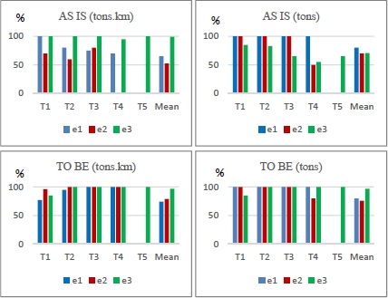
Figure 6.4. Load rate of transport resources. For a color version of this figure, see www.iste.co.uk/bourrieres/networks.zip
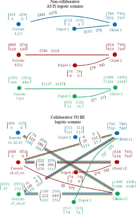
Figure 6.5. Material supply flows. For a color version of this figure, see www.iste.co.uk/bourrieres/networks.zip
- 1 After linearization of the “absolute value” operator appearing in the component of equation [6.4] of the objective function.