Herbrand Logic Proofs
7.1 INTRODUCTION
Logical entailment for Herbrand Logic is defined the same as for Propositional Logic. A set of premises logically entails a conclusion if and only if every truth assignment that satisfies the premises also satisfies the conclusions. In the case of Propositional Logic, we can check logical entailment by examining a truth table for the language. With finitely many proposition constants, the truth table is large but finite. For Herbrand Logic, things are not so easy. It is possible to have Herbrand bases of infinite size; and, in such cases, truth assignments are infinitely large and there are infinitely many of them, making it impossible to check logical entailment using truth tables.
All is not lost. As with Propositional Logic, we can establish logical entailment in Herbrand Logic by writing proofs. In fact, it is possible to show that, with a few simple restrictions, a set of premises logically entails a conclusions if and only if there is a finite proof of the conclusion from the premises, even when the Herbrand base is infinite. Moreover, it is possible to find such proofs in a finite time. That said, things are not perfect. If a set of sentences does not logically entail a conclusion, then the process of searching for a proof might go on forever. Moreover, if we remove the restrictions mentioned above, we lose the guarantee of finite proofs. Still, the relationship between logical entailment and finite provability, given those restrictions, is a very powerful result and has enormous practical benefits.
In this chapter, we start by extending the Fitch system from Propositional Logic to Herbrand Logic. We then illustrate the system with a few examples. Finally, we talk about soundness and completeness.
7.2 PROOFS
Formal proofs in Herbrand Logic are analogous to formal proofs in Propositional Logic. The major difference is that there are four additional mechanisms to deal quantified sentences.
The Fitch system for Herbrand Logic is an extension of the Fitch system for Propositional Logic. In addition to the ten logical rules of inference, there are four ordinary rules of inference for quantified sentences. Let’s look at each of these in turn. (If you’re like me, the prospect of going through a discussion of so many rules of inference sounds a little repetitive and boring. However, it is not so bad. Each of the rules has its own quirks and idiosyncrasies, its own personality. In fact, a couple of the rules suffer from a distinct excess of personality. If we are to use the rules correctly, we need to understand these idiosyncrasies.)
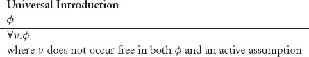
Universal Introduction (UI) allows us to reason from arbitrary sentences to universally quantified versions of those sentences.
Typically, UI is used on sentences with free variables to make their quantification explicit. For example, if we have the sentence hates(jane,y), then, we can infer ∀y.hates(jane,y).
Note that we can also apply the rule to sentences that do not contain the variable that is quantified in the conclusion. For example, from the sentence hates(jane,jill), we can infer ∀x.hates(jane,jill). And, from the sentence hates(jane,y), we can infer ∀x.hates(jane,y). These are not particularly sensible conclusions. However, the results are correct, and the deduction of such results is necessary to ensure that our proof system is complete.
There is one important restriction on the use of Universal Introduction. If the variable being quantified appears in the sentence being quantified, it must not appear free in any active assumption, i.e., an assumption in the current subproof or any superproof of that subproof. For example, if there is a subproof with assumption p(x) and from that we have managed to derive q(x)i, then we cannot just write ∀x.q(x).
If we want to quantify a sentence in this situation, we must first use Implication Introduction to discharge the assumption and then we can apply Universal Introduction. For example, in the case just described, we can first apply Implication Introduction to derive the result (p(x) ⇒ q(x)) in the parent of the subproof containing our assumption, and we can then apply Universal Introduction to derive ∀x.(p(x) ⇒ q(x)).
Universal Elimination (UE) allows us to reason from the general to the particular. It states that, whenever we believe a universally quantified sentence, we can infer a version of the target of that sentence in which the universally quantified variable is replaced by an appropriate term.

For example, consider the sentence ∀y.hates(jane,y). From this premise, we can infer that Jane hates Jill, i.e., hates(jane,jill). We also can infer that Jane hates her mother, i.e., hates(jane,mother(jane)). We can even infer than Jane hates herself, i.e., hates(jane,jane).
In addition, we can use Universal Elimination to create conclusions with free variables. For example, from ∀x.hates(jane,x), we can infer hates(jane,x) or, equivalently, hates(jane,y).
In using Universal Elimination, we have to be careful to avoid conflicts with other variables and quantifiers in the quantified sentence. This is the reason for the constraint on the replacement term. As an example of what can go wrong without this constraint, consider the sentence ∀x.∃y.hates(x, y), i.e., everybody hates somebody. From this sentence, it makes sense to infer ∃y.hates(jane,y), i.e., Jane hates somebody. However, we do not want to infer ∃y.hates(y, y); i.e., there is someone who hates herself.
We can avoid this problem by obeying the restriction on the Universal Elimination rule. We say that a term τ is substitutable for a variable ν in a sentence ϕ if and only if no free occurrence of ν occurs within the scope of a quantifier of some variable in τ Δ. For example, the term x is substitutable for y in ∃z.hates(y, z). However, the term z is not substitutable for y, since y is being replaced by z and y occurs within the scope of a quantifier of z. Thus, we cannot substitute z for y in this sentence, and we avoid the problem we have just described.
Existential Introduction (EI). If we believe a sentence ϕ[τ] that is the result of replacing every free occurrence of a variable ν by a term τ, then we can infer the existentially quantified sentence ∃ν.ϕ [ν].

The rule is stated in a way that requires thinking “backwards”. For example, from the sentence hates(jill,jill), we can infer that there is someone who hates herself, i.e., ∃x.hates(x,x), because hates(jill,jill) can be obtained from hates(x,x) by replacing every free occurrence of the variable x by the term jill. We can also infer that there is someone Jill hates, i.e., ∃x.hates(jill,x), because hates(jill,jill) can be obtained from hates(jill,x) by replacing every free occurrence of the variable x by the term jill. Finally, we can also infer that there is someone who hates Jill, i.e., ∃x.hates(x,jill), because hates(jill,jill) can be obtained from hates(x,jill) by replacing every free occurrence of the variable x by the term jill.
For a further example, by two applications of Existential Introduction, we can infer that someone hates someone, i.e., ∃x.∃y.hates(x,y).
Notice that the rule avoids certain unwarranted inferences. For example, starting from ∃x.hates(jane,x), one might be tempted to infer ∃x.∃x.hates(x,x). It is an odd sentence since it contains nested quantifiers of the same variable. Nevertheless, it is a legal sentence, and it states that there is someone who hates himself, which does not follow from the premise in this case.
The inference is disallowed under Existential Introduction because the premise ∃x.hates(jane,x), cannot be obtained from the sentence ∃x.hates(x,x) by replacing every free occurrence of x by jane.
Consider another example of a disallowed inference under Existential Introduction. If we disregarded the condition that τ be substitutable for ν in ϕ, we could start from the premise ∀x. ∃y.hates(x, y) (everyone hates someone) and infer the conclusion ∃z.∀x.∃y.hates(x, z) (there is a somebody whom everyone hates) because ∀x.∃y.hates(x, y) can be obtained from ∀x.∃y.hates(x, z) by replacing every free occurrence of z by y. The inference is disallowed under Existential Introduction because y is not substitutable for z in ∀x.∃y.hates(x, z).
Existential Elimination (EE). Suppose we have an existentially quantified sentence with target ϕ; and suppose we have a universally quantified implication in which the antecedent is the same as the scope of our existentially quantified sentence and the conclusion does not contain any free occurrences of the quantified variable. Then, we can use Existential Elimination to infer the consequent.

For example, if we have the sentence ∀x.(hates(jane,x) ⇒¬nice(jane)) and we have the sentence ∃x.hates(jane,x), then we can conclude ¬nice(jane).
It is interesting to note that Existential Elimination is analogous to Or Elimination. This parallel is expected because an existential sentence is effectively a disjunction. Recall that, in Or Elimination, we start with a disjunction with n disjuncts and n implications, one for each of the disjuncts and produce as conclusion the consequent shared by all of the implications. An existential sentence (like the first premise in any instance of Existential Elimination) is effectively a disjunction over the set of all ground terms; and a universal implication (like the second premise in any instance of Existential Elimination) is effectively a set of implications, one for each ground term in the language. The conclusion of Existential Elimination is the common consequent of these implications, just as in Or Elimination.
As in Chapter 3, we define a structured proof of a conclusion from a set of premises to be a sequence of (possibly nested) sentences terminating in an occurrence of the conclusion at the top level of the proof. Each step in the proof must be either (1) a premise (at the top level) or an assumption (other than at the top level) or (2) the result of applying an ordinary or structured rule of inference to earlier items in the sequence (subject to the constraints given above and in Chapter 3).
7.3 EXAMPLE
As an illustration of these concepts, consider the following problem. Suppose we believe that everybody loves somebody. And suppose we believe that everyone loves a lover. Our job is to prove that Jack loves Jill.
First, we need to formalize our premises. Everybody loves somebody. For all y, there exists a z such that loves(y,z).
∀y. ∃z.loves(y,z)
Everybody loves a lover. If a person is a lover, then everyone loves him. If a person loves another person, then everyone loves him. For all x and for all y and for all z, loves(y,z) implies loves(x,y).
∀x.∀y.∀z.(loves(y,z) ⇒ loves(x,y))
Our goal is to show that Jack loves Jill. In other words, starting with the preceding sentences, we want to derive the following sentence.
loves(jack,jill)
A proof of this result is shown below. Our premises appear on lines 1 and 2. The sentence on line 3 is the result of applying Universal Elimination to the sentence on line 1, substituting jill for y. The sentence on line 4 is the result of applying Universal Elimination to the sentence on line 2, substituting jack for x. The sentence on line 5 is the result of applying Universal Elimination to the sentence on line 4, substituting jill for y. Finally, we apply Existential Elimination to produce our conclusion on line 6.

Now, let’s consider a slightly more interesting version of this problem. We start with the same premises. However, our goal now is to prove the somewhat stronger result that everyone loves everyone. For all x and for all y, x loves y.
∀x.∀y.loves(x,y)
The proof shown below is analogous to the proof above. The only difference is that we have free variables in place of object constants at various points in the proof. Once again, our premises appear on lines 1 and 2. Once again, we use Universal Elimination to produce the result on line 3; but this time the result contains a free variable. Note that we have replaced the We get the results on lines 4 and 5 by successive application of Universal Elimination to the sentence on line 2. We deduce the result on line 6 using Existential Elimination. Finally, we use two applications of Universal Introduction to generalize our result and produce the desired conclusion.

This second example illustrates the power of free variables. We can manipulate them as though we are talking about specific individuals (though each one could be any object); and, when we are done, we can universalize them to derive universally quantified conclusions.
7.4 EXAMPLE
As another illustration of Herbrand Logic proofs, consider the following problem. We know that horses are faster than dogs and that there is a greyhound that is faster than every rabbit. We know that Harry is a horse and that Ralph is a rabbit. Our job is to derive the fact that Harry is faster than Ralph.
First, we need to formalize our premises. The relevant sentences follow. Note that we have added two facts about the world not stated explicitly in the problem: that greyhounds are dogs and that our faster than relationship is transitive.

Our goal is to show that Harry is faster than Ralph. In other words, starting with the preceding sentences, we want to derive the following sentence.
f (harry,ralph)
The derivation of this conclusion goes as shown below. The first six lines correspond to the premises just formalized. On line 7, we start a subproof with an assumption corresponding to the scope of the existential on line 2, with the idea of using Existential Elimination later on in the proof. Lines 8 and 9 come from And Elimination. Line 10 is the result of applying Universal Elimination to the sentence on line 9. On line 11, we use Implication Elimination to infer that y is faster than Ralph. Next, we instantiate the sentence about greyhounds and dogs and infer that y is a dog. Then, we instantiate the sentence about horses and dogs; we use And Introduction to form a conjunction matching the antecedent of this instantiated sentence; and we infer that Harry is faster than y. We then instantiate the transitivity sentence, again form the necessary conjunction, and infer the desired conclusion. Finally, we use Implication Introduction to discharge our subproof; we use Universal Introduction to universalize the results; and we use Existential Elimination to produce our desired conclusion.


This derivation is somewhat lengthy, but it is completely mechanical. Each conclusion follows from previous conclusions by a mechanical application of a rule of inference. On the other hand, in producing this derivation, we rejected numerous alternative inferences. Making these choices intelligently is one of the key problems in the process of inference.
7.5 EXAMPLE
In this section, we use our proof system to prove some basic results involving quantifiers.
Given ∀x.∀y.(p(x,y) ⇒ q(x)), we know that ∀x.(∃y.p(x,y) ⇒ q(x)). In general, given a universally quantified implication, it is okay to drop a universal quantifier of a variable outside the implication and apply an existential quantifier of that variable to the antecedent of the implication, provided that the variable does not occur in the consequent of the implication.
Our proof is shown below. As usual, we start with our premise. We start a subproof with an existential sentence as assumption. Then, we use Universal Elimination to strip away the outer quantifier from the premise. This allows us to derive q(x) using Existential Elimination. Finally, we create an implication with Implication Introduction, and we generalize using Universal Introduction.

The relationship holds the other way around as well. Given ∀x.(∃y.p(x,y) ⇒ q(x)), we know that ∀x.∀y.(p(x,y) ⇒ q(x)). We can convert an existential quantifier in the antecedent of an implication into a universal quantifier outside the implication.
Our proof is shown below. As usual, we start with our premise. We start a subproof by making an assumption. Then we turn the assumption into an existential sentence to match the antecedent of the premise. We use Universal Implication to strip away the quantifier in the premise to expose the implication. Then, we apply Implication Elimination to derive q(x). Finally, we create an implication with Implication Introduction, and we generalize using two applications of Universal Introduction.

RECAP
A Fitch system for Herbrand Logic can be obtained by extending the Fitch system for Propositional Logic with four additional rules to deal with quantifiers. The Universal Introduction rule allows us to reason from arbitrary sentences to universally quantified versions of those sentences. The Universal Elimination rule allows us to reason from a universally quantified sentence to a version of the target of that sentence in which the universally quantified variable is replaced by an appropriate term. The Existential Introduction rule allows us to reason from a sentence involving a term τ to an existentially quantified sentence in which one, some, or all occurrences of τ have been replaced by the existentially quantified variable. Finally, the Existential Elimination rule allows us to reason from an existentially quantified sentence ∃ν.φ[ν] and a universally quantified implication ∀ν.(φ[ν] ⇒ ψ) to the consequent ψ, under the condition that ν does not occur in ψ.