Chapter 10

Corporate Games III

Games Against the Competition

We now delve into the world of games between businesses. Of the myriad dimensions along which businesses can compete, we will discuss competition in choosing where to locate, pricing their products, by how many products they produce in the market, and by advertising.

10.1 Quantity Games: Everyone Can Win

One of the earliest, formal models that uses the logic of game theory was created by Antoine Augustin Cournot around 1838. Since Cournot was a mathematician, we will use a little bit of math in this section. He was observing two bottlers of spring water in a French town. He observed that the more spring water the two firms produced, the lower was the price that they could charge to sell their product following the well-known “law of demand”: the scarcer something is, the higher its price, and the more of a product there is, the lower the price must be in order to entice customers to buy all of it. Cournot constructed an equation that showed the relationship between quantity and price. Suppose the first bottler produced Q1 gallons on a certain day and the second bottler produced Q2 gallons, then the price might be given by an equation like:

Price = 10 – (Q1 + Q2)

For example, if both bottlers produced 4 gallons today, then they could sell their total of 8 gallons if they both charge a price of

Price = 10 – (4 + 4) = 10 – 8 = 2 francs

To keep this example as simple as possible, let’s assume that it costs these firms absolutely nothing to bottle the water. Then each firm has to choose how many gallons of water they are going to try to sell today in order to maximize how much revenue they get for selling it. In the previous ­example, each firm would receive two francs for each of four gallons of water for a total of 8 francs.

However, is this a reasonable outcome? If the first bottler saw the second bottler carrying 4 gallons to the town, how many gallons would he want to produce? The price function is now simplified a little bit:

Price = 10 – (Q1 + 4) = 10 – Q1 – 4 = 6 – Q1

The first bottler knows that the more he produces the lower the price will be that he will receive for his product. How many gallons should he ­produce in order to make the most money? Let’s look at the following table:

The first bottler’s best response when he sees the second bottler producing 4 gallons is to produce 3 gallons himself so that he ends up with revenue of 9 francs. Let’s do that one more time to make sure we understand the idea. Let’s suppose that Player 1 saw Player 2 produce 2 gallons today:

Price = 10 – (Q1 + 2) = 10 – Q1 – 2 = 8 – Q1.

Player 1’s best response to Player 2 producing 2 gallons must be 4 gallons! Cournot mathematically showed that there is an equation that describes Player 1’s best response. In this case, it looks like this:1

Best Quantity for Player 1 = 5 – ½ Q2

We call this equation the “best response function” for Player 1. Because in this simple example there is no difference between Player 1 and Player 2 in terms of the products they are selling or their costs, Player 2’s best response function is the same:

Best Quantity for Player 2 = 5 – ½ Q1

Now comes the core game theory question: how can we find a Nash equilibrium? Once again a let’s recall our definition of a Nash equilibrium:

Nash Equilibrium: A Nash Equilibrium is an outcome where neither player would want to change their decision after learning of the outcome. In other words, each player has made the best response to the other player’s choice.

So what we want to do is try to find quantities for each player where they have both made their best response to what the other has done. We could either solve these two equations for the two unknowns, or find the solution with a graph. In the subsequent figure, the Best Response lines for Players 1 and 2 are BR1 and BR2, respectively. Where they intersect, each has made a best response to the other’s amount produced, so it is a Nash equilibrium! On the graph we can see that this occurs at a little more than three units for each. The actual Nash equilibrium is where they both produce 3 units.

Let’s verify this using our Best Response Function for Player 1:

Best Quantity for Player 1 = 5 – ½ Q2 = 5 – ½ (3) = 5 – 1 = 3

The point to take away from all of this is that when players view the game from the standpoint of choosing the best response to the other player’s production level, both players end up making a profit. In this case, the price of each gallon of water will be 3 francs, and as each player also sells 3 gallons, each player will make a profit of 11.11 francs.

10.2 Pricing Games: We All Lose

About 45 years later another Frenchman named Joseph Louis François Bertrand observed firms competing by undercutting each other’s prices. So, rather than players reacting to the quantity that the other firm was producing, under cutthroat price competition all customers will buy their products from the lowest priced firm. What does a Nash equilibrium look like in this case?

Suppose that each firm was charging $2 per gallon of water, and they were selling 4 gallons each. Bertrand said that in this case one of the players would want to lower their price slightly, say to $1.99 per gallon. Because he is charging a lower price all customers would buy it from the player charging $1.99, and so this player would be selling all 8 gallons (actually, a little bit more since when the price goes down people want to buy a little more).

Now the player who was charging $2 is making no money at all! So, his best move is to charge $1.98. However, this is not an equilibrium either. Players will keep undercutting each other until they both cut their price to one penny above how much it costs them to produce each gallon of water (which we will assume was zero). So, the only equilibrium price in this game is for both to charge $.01 (assuming that one penny each is the lowest practical price possible).

In this kind of situation, firms are bringing in such a small amount of money that they will not have enough to cover their overheads, and will lose money and eventually go out of business. So, which model is “right”? Do firms react to each other by the quantity, or by the price? The surprising answer is that in industries where the amount of output is difficult to change, firms tend to react by changing output. However, if output is very easy to change, firms tend to react by using price competition. Why is this?

When output is difficult to change, firms are going to accept the ­highest price they can get for the output that they are capable of producing during that day. However, if they see that by investing more money to increase output would probably improve their profit, then they will do it. On the other hand, if it is easy for a firm to produce as much as it wants on any given day, then by lowering their price just a little bit lower than their competitor, they will have absolutely no problem filling the orders of everyone who comes to take advantage of their lower price. Sometimes we see price competition for short periods of time when there is “excess capacity” in a market, so firms have this ability to fill many more orders than they are currently getting. During the early 2000s, we saw oil tanker companies making high profits; at the time they were using quantity competition. Most of the world’s tanker firms estimated that they could increase their profits by increasing their capacities (building more tankers). However, by around 2010, tanker firms all had a lot of excess capacity, and price competition set in. By 2012 many tanker firms have gone bankrupt and tankers are now being sold for scrap metal.

10.3 Firm Location and Price

In 1929, Harold Hotelling wrote a paper called “Stability in Competition.” He observed many firms charging different prices for exactly the same product, and in contrast to what Bertrand said, all customers were not buying from the lower priced seller. Additionally, these prices were all higher than what it costs to produce the product, and these firms were not going out of business. The difference he found was that people don’t only go to the seller with the lowest price, they also take into consideration how far they have to travel in order to buy the product from each seller. Because time and distance traveled are costs just like money is, a person should not drive 10 miles just to save a penny on a product.

What Hotelling meant by “stability” is the fact that we do not see all customers switching back and forth between two different sellers as they change their price by a penny or two. Instead, what we might see is that a few customers who are located roughly in the middle between the two sellers might change their mind for a couple of pennies, but the large majority of customers will remain “stable,” continuing to shop where they always have.

So, even if one store is charging $8 and another is charging $10, the market might be divided like so (in the following figure), where the arrows tell us where customers live who will patronize each store, and the vertical line shows us the dividing line between patrons of each store. People are willing to drive from a longer distance away to get to the cheaper store.

However, if the store on the left were to cut their price to $6, the distribution of customers might look like this:

Of course, with a low enough price, one store could entice all of the customers to come to their store, but this would not be an equilibrium price, because the other store should lower their price enough to get some customers back. However, the incentive for cutthroat pricing is not very strong because cutting price only increases sales by a small amount.

The discussion so far illustrates how changing prices can affect sales for a store, given that their locations have already been decided. But how do these locations get decided in the first place?

10.4 Location Games: All Together, or Spread out?

One of the fundamental questions in retailing and in the restaurant industry is where to locate your business. On the one hand, you want to be close to your customers. On the other hand, you have to decide whether you should locate close to competing businesses or far away from them. Additionally, location can be a metaphor for how one chooses to “place” their product in the market, for example, a basic, midrange, or high-end product. In the breakfast cereal industry, a product might be placed along a continuum between “healthy” and “sugary fluff.”

In the real world, we certainly see both kinds of behaviors: We see that many businesses cluster together in malls or on Main Street (High Street, for the British), but we also see some types of stores that seem to avoid being near similar stores. In the United States, I have observed that clothing stores and restaurants tend to be of the clumpy variety—while grocery stores and gas stations are a little more likely to be of the solitary variety—it is uncommon to see two grocery stores located right next to each other. While it is somewhat common to see gas stations occur in pairs in a neighborhood, it is rare to see clusters of three or more, all in a row, as we do with restaurants or clothing stores.

The intuition here is fairly simple. Gas stations and grocery stores sell more or less identical products. So, it is not a great idea to locate too close to a competitor, because the closer you get the more likely you’ll end up competing only based on price, and end up losing money. If you’re far enough apart, you can take advantage of Hotelling’s “stability” which gives you some pricing flexibility.

Clothing stores and restaurants do not sell exactly the same thing. Because of this, the tendency to compete based on price is much smaller. It doesn’t make much sense to assume that people will say “the Chinese meal is $9.99 but the pizza is $10.00, so we are definitely all going to go eat Chinese.” And because every clothing store sells to a different kind of customer with different styles of clothing, these stores tend to cluster into clothes shopping districts. However, one would never imagine having a grocery store district or gas station district in a city.

10.5 The Purpose of Advertising

There are two main functions of advertising. The first is to increase the demand for a product, because the more you hear the name of a ­product the more likely you are to think about going and buying some of it. The second function of advertising is to try to differentiate your ­product from another very similar one. For example, without advertising, Pepsi Cola, Coca Cola, RC Cola, and Generic No-Name Cola would all appear to be identical substances: fizzy, sweet, high calorie beverages with caffeine.

If customers view all of these products is exactly the same, and they are all sold in the same place on the same aisle of the same grocery store for example, then we are back to the situation where price competition is likely to take over. Whoever spends the most money (assuming it is spent effectively) by having singers and sports stars making their products seem the coolest will be able to charge a premium price for their product, and will be less vulnerable to price cuts of competitors. Spending money on advertising “sets the product apart” from the competition just as a physical distance would, meaning that they will not lose all of their customers if they raise the price just a little bit.

10.6 A Basic Hotelling Location Game

Hotelling looked not only at prices that businesses can charge based on given locations, but also looked at the choice of locations. To focus the discussion only on location, let us assume that for some reason the prices that businesses are allowed to charge has been fixed at some level. ­Otherwise the analysis gets extremely tedious when you can both change your price and your location at the same time.

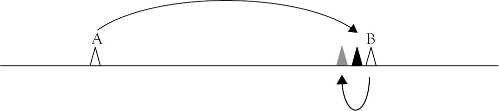
In this simple model, we assume that everyone lives evenly spread out along the same, one-mile-long street in a city. Everyone in the city wants to buy exactly 1 unit of your product from you, so the goal of the two business owners is to locate somewhere so that as many customers are closer to your store than the other store as possible in order to maximize your sales. In the simplest version of this game, we assume that the two stores have to plop down their stores somewhere simultaneously, and then we ask the age old question: are these locations a Nash equilibrium?

Look at the example locations in the following figure represented by the two hollow triangles, A and B. Are these a Nash equilibrium? Clearly, if we ask Store A if they would like to change their mind about where they located, it is clear that they would prefer to change their location. By moving their store just to the left side of the other store (to the Black Triangle location), they can greatly increase the number of customers that will find them to be the most convenient. However, this is not a Nash equilibrium either, because B could gain sales by moving just to the left of this new location for A. This “leapfrogging” would continue until both stores are located exactly at the middle. At this point, they both evenly split the market, and neither can gain any advantage by moving.

Political scientists have used this result as an analogy for “political positions” along the ideological spectrum. In the United States, where there are only two major political parties, the positions of the two parties are very similar in most ways, and both parties are fairly “centrist.”

In contrast, when there are three parties or three stores choosing to locate simultaneously, there is no set of locations under which at least one store does not regret their location and wants to change. If all three are located in the center, they each get one-third of the market. However, if one store moves slightly to the right or left, they can get almost one-half of the market, which is greater. In searching for an equilibrium from this point, an endless sequence of leapfrogging will occur. Again, this is used as a metaphor to explain the instability and often changing positions of parties in multiparty political systems around the world.

There are myriad other location games that have been analyzed by game theorists that are much more complicated that explore the interplay of location and pricing in different types of markets, and also to explain behavior by politicians in different political systems. As is true in the other parts of this brief book, we can only scratch the surface here.