The Basics—Multiple-Channel, Single-Phase Model
When the demand exceeds the output of a business, either that business must become more productive, increasing its output rate to cope with the increased demand, or adding more capacity to satisfy it. In a service situation, you either reduce your average service time per server or you add more servers. In this chapter, we will expand the waiting line analysis to take into account the effects of adding more servers. In chapter 6, we will explore the alternative of reducing service time.
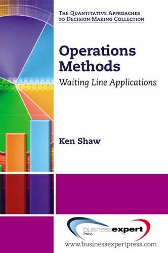
Figure 3.1 shows a simple multiple-channel, single-phase model M/M/s with two servers. Two queue configurations are possible: a separate line for each server and one queue feeding both servers.
Grocery and retail store checkout lines, traffic lanes, and old-style ticket counters are common examples of the separate lines configuration, and most banks and post offices are common examples of the single line configuration1 that directs each customer to the next available server. Some authors refer to the single line arrangement as a “snake” configuration because it often requires a winding layout to accommodate its length. A common example is the arrangement at airports before the passenger security checkpoints.
You may think that analyzing this will be easy. All you would have to do is either multiply the service rate by the number of servers for a single line feeding two servers or divide the arrival rate in half for two separate lines and then use the performance measures discussed in chapter 2 for the single-channel, single-phase model M/M/1. However, this is incorrect for a single service location with more than one server because the number of customers for one server is not independent of the number of customers for the other server. There are other nuances to be considered, such as the probability of no customers for one server when the other server is still busy, the probability that a newly arriving customer will pick a particular line in the separate line per server configuration, or the probability that a customer in a slowly moving line will change lines to a more quickly moving line (a process called jockeying).

Figure 3.1. Multiple-server waiting line configurations: (a) separate line per server and (b) one line feeding both servers.
To analyze the basic behavior of this model, we must make some assumptions, where the full Kendall notation for the model is M/M/s/∞/∞/FCFS:
- The arrival rate distribution is described by a Poisson distribution using an average rate λ, which means that the interarrival times can be characterized by an exponential distribution with an average interarrival time of 1/λ. Interarrival times are independent of the number of customers in the system.
- The service time distribution for each server is defined by an exponential distribution with an average service time of 1/µ, where µ represents the average service rate. The service rates are the same2 for each server. Obviously, a new server is likely to not be as productive as an experienced server. However, keep in mind that the waiting line equations are based on a steady-state condition, which implies that the new server has attained the average service rate capability. How long this may take is discussed in more detail in chapter 5.
- Service times are independent of the number of customers in the system.
- The number of phases in the service is one. We are assuming here that each server can do everything for the customer in the respective business: take the customer’s request, perform the necessary actions, and collect any payment. However, in many businesses where there is a higher volume of customers and several employees, some of these actions are likely to be assigned to only one or more of the servers. We will discuss some of these complexities in chapter 5.
- The arrival or calling population is infinite in size. This avoids complications introduced by the possibility of having served all available customers.
- The length of the waiting line(s) can be infinite. Although not really possible in real-world situations, this avoids analysis complications introduced by the rare possibility that some customers are blocked from entering the line. We will discuss the effects of limited line lengths in later chapters.
- The priority rule is first come, first served (FCFS).
- Balking or reneging by customers is not considered in the analysis.
- Jockeying is allowed in separate line configurations.
- The average arrival rate is less than the average total service rate (λ < sµ). That is, the multichannel utilization factor (ρs = λ/sµ) is less than 1.
This last requirement clarifies an error that occasionally occurs: Some texts consistently use a value for ρ as defined for the M/M/1 model in their equations for the M/M/s model, while other texts use a ρ value equivalent to ρs but without the s subscript to indicate that their use of ρ has a different definition in the M/M/s equations. In this monograph, ρ always represents λ/µ, and ρs is used to represent λ/sµ. Thus, ρs = ρ/s. For a given average arrival rate and an average service rate per server, the minimum number of servers must then be greater than λ/µ. The actual number of servers for many situations is likely to be greater than this minimum number to achieve desired performance values.
As for the M/M/1 model discussed in chapter 2, there are different versions of some of the performance measure equations in the literature regarding queuing analysis. Some alternate versions are provided here for your reference, with what I consider to be the more common version listed first. The various performance measures are listed in the same order as they are presented for the M/M/1 model in chapter 2. Additional measures special to the M/M/s model are discussed in chapter 5. You are reminded that the term system includes not only the number of customers waiting in line but also the customer(s) being served.
- M/M/s utilization factor: ρs = λ/sµ: for an M/M/s model, this value must be less than 1 for the following equations to be valid.
- Probability of zero customers in the system: The equation for P0 here is more complicated:3
 (3.1)
(3.1) - Probability of exactly n customers in the system: This equation has different forms dependent on n compared to the number of servers:
 (3.2)
(3.2) - Probability that the number of customers in the system is equal to or greater than the number of servers (e.g., all the operators in a call center are busy):
 (3.3)
(3.3) - The average number of customers in the system:

or, alternatively,
 (3.4)
(3.4) - The average total time customers spend in the system:
W = L/λ = (Lq/λ) + (1/µ).
- The average number of customers waiting in the queue (not yet being served):
Lq = L – (λ/µ),
or, alternatively,
 (3.5)
(3.5) - The average time customers wait in the queue before being served:
Wq = Lq/λ.
Now, let us examine these expressions. First, we consider the case where s = 1. This is the M/M/1 model. Do the equations reduce down to the equations given in chapter 2 for the M/M/1 model? Because they should, this is a good check for both typographical errors when using the multiple-channel equations from your favorite reference and for validating your understanding of what the more advanced mathematical notation signifies.
My classroom experiences indicate that it would be useful to review some mathematical notation to save you the time of looking it up for yourself.
The exclamation point indicates a factorial expression, where
n! = 1 × 2 × . . . × (n – 1) × n.
when n = 0, n! = 1. Any value raised to a power of zero is 1. For example, (x – 1)0 = 1.
The summation term ![]() is shorthand notation for x0 + x1 + x2 + . . . +
is shorthand notation for x0 + x1 + x2 + . . . +
xn+1 + xn, where i is a counter that represents the parameter range from 0 to n. Of course, x0 = 1.
Returning now to the equations at hand, the key parameter that must be derived first is P0 because its value is necessary to determine the other measures. Equation 3.1 can be a nasty piece of work with increasing chances of making a mathematical error when there are many servers to deal with. Likewise, determining L (Equation 3.4) also requires care. The equations for L and P0 can be expressed differently using only the value for s and the ratio of λ/µ. This allows an easier computation and enables the creation of reference tables for P0, Lq, and L for various combinations of λ/µ and s when using the M/M/s model. These tables are provided in appendix C.
The good news is that the expressions for queue length and waiting times are quite simple thanks to Little’s Law.
The probability of just n customers in the system (Equation 3.2) is useful for determining how likely it is that one or more servers are idle. This helps later when scheduling workloads in a place like a grocery store because it gives you an estimate of the slack time available for servers, who may then, for example, help to restock shelves.
Another useful observation is that a service manager can obtain an estimate of the overall average waiting time per customer by merely tallying the number of customers who enter the business during some selected time interval and counting the number of customers in the business at the end of that time interval. By collecting this information for several selected time periods, say every 15 minutes during a typical business day, you can average the results to obtain estimates of L and λ. Hence, using Little’s Law, W = L/λ. An example of this will be discussed in chapter 7.
Example 3.1. Coffee Shop With Two Servers
Let’s return to the Ken’s Caffeine Fix example in chapter 2. The coffee shop has an average arrival rate (λ) of 24 customers per hour and an average service rate (µ) of 1 customer every 2 minutes = 30 customers/hour. Recall that the average time spent waiting to be served in that coffee shop was 8 minutes, which is much too long for the typical office worker desiring a cup of coffee on his or her break. The average line length was 3.2 customers.
One solution to reduce the waiting time is for the owner to hire another server to increase the overall service rate for the coffee shop. So, plugging in the values for two servers in Equation 3.1 for P0, we should get

You may ask, “Is this value correct? We only doubled the number of servers, but P0 has more than doubled compared to the M/M/1 model.” The answer is yes, and it indicates that simply doubling the service rate of a single server is not the same as adding another server. This observation has important implications when deciding whether to hire another person or invest in service improvements (chapter 6). Table 3.1 compares the performance measure results for the M/M/1, M/M/2, M/M/1 with µ doubled, and M/M/1 with λ halved approaches. This will help illustrate why such simplified approaches, although they look like they would intuitively work, do not provide accurate answers.
Some readers may also ask, “Why are the answers expressed in so many significant digits?” In queuing analysis, particularly for the more complex models, it is important that you maintain as much precision as possible in the intermediate computations until you obtain the final result, which then can be rounded to a less detailed answer. Not doing this can have a noticeable effect on the final result. Not being aware of this creates considerable confusion for students who are doing homework together because when they compare their results, their answers often do not agree—leading them to assume that one of them has made a mistake.
Now that we have the value for P0, we can determine the probability that just one server will be idle. Using Equation 3.2 for one server idle (i.e., n = 1 customer in the system), this is simply
λP0/µ = ρP0 = 0.343.
Again, this is useful to know when considering how much of a new employee’s time can be used for work not directly related to serving customers.
Determining the probability of more than 5 customers in the shop is much more complicated than the simple formula used for the M/M/1 model. Now we need to determine the respective probabilities of just 0, 1, 2, 3, 4, and 5 customers in the shop using Equation 3.2, add those values together, and then, recalling that the total of all possible probabilities must equal 1, subtract that sum from 1 to obtain the probability we seek. Without showing the intermediate calculations, the values in this example are P1 = 0.343, P2 = 0.137, P3 = 0.055, P4 = 0.022, and P5 = 0.009. This gives a value for Pn>5 = 0.006 or 0.6%, which is a large improvement over the 26.2% value for the M/M/1 model.
Now we consider our major concern, “How much did we reduce the average waiting time?” First, we need to calculate the average line length using Equation 3.4. Plugging in the numbers using the P0 value determined earlier, we should get

Dividing L by λ gives us a total average waiting time of 0.039682 hour, or roughly 2.4 minutes, which is a much more reasonable time to get a cup of coffee. The corresponding average length of the queue is now 0.152381 customer, and the average wait in line is less than a minute at 22.9 seconds.
| Table 3.1. Comparison of the Results Using Correct Analysis Methods With the Results Using Incorrect Methods (Shaded Results) | ||||
|---|---|---|---|---|
| M/M/1 | M/M/2 | M/M/1 (2µ) | M/M/1 (λ/2) | |
| P0 | 0.2 | 0.428 | 0.600 | 0.600 |
| L | 4 | 0.952 | 0.667 | 0.667 |
| Lq | 3.2 | 0.152 | 0.267 | 0.267 |
| W | 10 minutes | 2.38 minutes | 3.33 minutes | 1.67 minutes |
| Wq | 8 minutes | 0.38 minute | 1.33 minutes | 0.67 minute |
Finally, let’s return to the earlier comment about why one should not use the M/M/1 equations in chapter 2 for determining the enhanced performance provided by adding another server. Referring to Table 3.1, if one doubles the service rate using a single line, the average line appears to be shorter than the M/M/2 solution, but the average total wait is longer. If one assumes that customers will evenly split between separate lines for each server (i.e., halving the arrival rate), the average line length and the average total waiting time are both smaller than for the M/M/2 solution. What are the reasons for not being able to use the results in the shaded cells of Table 3.1?
As will be explored further in subsequent chapters, there are several subtle things going on here. One server working at an average of 30 seconds per customer is not the same as the combination of two servers each working at an average of 1 minute per customer. The average throughput is the same, but the combined variance in the service rate for two servers is not the same as the variance for a single server. In addition, the average service rate of 2µ is valid only when both servers are busy. When only one server is busy, the service rate is µ.
Referring to our discussion of state diagrams in chapter 1, let us change the situation from a single-channel system to a multiple-channel system with two servers. An example would be a call center with two operators and no ability to have callers on hold. The output from state 2 back to state 1 shown in Figure 1.3 would be 2µ for a two-server system. The set of expressions for Equation 1.3 would change to
State 0: (P1 × µ) = (P0 × λ),
State 1: (P0 × λ) + (P2 × 2µ) = (P1 × λ) + (P1 × µ),
State 2: (P1 × λ) = (P2 × 2µ).
Solving for P0, P1, and P2 in the same manner as described in chapter 1, we obtain
P0 = 1/[1 + ρ + (ρ2/2)],
P1 = ρ/[1 + ρ + (ρ2/2)],
P2 = (ρ2/2)/[1 + ρ + (ρ2/2)].
The results show a relative increase in the probabilities of states 0 and 1 and a corresponding decrease in the probability of state 2, as we should expect. Again, adding P0, P1, and P2, we obtain a value of 1 as a check on our derivation.
When a customer enters a shop with two lines, the customer normally picks the shorter line, but he or she can pick the longer line if the customer perceives that the shorter line has a customer ahead in line that is likely to require a much longer service time (e.g., a person with a large number of packages at the post office).
Customers may change lines if the line they are in is moving slower than the other line. (We all have done this in slow-moving traffic when given an opportunity to move into a faster moving lane.) This behavior is called jockeying. The configuration of a single line feeding the next available server prevents jockeying and reduces the chances that a new customer will get stuck in a line behind a customer requiring a long service time.
You can divide the arrival rate if you add another server at a separate location so that the possibility of customers choosing or jockeying between the lines is eliminated. Then the two lines can be considered to be independent of each other, and each can be analyzed separately using the M/M/1 model equations. In such situations, the arrival rate for each location is determined by dividing the original total arrival rate according to what percentage you estimate will go to each location.
You can have an average total waiting time that is less than the average service time when the customer volume is low (ρ < 0.5) because the probability of a long service time delaying other customers is reduced. In effect, you are averaging the service time at one window with a customer with zero service time at the windows with no customers. In addition, when you use an exponential distribution to describe the range of possible service times, there is a cumulative probability that at least 63% of the possible service times will be shorter than the average service time. Correspondingly, the cumulative probability for possible service times greater than the average service time is therefore 37%. If the service time can be more accurately represented with a normal distribution, such as businesses providing only standardized services, these cumulative probabilities would each be 50%.