Once we create DataFrames, we can perform many operations on them. Some operations will reshape a DataFrame to add more features to it or remove unwanted data. Operations on DataFrames are also helpful in getting insights of the data using exploratory analysis.
This chapter discusses DataFrame filtering, data transformation, column deletion, and many related operations on a PySpark SQL DataFrame.
We cover the following recipes. Each recipe is useful and interesting in its own way. I suggest you go through each one once.
Recipe 4-1. Transform values in a column of a DataFrame
Recipe 4-2. Select columns from a DataFrame
Recipe 4-3. Filter rows from a DataFrame
Recipe 4-4. Delete a column from an existing DataFrame
Recipe 4-5. Create and use a PySpark SQL UDF
Recipe 4-6. Label data
Recipe 4-7. Perform descriptive statistics on a column of a DataFrame
Recipe 4-8. Calculate covariance
Recipe 4-9. Calculate correlation
Recipe 4-10. Describe a DataFrame
Recipe 4-11. Sort data in a DataFrame
Recipe 4-12. Sort data partition-wise
Recipe 4-13. Remove duplicate records from a DataFrame
Recipe 4-14. Sample records
Recipe 4-15. Find frequent items
Note
My intention behind repeating some lines of code is to provide less distraction while you are going through the step-by-step solution of a problem. Missing code lines force readers to go to previous chapters or to previous pages to make connections. When all the code chunks are together, the flow is clear and logical and it’s easier to understand the solution.
Recipe 4-1. Transform Values in a Column of a DataFrame
Problem
You want to apply a transformation operation on a column in a DataFrame.
Solution
There is a swimming competition. The length of the swimming pool is 20 meters. The number of participants in the competition is 12. The swim time in seconds has been noted. Table 4-1 depicts the details of the participants.
Table 4-1
Sample Data for the Swimming Competition
id
Gender
Occupation
swimTimeInSecond
id1
Male
Programmer
16.73
id2
Female
Manager
15.56
id3
Male
Manager
15.15
id4
Male
RiskAnalyst
15.27
id5
Male
Programmer
15.65
id6
Male
RiskAnalyst
15.74
id7
Female
Programmer
16.8
id8
Male
Manager
17.11
id9
Female
Programmer
16.83
id10
Female
RiskAnalyst
16.34
id11
Male
Programmer
15.96
id12
Female
RiskAnalyst
15.9
The assignment is to, using the data in Table 4-1, calculate the swimming speed for each swimmer and add it as a new column to the DataFrame, as shown in Table 4-2.
Table 4-2
Swimming Speed Column Added
id
Gender
Occupation
swimTimeInSecond
swimmerSpeed
id1
Male
Programmer
16.73
1.195
id2
Female
Manager
15.56
1.285
id3
Male
Manager
15.15
1.32
id4
Male
RiskAnalyst
15.27
1.31
id5
Male
Programmer
15.65
1.278
id6
Male
RiskAnalyst
15.74
1.271
id7
Female
Programmer
16.8
1.19
id8
Male
Manager
17.11
1.169
id9
Female
Programmer
16.83
1.188
id10
Female
RiskAnalyst
16.34
1.224
id11
Male
Programmer
15.96
1.253
id12
Female
RiskAnalyst
15.9
1.258
If we want to do an operation on each element of a column in the DataFrame, we have to use the withColumn() function.
The withColumn() function is defined on the DataFrame object. This function can add a new column to the existing DataFrame or it can replace a column with a new column containing new data. We have to use some expression to get the data of the new column.
How It Works
Step 4-1-1. Creating a DataFrame
The first step is the simplest one. As we discovered in the previous chapter, we can read a CSV file and create a DataFrame from it.
In [1]: swimmerDf = spark.read.csv('swimmerData.csv',
header=True, inferSchema=True)
In [2]: swimmerDf.show(4)
+----+------+-----------+----------------+
| id|Gender| Occupation|swimTimeInSecond|
+----+------+-----------+----------------+
| id1| Male| Programmer| 16.73|
| id2|Female| Manager| 15.56|
| id3| Male| Manager| 15.15|
| id4| Male|RiskAnalyst| 15.27|
+----+------+-----------+----------------+
only showing top 4 rows
The swimmerDf DataFrame has been created. We used the inferSchema argument set to True. It means that PySpark SQL will infer the schema on its own. Therefore, it is better to check it. So let’s print it using the printSchema() function.
In [3]: swimmerDf.printSchema()
Here is the output:
root
|-- id: string (nullable = true)
|-- Gender: string (nullable = true)
|-- Occupation: string (nullable = true)
|-- swimTimeInSecond: double (nullable = true)
Step 4-1-2. Calculating Swimmer Speed for Each Swimmer and Adding It as a Column
How do we calculate the swimmer speed? Speed is defined as distance over time, which we can calculate using the withColumn() function as an expression. We have to calculate the speed of each swimmer and add the results as a new column. The following line of code serves this purpose.
In [4]: swimmerDf1 = swimmerDf.withColumn('swimmerSpeed',20.0/swimmerDf.swimTimeInSecond)
We know that the withColumn() function returns a new DataFrame. The new column will be added to the newly created DataFrame called swimmerDf1. We can verify this using the show() function.
In the swimmerDf1 DataFrame, we can see that swimmerSpeed is the last column. If we want to round the values in the swimmerSpeed column, we can use the round() function, which is in the pyspark.sql.functions submodule. To work with it, we have to import it. The following code line imports the round() function from the pyspark.sql.functions submodule.
In [6]: from pyspark.sql.functions import round
Step 4-1-3. Rounding the Values of the swimmerSpeed Column
The round() function can be used with the withColumn() function. We are going to use the col argument of the withColumn() function. The first argument of the round() function is the swimmerSpeed column and the second argument is scale. The scale argument defines the format of a decimal number, which is how many digits we need after the decimal point. We are setting the scale to 3.
In [7]: swimmerDf2 = swimmerDf1.withColumn('swimmerSpeed', round(swimmerDf1.swimmerSpeed, 3))
You want to select one or more columns from a DataFrame.
Solution
We are going to use the swimmerDf2 DataFrame that we created in Recipe 4-1. Table 4-3 shows this DataFrame.
Table 4-3
The Dataframe
id
Gender
Occupation
swimTimeInSecond
swimmerSpeed
id1
Male
Programmer
16.73
1.195
id2
Female
Manager
15.56
1.285
id3
Male
Manager
15.15
1.32
id4
Male
RiskAnalyst
15.27
1.31
id5
Male
Programmer
15.65
1.278
id6
Male
RiskAnalyst
15.74
1.271
id7
Female
Programmer
16.8
1.19
id8
Male
Manager
17.11
1.169
id9
Female
Programmer
16.83
1.188
id10
Female
RiskAnalyst
16.34
1.224
id11
Male
Programmer
15.96
1.253
id12
Female
RiskAnalyst
15.9
1.258
We have to perform the following:
Select the swimTimeInSecond column.
Select the id and swimmerSpeed columns.
Which DataFrame API is going to help us? Here, the select() function will be working for us. This select() function is similar to the SELECT clause in SQL.
The select() function is defined in the DataFrame class. An argument of the select() function is columns, which we might want to select.
How It Works
Step 4-2-1. Selecting the swimTimeInSecond Column
The select() function can take a variable number of arguments. Its variable number of arguments will be the different columns we want to select. Let’s select the swimTimeInSecond column.
In [1]: swimmerDf3 = swimmerDf2.select("swimTimeInSecond")
In [2]: swimmerDf3.show(6)
Here is the output:
+----------------+
|swimTimeInSecond|
+----------------+
| 16.73|
| 15.56|
| 15.15|
| 15.27|
| 15.65|
| 15.74|
+----------------+
only showing top 6 rows
The output is shown in the swimmerDf3 DataFrame.
Step 4-2-2. Selecting the id and swimmerSpeed Columns
Now it is time to select the id and swimmerSpeed columns. The following line of code will perform the same.
In [3]: swimmerDf4 = swimmerDf2.select("id","swimmerSpeed")
In [4]: swimmerDf4.show(6)
Here is the output:
+---+------------+
| id|swimmerSpeed|
+---+------------+
|id1| 1.195|
|id2| 1.285|
|id3| 1.32|
|id4| 1.31|
|id5| 1.278|
|id6| 1.271|
+---+------------+
only showing top 6 rows
The swimmerDf4 DataFrame shows our required result.
The select() function takes an expression on the column. What is an expression in the context of programming? An expression is a statement that results in either a mathematical or logical value. In the following code line, we are going to select columns such that in the new DataFrame called swimmerDf5, the first column will be id and the second column will be the swimmerSpeed multiplied by 2.
In [5]: swimmerDf5 = swimmerDf2.select("id",swimmerDf2.swimmerSpeed*2)
In the previous code line, swimmerDf2.swimmerSpeed*2 is an expression.
In [6]: swimmerDf5.show(6)
Here is the output:
+---+------------------+
| id|(swimmerSpeed * 2)|
+---+------------------+
|id1| 2.39|
|id2| 2.57|
|id3| 2.64|
|id4| 2.62|
|id5| 2.556|
|id6| 2.542|
+---+------------------+
only showing top 6 rows
The final output is on display.
Recipe 4-3. Filter Rows from a DataFrame
Problem
You want to apply filtering to a DataFrame.
Solution
The filtering process is used to remove unwanted data from a dataset. It is the process of getting a required data subset from a dataset based on some condition. Datasets often come with unwanted records, therefore filtering is inevitable.
We are going to use the swimmerDf2 DataFrame and solve the following:
Select records where the Gender column has a value of Male.
Select records where Gender is Male and Occupation is Programmer.
Select records where Occupation is Programmer and swimmerSpeed > 1.17.
We are going to use the filter() function. This function filters records using a given condition. We provide the filtering condition as an argument to the filter() function. It returns a new DataFrame. The where() function is an alias of the filter() function. If two functions are aliases of each other, we can use them interchangeably with the same argument and get the same result.
How It Works
Step 4-3-1. Selecting Records Where the Gender Column Is Male
The argument of the filter function is a condition to show equality. We can show equality using swimmerDf2.Gender == 'Male'.
In [1]: swimmerDf3 = swimmerDf2.filter(swimmerDf2.Gender == 'Male')
Step 4-3-2. Selecting Records Where Gender Is Male and Occupation Is Programmer
We can provide compound logical expressions in the filter() function. But core Python and and or operators will not work. We have to provide the & operator for and and use the | operator for or.
Recipe 4-4. Delete a Column from an Existing DataFrame
Problem
You want to delete some columns from a DataFrame.
Solution
Data scientists can get structured datasets in which some columns are redundant and must be removed before analysis.
In this recipe, you want to accomplish the following:
Drop the id column from the swimmerDf2 DataFrame.
Drop the id and Occupation columns from swimmerDf2.
The drop() function can be used to drop one or more columns from a DataFrame. It takes columns to be dropped as its argument. It returns a new DataFrame. The new DataFrame will not contain the dropped columns.
How It Works
Step 4-4-1. Dropping the id Column from the swimmerDf2 DataFrame
We start by dropping the id column:
In [1]: swimmerDf3 = swimmerDf2.drop(swimmerDf2.id)
Step 4-4-2. Dropping the id and Occupation Columns from swimmerDf2
Deleting or dropping more than one column is very easy. We have to provide all the columns as strings and the number of arguments as variables to the drop() function:
In [5]: swimmerDf5 = swimmerDf2.drop("id", "Occupation")
In [6]: swimmerDf5.show(6)
Here is the output:
+------+----------------+------------+
|Gender|swimTimeInSecond|swimmerSpeed|
+------+----------------+------------+
| Male| 16.73| 1.195|
|Female| 15.56| 1.285|
| Male| 15.15| 1.320|
| Male| 15.27| 1.310|
| Male| 15.65| 1.278|
| Male| 15.74| 1.271|
+------+----------------+------------+
only showing top 6 rows
We have our final result in the swimmerDf5 DataFrame.
Recipe 4-5. Create and Use a PySpark SQL UDF
Problem
You want to create a user-defined function (UDF) and apply it to a DataFrame column.
Solution
You might be thinking that everyone who knows Python can create a user-defined function easily. What is so special about them? But, here in PySpark SQL, UDFs work on a column. A UDF works on each element of a column, which results in a new column.
Figure 4-1 shows the average temperature collected in Celsius over seven days and how we can add a column that translates the temperatures to degrees Fahrenheit.
Figure 4-1
Adding a Fahrenheit column
As we can see in Figure 4-1, the table on the left has day as the first column and temperature in Celsius as the second column. For us, this table is a DataFrame. We have to create a new DataFrame, which is shown on the right side of Figure 4-1. This new DataFrame has a third column, which lists the temperature in Fahrenheit. For each value in column two, we are transforming that value into degrees Fahrenheit in column three.
It seems a very simple problem. We first create a Python function that will take a temperature value in Celsius and return that temperature in Fahrenheit. You might wonder if there is an existing function to perform this task. How do we apply the created function to each value in the column? Are we going to use some sort of loop? No, we just have to make this function a UDF and the rest will be taken care by the PySpark SQL API’s function withColumn().
Transforming a simple Python function into a UDF is very simple. We are going to use the udf() function, as follows:
udf(f= None, returnType =StringType)
The udf() function is defined in the PySpark submodule pyspark.sql.functions. It takes two arguments. The first argument is a Python function and the second argument is the return datatype of this function. The return datatype will be from the PySpark submodule pyspark.sql.types. The default value of the returnType argument is StringType.
We are going to solve the given problem in a step-by-step fashion.
How It Works
Step 4-5-1. Creating a DataFrame
We have been given data in a Parquet file. The name of the data directory is temperatureData. We need the DoubleType class and the udf function. Therefore, first we are going to import the required function and class.
In [1]: from pyspark.sql.types import DoubleType
from pyspark.sql.functions import udf
From Spark 2.0.0 and onward, it is very easy to read data from different sources, which we have discussed in detail in previous chapters. In order to read data from a Parquet file, we have to use the spark.read.parquet() function, where the spark is an object of the SparkSession class. This spark object is provided by the console.
In [2]: tempDf = spark.read.parquet('temperatureData')
In [3]: tempDf.show(6)
Here is the output:
+----+-------------+
| day|tempInCelsius|
+----+-------------+
|day1| 12.2|
|day2| 13.1|
|day3| 12.9|
|day4| 11.9|
|day5| 14.0|
|day6| 13.9|
+----+-------------+
only showing top 6 rows
Step 4-5-2. Creating a UDF
Creating a PySpark SQL UDF is in general a two-step process. First we have to create a Python function for the purpose and then we have to transform the created Python function to a UDF function using the udf() function.
To transform the Celsius values into Fahrenheit, we create a Python function called celsiustoFahrenheit. This function has one argument called temp, which is temperature in Celsius.
In [4]: def celsiustoFahrenheit(temp):
...: return ((temp*9.0/5.0)+32)
...:
Let’s test the working of our Python function.
In [5]: celsiustoFahrenheit(12.2)
Out[5]: 53.96
The test result shows that the celsiustoFahrenheit function is working as expected. Now let’s transform our Python function to a UDF.
In [6]: celsiustoFahrenheitUdf = udf("celsiustoFahrenheit", DoubleType())
We can observe that the udf() function has taken the name of the function in String format as its first argument and the return type of the UDF as the second argument. The return type of our UDF is DoubleType. Here, celsiustoFahrenheitUdf is our required UDF. It will be applied to each value in the tempInCelsius column and return the temperature in degrees Fahrenheit.
Step 4-5-3. Using the UDF to Create a New Column
The required UDF has been created. So, we’ll now use this UDF to transform the temperature from Celsius to Fahrenheit and add the result as a new column. We are going to use the withColumn() function with a second argument as a UDF and with tempInCelsius as the input to the UDF.
In [7]: tempDfFahrenheit = tempDf.withColumn('tempInFahrenheit', celsiustoFahrenheitUdf(tempDf.tempInCelsius))
In [7]: tempDfFahrenheit.show(6)
Here is the output:
+----+-------------+----------------+
| day|tempInCelsius|tempInFahrenheit|
+----+-------------+----------------+
|day1| 12.2| 53.96|
|day2| 13.1| 55.58|
|day3| 12.9| 55.22|
|day4| 11.9| 53.42|
|day5| 14.0| 57.20|
|day6| 13.9| 57.02|
+----+-------------+----------------+
only showing top 6 rows
The tempDfFahrenheit output shows that we have completed the recipe successfully.
Step 4-5-4. Saving the Resultant DataFrame as a CSV File
It’s a good idea to save the results for further use.
In [8]: tempDfFahrenheit.write.csv(path='tempInCelsAndFahren',header=True,sep=',')
The result is in the part-00000-1320146a-7998-4f3b-9bdd-939227c793c9-c000.csv file.
Recipe 4-6. Data Labeling
Problem
You want to label the data points in a DataFrame column.
Solution
We have dealt with temperature data in Recipe 4-5. See Figure 4-2.
Figure 4-2
Labeling the data
Figure 4-2 displays our job for this recipe. We have to label the data in the tempInCelsius column. We have to create a new column named label. This label will report High if the corresponding tempInCelsius value is greater than 12.9 and Low otherwise.
How It Works
Step 4-6-1. Creating the UDF to Create a Label
We know that we need a udf() function because we have to create a UDF that can create labels.
In [1]: from pyspark.sql.functions import udf
We are going to create a Python function named labelTemprature. This function will take the temperature in Celsius as the input and return High or Low, depending on the conditions.
In [2]: def labelTemprature(temp) :
...: if temp > 12.9 :
...: return "High"
...: else :
...: return "Low"
In [3]: labelTemprature(11.99)
Out[3]: 'Low'
In [4]: labelTemprature(13.2)
Out[4]: 'High'
Let’s create a PySpark SQL UDF using labelTemprature.
In [5]: labelTempratureUdf = udf(labelTemprature)
Step 4-6-2. Creating a New DataFrame with a New Label Column
The new DataFrame called tempDf2 is created with a new column label using the withColumn() function:
In [6]: tempDf2 = tempDf.withColumn("label", labelTempratureUdf(tempDf.tempInCelsius))
In [7]: tempDf2.show()
Here is the output:
+----+-------------+-----+
| day|tempInCelsius|label|
+----+-------------+-----+
|day1| 12.2| Low|
|day2| 13.1| High|
|day3| 12.9| Low|
|day4| 11.9| Low|
|day5| 14.0| High|
|day6| 13.9| High|
|day7| 12.7| Low|
+----+-------------+-----+
We have labeled the data.
Recipe 4-7. Perform Descriptive Statistics on a Column of a DataFrame
Problem
You want to calculate descriptive statistics measures on columns in a DataFrame.
Solution
Descriptive statistics provide you with important information about your data. The important descriptive statistics are count, sum, mean, sample variance, and sample standard deviation. Let’s discuss them one by one.
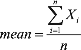
Consider the data points x1, x2, . . ,xn from the variable x. Figure 4-3 shows the mathematical formula for how to calculate a sample mean. The sample mean is a measure of the central tendency of datasets.
Figure 4-3
Calculating the mean
Variance is a measure of the spread of a dataset. Figure 4-4 shows the mathematical formula for calculating population variance.
Figure 4-4
Calculating population variance
Figure 4-5 portrays the mathematical formula to calculate sample variance.
Figure 4-5
Sample variance
We have been given a JSON data file called corrData.json. The contents of the file are as follows.
{"iv1":5.5,"iv2":8.5,"iv3":9.5}
{"iv1":6.13,"iv2":9.13,"iv3":10.13}
{"iv1":5.92,"iv2":8.92,"iv3":9.92}
{"iv1":6.89,"iv2":9.89,"iv3":10.89}
{"iv1":6.12,"iv2":9.12,"iv3":10.12}
Imagine this data in tabular form. We can see that the data has three columns—iv1, iv2, and iv3. Each column has decimal or floating point values.
All data descriptive measures—like mean, sum and other functions—are found in the pyspark.sql.functions submodule.
avg(): Calculates the mean of a column. We can also use the mean() function in place of avg().
max(): Finds the maximum value for a given column.
Mmn(): Finds the minimum value in a given column.
sum(): Performs summation on the values of a column.
count(): Counts the number of elements in a column.
var_samp(): Calculates sample variance. We can use the variance() function in place of the var_samp() function.
var_pop(): If you want to calculate population variance, the var_pop() function will be used.
stddev_samp(): The sample standard deviation can be calculated using the stddev() or stddev_samp() function.
stddev_pop(): Calculates the population standard deviation.
Many more can be found in the pyspark.sql.functions submodule.
We are going to execute the following:
Mean of each column.
Variance of each column.
Total number of data points in each column.
Summation, mean, and standard deviation of the first column.
Variance of the first column, mean of the second column, and standard deviation of the third column.
To apply aggregation on columns of a DataFrame, we are going to use the agg() function, which is defined on a DataFrame and returns a DataFrame. The input of agg() will be an expression. The input is a dictionary format, where the key of each element will be the column name and the value will be the aggregation operation we want to perform on that column. We will discuss this in more detail further.
How It Works
Step 4-7-1. Reading the Data and Creating a DataFrame
The data is in a JSON file. We are going to read it using the spark.read.json function.
In [1]: corrData = spark.read.json(path='corrData.json')
In [2]: corrData.show(6)
Here is the output:
+----+----+-----+
| iv1| iv2| iv3|
+----+----+-----+
| 5.5| 8.5| 9.5|
|6.13|9.13|10.13|
|5.92|8.92| 9.92|
|6.89|9.89|10.89|
|6.12|9.12|10.12|
|6.32|9.32|10.32|
+----+----+-----+
only showing top 6 rows
We have created the DataFrame successfully. Whenever we do not provide the schema of the DataFrame explicitly, it is better to check the schema of a newly created DataFrame, to ensure that everything is as expected.
In [3]: corrData.printSchema()
Here is the output:
root
|-- iv1: double (nullable = true)
|-- iv2: double (nullable = true)
|-- iv3: double (nullable = true)
And everything is as expected.
Step 4-7-2. Calculating the Mean of Each Column
As we discussed, we are going to use the agg() function to execute aggregation on the DataFrame columns. This agg() function is going to take a dictionary as its input. The key will be the column name and the values will be the aggregation we want to execute. Both of these will be provided as String. We have to calculate the average value on each column. So the required input to the agg() function will be {"iv1":"avg","iv2":"avg","iv3":"avg"}, which is a Python dictionary. Each key of the dictionary is a column name in DataFrame and each value is associated with the aggregation function that we want to calculate for the column name as key.
In [3]: meanVal = corrData.agg({"iv1":"avg","iv2":"avg","iv3":"avg"})
Step 4-7-3. Calculating the Variance of Each Column
Now we have to calculate the variance of each column. We know that there are two types of variance—sample variance and population variance. We are going to calculate each and you can use them according to your needs. Let’s start with sample variance.
In [5]: varSampleVal = corrData.agg({"iv1":"var_samp","iv2":"var_samp","iv3":"var_samp"})
In [7]: varPopulation = corrData.agg({"iv1":"var_pop","iv2":"var_pop","iv3":"var_pop"})
In [8]: varPopulation.show()
Here is the output:
+---------------+---------------+---------------+
| var_pop(iv2)| var_pop(iv1)| var_pop(iv3)|
+---------------+---------------+---------------+
|0.2287582222222|0.2287582222222|0.2287582222222|
+---------------+---------------+---------------+
Step 4-7-4. Counting the Number of Data Points in Each Column
Now we know how to apply aggregation on different columns. But to be confident with this process, let’s apply one more aggregation, which counts the number of elements in each column.
In [10]: countVal = corrData.agg({"iv1":"count","iv2":"count","iv3":"count"})
In [11]: countVal.show()
Here is the output:
+----------+----------+----------+
|count(iv2)|count(iv1)|count(iv3)|
+----------+----------+----------+
| 15| 15| 15|
+----------+----------+----------+
Step 4-7-5. Calculating Summation, Mean, and Standard Deviation on the First Column
Sometimes you have to apply many aggregations on the same column. Let’s apply summation, average, and a sample standard deviation on column iv1 as an example.
In [12]: moreAggOnOneCol = corrData.agg({"iv1":"sum","iv1":"avg","iv1":"stddev_samp"})
In [13]: moreAggOnOneCol.show()
Here is the output:
+-------------------+
| stddev_samp(iv1)|
+-------------------+
|0.49507382806819356|
+-------------------+
Here the output is not as we expect. What is the reason behind this failure? It’s due to the Python dictionary. The dictionary key must be unique, otherwise the last value overwrites the other values.
What is the solution? We can provide the aggregation function as multiple arguments one by one. In order to apply the aggregation function directly as a function, we have to first import all. Recall that all the aggregation functions are found in the pyspark.sql.functions submodule.
In [14]: from pyspark.sql.functions import *
In [15]: moreAggOnOneCol = corrData.agg(sum("iv1"), avg("iv1"), stddev_samp("iv1"))
In [16]: moreAggOnOneCol.show()
Here is the output:
+-------------+-------------+----------------+
| sum(iv1)| avg(iv1)|stddev_samp(iv1)|
+-------------+-------------+----------------+
|90.6699999999|6.04466666666| 0.4950738280681|
+-------------+-------------+----------------+
Now we get the expected result.
Step 4-7-6. Calculating the Variance of the First Column, the Mean of the Second Column, and the Standard Deviation of the Third Column
Can we apply different aggregations on different columns in one go? Yes we can. The following code shows how to do just that.
In [24]: colWiseDiffAggregation = corrData.agg({"iv1":"var_samp","iv2":"avg","iv3":"stddev_samp"})
In [25]: colWiseDiffAggregation.show()
Here is the output:
+-------------+---------------+----------------+
| avg(iv2)| var_samp(iv1)|stddev_samp(iv3)|
+-------------+---------------+----------------+
|9.04466666666|0.2450980952380| 0.4950738280681|
+-------------+---------------+----------------+
Recipe 4-8. Calculate Covariance
Problem
You want to calculate the covariance between two columns of a DataFrame.
Solution
Covariance shows the relationship between two variables. It shows the linear change in one variable based on another.
Say we have the data points x1, x2, . . ,xn from the variable x and y1, y2, . . ,yn from variable y. μx and μy are the mean values of the x and y variables, respectively. Figure 4-6 is the mathematical formula that represents how to calculate sample covariance.
Figure 4-6
Sample covariance
In PySpark SQL, we can calculate sample covariance using the cov(col1, col2) API. This function takes two columns of the DataFrame at a time. The cov() function under the DataFrame and DataFrameStatFunctions classes are aliases of each other.
We have to find the following:
Covariance between variable iv1 and iv2.
Covariance between variable iv3 and iv1.
Covariance between variable iv2 and iv3.
How It Works
We are going to use the corrData DataFrame created in Recipe 4-7.
Step 4-8-1. Calculating Covariance Between Variables iv1 and iv2
We are going to calculate covariance between column iv1 and column iv2.
In [48]: corrData.cov('iv1','iv2')
Here is the output:
Out[48]: 0.24509809523809525
Step 4-8-2. Calculating Covariance Between Variables iv3 and iv1
It is time to calculate the covariance between column iv1 and column iv3.
In [49]: corrData.cov('iv1','iv3')
Here is the output:
Out[49]: 0.24509809523809525
Step 4-8-3. Calculating Covariance Between Variables iv2 and iv3
Finally, we calculate the covariance between columns iv2 and iv3.
In [50]: corrData.cov('iv2','iv3')
Here is the output:
Out[50]: 0.2450980952380953
Recipe 4-9. Calculate Correlation
Problem
You want to calculate the correlation between two columns of a DataFrame.
Solution
The correlation shows the relationship between two variables. It shows how a change to one variable affects another. It is normalized covariance. The value of covariance can take any positive value, therefore, we normalize correlation to properly interpret the relationship of two variables. The correlation value lies in the range of -1 to 1, inclusive.
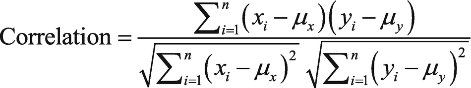
Say we have the data points x1, x2, . . ,xn from variable x and y1, y2, . . ,yn from the variable y. μx and μy are the mean values of the x and y variables, respectively. The mathematical formula in Figure 4-7 shows how to calculate correlation with this data.
Figure 4-7
Correlation
In PySpark SQL, we can calculate correlation using cov(col1, col2). This function takes two columns of the DataFrame at a time. The cov() function under the DataFrame and DataFrameStatFunctions classes are aliases of each other.
We have to find the following:
Correlation between iv1 and iv2.
Correlation between iv3 and iv1.
Correlation between iv2 and iv3.
How It Works
We are going to use the corrData DataFrame created in Recipe 4-7.
Step 4-9-1. Calculating Correlation Between Variables iv1 and iv2
Here is how we calculate the correlation between columns iv1 and iv2.
In [10]: corrData.corr('iv1','iv2')
Out[10]: 0.9999999999999998
Similarly, the correlation between other columns can be calculated in the following steps.
Step 4-9-2. Calculating Correlation Between Variables iv3 and iv1
In [11]: corrData.corr('iv1','iv3')
Out[11]: 0.9999999999999998
Step 4-9-3. Calculating Correlation Between Variables iv2 and iv3
In [12]: corrData.corr('iv2','iv3')
Out[12]: 1.0
Recipe 4-10. Describe a DataFrame
Problem
You want to calculate the summary statistics on all the columns in a DataFrame.
Solution
In Recipe 4-7, we learned how to calculate different summary statistics using DataFrame’s built-in aggregation functions.
PySpark SQL has provided two more very robust and easy-to-use functions, which calculate a group of summary statistics for each column. These functions are called describe() and summary().
The describe() function, which is defined on a DataFrame, calculates min, max, count, mean, and stddev for each column. For columns with categorical values, the describe() function returns count, min, and max for each categorical column. This function is used for exploratory data analysis. We can apply the describe() function on a single column or on columns. If no input is given, this function applies the summary statistics on each column and returns the result as a new DataFrame.
The summary() function calculates the summary statistics min, max, count, mean, and stddev, which is similar to the describe() function. Apart from this, the summary() function calculates the median and the 25 and 50 percentiles.
The describe() function takes columns as its input. It calculates specified summary statistics for each input. On the other hand, the summary() function takes the summary statistic names as Python strings and returns the summary statistics on each column that we provided as an argument.
We are going to use the corrData DataFrame we created in Recipe 4-7. We want to perform the following:
Apply the describe() function on each column.
Apply the describe() function on columns iv1 and iv2.
Add a column of a categorical variable to the corrData DataFrame and apply the describe() function on the categorical column.
Apply the summary() function on each column.
Apply the summary() function on columns iv2 and iv3.
How It Works
Step 4-10-1. Applying the describe( ) Function on Each Column
We are going to apply the describe() function on each column of the DataFrame. If there is no input to the describe function, it will be applied on every column.
In [1]: dataDescription = corrData.describe()
In [2]: dataDescription.show()
Here is the output:
+-------+--------+---------+--------+
|summary| iv1| iv2| iv3|
+-------+--------+---------+--------+
| count| 15| 15| 15|
| mean| 6.04466| 9.04466| 10.0446|
| stddev|0.495073|0.4950738|0.495073|
| min| 5.17| 8.17| 9.17|
| max| 6.89| 9.89| 10.89|
+-------+--------+---------+--------+
The describe() function returns the summary statistics. In the first column of the result, we can see all the summary statistic names. The second column, named iv1, provides values for the summary statistics values. The first value 15 in column iv1 is the number of elements in column iv1. Similarly, the second value 6.044666 in column iv1 is the mean value of data in that column. PySpark SQL will return a mean value with many decimal points. Some part of the mean result has been truncated, so it should be readable here.
Step 4-10-2. Applying the describe( ) Function on Columns iv1 and iv2
We can apply the describe() function with column selection. Here, we are going to apply the describe() function on columns iv1 and iv2.
In [3]: dataDescriptioniv1iv2 = corrData.describe(['iv1', 'iv2'])
In [4]: dataDescriptioniv1iv2.show()
Here is the output:
+-------+--------+---------+
|summary| iv1| iv2|
+-------+--------+---------+
| count| 15| 15|
| mean| 6.04466| 9.04466|
| stddev|0.495073|0.4950738|
| min| 5.17| 8.17|
| max| 6.89| 9.89|
+-------+--------+---------+
Can we apply selective summary statistics like mean and variance on columns? Not using the describe() function. In order to provide selective summary statistics, we have to use the summary() function.
Step 4-10-3. Applying the summary( ) Function on Each Column
As we have discussed, the summary() function is similar to the describe() function. The summary() function provides 25, 50, and 75 quantiles. In order to apply the summary() function to our summary statistics, we don’t provide any input.
In [5]: summaryData = corrData.summary()
In [6]: summaryData.show()
Here is the output:
+-------+--------+---------+--------+
|summary| iv1| iv2| iv3|
+-------+--------+---------+--------+
| count| 15| 15| 15|
| mean| 6.04466| 9.04466| 10.0446|
| stddev|0.495073|0.4950738|0.495073|
| min| 5.17| 8.17| 9.17|
| 25%| 5.64| 8.64| 9.64|
| 50%| 6.1| 9.1| 10.1|
| 75%| 6.32| 9.32| 10.32|
| max| 6.89| 9.89| 10.89|
+-------+--------+---------+--------+
Using the summary() function, we can apply selective summary statistics. The following line of code determines the mean and maximum value using the summary() function.
In [7]: summaryMeanMax = corrData.summary(['mean','max'])
In [8]: summaryMeanMax.show()
Here is the output:
+-------+-------+-------+-------+
|summary| iv1| iv2| iv3|
+-------+-------+-------+-------+
| mean|6.04466|9.04466|10.0446|
| max| 6.89| 9.89| 10.89|
+-------+-------+-------+-------+
Step 4-10-4. Applying the summary( ) Function on Columns iv2 and iv3
In order to apply the summary() function on selective columns, we have to first select the required columns using the select() function. Then, on selected columns, we can apply the summary() function.
In [9]: summaryiv1iv2 = corrData.select('iv1','iv2').summary('min','max')
We select columns iv1 and iv2 using the select() function and then apply the summary() function to calculate the minimum value and maximum value on the selected columns.
In [10]: summaryiv1iv2.show()
Here is the output:
+-------+----+----+
|summary| iv1| iv2|
+-------+----+----+
| min|5.17|8.17|
| max|6.89|9.89|
+-------+----+----+
Step 4-10-5. Adding a Column of Categorical Variables
We can add a column of categorical variables to the corrData DataFrame and then apply the describe() function on that categorical column.
You already know how the describe() function can be applied on numerical data. But you might want to know the behavior of the describe() function on the categorical variable. Categorical values are strings. We can find the minimum and maximum value of the categorical data. Apart from minimum and maximum, we can also determine the number of elements.
Now, we are going to create a UDF called labelIt(). The input of the labelIt function will be the values in column iv3. The UDF is going to return High if the input is greater than 10.0. Otherwise, it will return Low.
In [11]: from pyspark.sql.functions import udf
In [12]: def labelIt(x):
...: if x > 10.0 :
...: return 'High'
...: else:
...: return 'Low'
In [13]: labelIt = udf(labelIt)
We have now created the labelIt() UDF. The output of this UDF will constitute elements in the iv4 column in the newly created DataFrame, called corrData1.
In [14]: corrData1 = corrData.withColumn('iv4', labelIt('iv3'))
In [15]: corrData1.show(5)
Here is the output:
+----+----+-----+----+
| iv1| iv2| iv3| iv4|
+----+----+-----+----+
| 5.5| 8.5| 9.5| Low|
|6.13|9.13|10.13|High|
|5.92|8.92| 9.92| Low|
|6.89|9.89|10.89|High|
|6.12|9.12|10.12|High|
+----+----+-----+----+
only showing top 5 rows
The corrData1 DataFrame has an extra column at the end, called iv4. This column has categorical values of Low and High. We are going to apply summaries on each column of the DataFrame.
In [16]: meanMaxSummary = corrData1.summary('mean','max')
In [17]: meanMaxSummary.show()
Here is the output:
+-------+---------+---------+--------+----+
|summary| iv1| iv2| iv3| iv4|
+-------+---------+---------+--------+----+
| mean|6.0446666|9.0446666|10.04466|null|
| max| 6.89| 9.89| 10.89| Low|
+-------+---------+---------+--------+----+
Now the others:
In [18]: countMinMaxSummary = corrData1.summary('count','min','max')
In [19]: countMinMaxSummary.show()
+-------+----+----+-----+----+
|summary| iv1| iv2| iv3| iv4|
+-------+----+----+-----+----+
| count| 15| 15| 15| 15|
| min|5.17|8.17| 9.17|High|
| max|6.89|9.89|10.89| Low|
+-------+----+----+-----+----+
Recipe 4-11. Sort Data in a DataFrame
Problem
You want to sort records in a DataFrame.
Solution
You need to perform sorting operations from time to time, to sort the data for yourself or when some mathematical or statistical algorithm requires that the input be in sorted order. Sorting can be applied in increasing or decreasing order relative to some key or column.
The PySpark SQL API orderBy(*cols, **kwargs) can be used to sort records. It returns a new DataFrame, sorted by specified columns. We specify columns as the *cols argument of the function. The * in *cols is for the variable number of arguments and we are going to provide different columns as strings. The second argument **kwargs is a key/value pair. We are going to provide ascending as the key and its associated value as a Boolean or a list of Booleans. If we provide a list of Booleans as a value of the ascending key, the number of lists must be equal to the number of columns we provided in the cols argument.
We are going to perform sorting operations on a DataFrame we created in Recipe 4-1, that is swimmerDf. Let’s look at the Rows of swimmerDf to refresh our memory.
In [1]: swimmerDf.show(4)
+---+------+-----------+----------------+
| id|Gender| Occupation|swimTimeInSecond|
+---+------+-----------+----------------+
|id1| Male| Programmer| 16.73|
|id2|Female| Manager| 15.56|
|id3| Male| Manager| 15.15|
|id4| Male|RiskAnalyst| 15.27|
+---+------+-----------+----------------+
only showing top 4 rows
We have to perform the following:
Sort the swimmerDf DataFrame on the swimTimeInSecond column in ascending order.
Sort the swimmerDf DataFrame on the swimTimeInSecond column in descending order.
Sort the swimmerDf DataFrame on the Occupation and swimTimeInSecond columns in descending and ascending order, respectively.
Note
We can also use the sort() function in place of the orderBy() function.
How It Works
Step 4-11-1. Sorting a DataFrame in Ascending Order
We will sort the swimmerDf DataFrame on the swimTimeInSecond column in ascending order. The default value of the ascending argument is True. So, the following line of code will do what we need.
In [2]: swimmerDfSorted1 = swimmerDf.orderBy("swimTimeInSecond")
In [3]: swimmerDfSorted1.show(6)
Here is the output:
+----+------+-----------+----------------+
| id|Gender| Occupation|swimTimeInSecond|
+----+------+-----------+----------------+
| id3| Male| Manager| 15.15|
| id4| Male|RiskAnalyst| 15.27|
| id2|Female| Manager| 15.56|
| id5| Male| Programmer| 15.65|
| id6| Male|RiskAnalyst| 15.74|
|id12|Female|RiskAnalyst| 15.9|
+----+------+-----------+----------------+
only showing top 6 rows
We know that the default of ascending is True, but let’s print this value and we will get the same result.
In [4]: swimmerDf.orderBy("swimTimeInSecond", ascending=True).show(6)
Here is the output:
+----+------+-----------+----------------+
| id|Gender| Occupation|swimTimeInSecond|
+----+------+-----------+----------------+
| id3| Male| Manager| 15.15|
| id4| Male|RiskAnalyst| 15.27|
| id2|Female| Manager| 15.56|
| id5| Male| Programmer| 15.65|
| id6| Male|RiskAnalyst| 15.74|
|id12|Female|RiskAnalyst| 15.9|
+----+------+-----------+----------------+
only showing top 6 rows
Step 4-11-2. Sorting a DataFrame in Descending Order
Here, we will sort the swimmerDf DataFrame on the swimTimeInSecond column in descending order. For descending order, we have to set the ascending key to False.
In [5]: swimmerDfSorted2 =swimmerDf.orderBy("swimTimeInSecond", ascending=False)
In [6]: swimmerDfSorted2.show(6)
Here is the output:
+----+------+-----------+----------------+
| id|Gender| Occupation|swimTimeInSecond|
+----+------+-----------+----------------+
| id8| Male| Manager| 17.11|
| id9|Female| Programmer| 16.83|
| id7|Female| Programmer| 16.8|
| id1| Male| Programmer| 16.73|
|id10|Female|RiskAnalyst| 16.34|
|id11| Male| Programmer| 15.96|
+----+------+-----------+----------------+
only showing top 6 rows
Step 4-11-3. Sorting on Two Columns in Different Order
Here, we sort the swimmerDf DataFrame on the Occupation and swimTimeInSecond columns in descending and ascending order, respectively. In this case, the value of the ascending key is a list, that is [False,True].
In [7]: swimmerDfSorted3 = swimmerDf.orderBy("Occupation","swimTimeInSecond", ascending=[False,True])
In [8]: swimmerDfSorted3.show(6)
Here is the output:
+----+------+-----------+----------------+
| id|Gender| Occupation|swimTimeInSecond|
+----+------+-----------+----------------+
| id4| Male|RiskAnalyst| 15.27|
| id6| Male|RiskAnalyst| 15.74|
|id12|Female|RiskAnalyst| 15.9|
|id10|Female|RiskAnalyst| 16.34|
| id5| Male| Programmer| 15.65|
|id11| Male| Programmer| 15.96|
+----+------+-----------+----------------+
only showing top 6 rows
Recipe 4-12. Sort Data Partition-Wise
Problem
You want to sort a DataFrame partition-wise.
Solution
We know that DataFrames are partitioned over many nodes. Now we want to sort a DataFrame partition-wise. We are going to use the swimmerDf DataFrame, which we have used in previous recipes.
In PySpark SQL, partition-wise sorting that’s specified by columns is executed using the sortWithinPartitions(*cols, **kwargs) function. The sortWithinPartitions() function returns a new DataFrame. Arguments are similar to the orderBy() function’s argument.
We have to perform the following:
Perform a partition-wise sort on the swimmerDf DataFrame. We do this on the Occupation and swimTimeInSecond columns in descending and ascending order, respectively.
How It Works
Step 4-12-1. Performing a Partition-Wise Sort (Single Partition Case)
In this step, we sort on the swimmerDf DataFrame on the Occupation and swimTimeInSecond columns in descending and ascending order, respectively. To start, we apply the sortWithinPartitions() function:
In [1]: sortedPartitons = swimmerDf.sortWithinPartitions("Occupation","swimTimeInSecond", ascending=[False,True])
In [2]: swimmerDf1.show(6)
Here is the output:
+----+------+-----------+----------------+
| id|Gender| Occupation|swimTimeInSecond|
+----+------+-----------+----------------+
| id4| Male|RiskAnalyst| 15.27|
| id6| Male|RiskAnalyst| 15.74|
|id12|Female|RiskAnalyst| 15.9|
|id10|Female|RiskAnalyst| 16.34|
| id5| Male| Programmer| 15.65|
|id11| Male| Programmer| 15.96|
+----+------+-----------+----------------+
only showing top 6 rows
It seems that we have achieved the result. But why is this result similar to the result we got in Step 4-11-3 from Recipe 4-11? Let’s check on the number of partitions in this DataFrame. The following line of code shows that it is a single partitioned DataFrame.
Here, we again perform a sort on the swimmerDf DataFrame, on the Occupation and swimTimeInSecond columns, in descending and ascending order, respectively
Now let’s repartition the DataFrame into two partitions. Repartitioning a DataFrame can be done using the repartition() function, which looks like repartition(numPartitions, *cols). The first argument is the number of partitions and the second argument is the partitioning expressions. The repartition() function shuffles the data. It uses a hash partitioner to shuffle the data across the cluster. Repartitioning and shuffling are shown in Figure 4-8.
Figure 4-8
Repartitioning and shuffling
Figure 4-8 displays that the DataFrame on the left is partitioned into two parts—Partition 1 and Partition 2. A close look at Partition 1 and Partition 2 reveals that the DataFrame is not partitioned simply. Rather, the data has been shuffled. Let’s investigate repartitioning using the PySpark SQL API.
The results depict that the DataFrame has been repartitioned into two parts. Now it’s time to perform partition-wise sorting. But before we write the code for partition-wise sorting, let’s look at the process of sorting on repartitioned data.
Figure 4-9 displays the partition-wise sorting. Just concentrate on the left side and the right side Partition 1 DataFrame partition. In the process of sorting, nothing was shuffled. While sorting, each partition was considered an independent, full DataFrame.
Figure 4-9
Partitioning and sorting
In [7]: sortedPartitons = swimmerDf1.sortWithinPartitions("Occupation","swimTimeInSecond", ascending=[False,True])
This output should make the concept very clear. The records with id column values id10, id5, id11, id1, id7, and id3 are in the first partition and the rest are in the second partition.
Recipe 4-13. Remove Duplicate Records from a DataFrame
Problem
You want to remove duplicate records from a DataFrame.
Solution
In order to remove duplicates, we are going to use the drop_duplicates() function. This function can remove duplicated data conditioned on some column. If no column is specified as input, all the records in all the columns are checked.
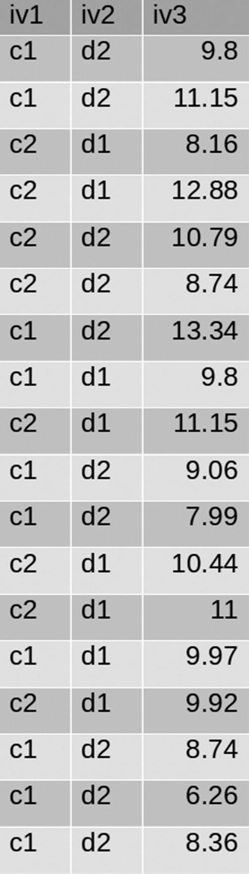
Figure 4-10 shows that some records are duplicates. If we conditioned duplicate removal on columns iv1 and iv2 we can see that many records are duplicates. We have to perform the following:
Figure 4-10
Sample data
Remove all the duplicate records.
Remove all the duplicate records conditioned on column iv1.
Remove all the duplicate records conditioned on columns iv1 and iv2.
How It Works
Step 4-13-1. Removing Duplicate Records
We are going to read our data from the ORC file duplicateData.
In [1]: duplicateDataDf = spark.read.orc(path='duplicateData')
In [2]: duplicateDataDf.show(6)
Here is the output:
+---+---+-----+
|iv1|iv2| iv3|
+---+---+-----+
| c1| d2| 9.8|
| c1| d2| 8.36|
| c1| d2| 9.06|
| c1| d2|11.15|
| c1| d2| 6.26|
| c2| d2| 8.74|
+---+---+-----+
only showing top 6 rows
We have created the DataFrame successfully. Now, we are going to drop all the duplicate records. We can see that there are 20 records in this DataFrame. We can verify the number of records using the count function, as follows.
In [3]: duplicateDataDf.count()
Here is the output:
Out[3]: 20
Let’s drop all the duplicate records.
In [4]: noDuplicateDf1 = duplicateDataDf.drop_duplicates()
In [5]: noDuplicateDf1.show()
Here is the output:
+---+---+-----+
|iv1|iv2| iv3|
+---+---+-----+
| c1| d2| 9.8|
| c1| d2|11.15|
| c2| d1| 8.16|
| c2| d1|12.88|
| c2| d2|10.79|
| c2| d2| 8.74|
| c1| d2|13.34|
| c1| d1| 9.8|
| c2| d1|11.15|
| c1| d2| 9.06|
| c1| d2| 7.99|
| c2| d1|10.44|
| c2| d1| 11.0|
| c1| d1| 9.97|
| c2| d1| 9.92|
| c1| d2| 8.74|
| c1| d2| 6.26|
| c1| d2| 8.36|
+---+---+-----+
In [6]: noDuplicateDf1.count()
Here is the output:
Out[6]: 18
It is clear that the total number of records after duplicate removal is 18. The duplicate data has been removed.
Step 4-13-2. Removing the Duplicate Records Conditioned on column iv1
From the duplicateDataDf DataFrame it is clear that column iv1 has two values—c1 and c2. Therefore, the final DataFrame, after duplicate removal, will have only two records. The first record will be c1 and the second record will be c2.
In [7]: noDuplicateDf2 = duplicateDataDf.drop_duplicates(['iv1'])
In [8]: noDuplicateDf2.show()
Here is the output:
+---+---+----+
|iv1|iv2| iv3|
+---+---+----+
| c1| d2| 9.8|
| c2| d2|8.74|
+---+---+----+
The noDuplicateDf2 DataFrame shows only two records. The first record has c1 in its iv1 column and the second record has c2 in the iv1 column.
Step 4-13-3. Removing the Duplicate Records Conditioned on Columns iv1 and iv2
The iv1 column has two distinct values—c1 and c2. Similarly, column iv2 has two distinct values—d1 and d2. That makes four distinct combinations and those are (c1, d1), (c1, d2), (c3, d3), and (c4, d4). Therefore, if we drop the duplicates conditioned on column iv1 and iv2, the final result will show four records.
In [9]: noDuplicateDf3 = duplicateDataDf.drop_duplicates(['iv1','iv2'])
In [10]: noDuplicateDf3.show()
Here is the output:
+---+---+----+
|iv1|iv2| iv3|
+---+---+----+
| c2| d1|9.92|
| c1| d2| 9.8|
| c2| d2|8.74|
| c1| d1|9.97|
+---+---+----+
In the final output, we have four records, as expected from this discussion.
Recipe 4-14. Sample Records
Problem
You want to sample some records from a given DataFrame.
Solution
Working on huge amounts of data is time-intensive and computation-intensive, even for a framework like PySpark. Sometimes data scientists instead get samples of data from an actual dataset and apply data science operations on that.
PySpark SQL provides tools that can gather sample from a given dataset. There are two DataFrame functions that can be applied to get samples from DataFrames. The first function—sample(withReplacement, fraction, seed=None)—returns a sample from a DataFrame. This function returns a new DataFrame. Its first argument, withReplacement, specifies that, if you need duplicate records in sampled data, the second argument fraction is the sampling fraction. Since that sample is taken randomly using some random number mechanism, the seed is used in the random number generation internally.
The second function—sampleBy(col, fractions, seed=None)—will perform stratified sampling conditioned on some column of the DataFrame which we provide as the col argument. The fractions argument is used to provide a sample fraction of each strata. This argument takes its value as a dictionary. The seed argument has the same meaning as before. See Figure 4-11.
Figure 4-11
Sample data
We are going to use the noDuplicateDf1 DataFrame that we created in Recipe 4-13. We have to perform the following:
Sample data from the noDuplicateDf1 DataFrame without replacement.
Sample data from the noDuplicateDf1 DataFrame with replacement.
Sample data from the noDuplicateDf1 DataFrame conditioned on the first column, called iv1.
How It Works
Step 4-14-1. Sampling Data from the noDuplicateDf1 DataFrame Without Replacement
Let’s print some records from the noDuplicateDf1 DataFrame, since this will refresh our memory about the DataFrame structure.
In [1]: noDuplicateDf1.show(6)
Here is the output:
+---+---+-----+
|iv1|iv2| iv3|
+---+---+-----+
| c1| d2| 9.8|
| c1| d2|11.15|
| c2| d1| 8.16|
| c2| d1|12.88|
| c2| d2|10.79|
| c2| d2| 8.74|
+---+---+-----+
only showing top 6 rows
We know from the previous recipe that it has 18 records.
In [2]: noDuplicateDf1.count()
Here is the output:
Out[2]: 18
We are going to fetch 50% of the records as a sample without replacement.
In [3]: sampleWithoutKeyConsideration = noDuplicateDf1.sample(withReplacement=False, fraction=0.5, seed=200)
In [4]: sampleWithoutKeyConsideration.show()
Here is the output:
+---+---+-----+
|iv1|iv2| iv3|
+---+---+-----+
| c1| d2| 9.8|
| c1| d2|11.15|
| c2| d1|12.88|
| c2| d2|10.79|
| c2| d2| 8.74|
| c2| d1| 11.0|
| c1| d1| 9.97|
| c1| d2| 6.26|
+---+---+-----+
Now we do the count:
In [5]: sampleWithoutKeyConsideration.count()
Here is the output:
Out[5]: 8
We fetched eight records in our sample DataFrame sampleWithoutKeyConsideration. The total number of records in the parent DataFrame noDuplicateDf1 is 18. We have asked for 50%, which means nine records, but we have only eight records. Remember that the output of the sample() function does not follow the exact fraction value.
Step 4-14-2. Sampling Data from the noDuplicateDf1 DataFrame with Replacements
In the following line of code, we provide the value of the withReplacement argument in the sample function as True. Due to this, we are going to get duplicate records in the output.
In [6]: sampleWithoutKeyConsideration1 = noDuplicateDf1.sample(withReplacement=True, fraction=0.5, seed=200)
In [7]: sampleWithoutKeyConsideration1.count()
Here is the output:
Out[7]: 6
In [8]: sampleWithoutKeyConsideration1.show()
Here is the output:
+---+---+-----+
|iv1|iv2| iv3|
+---+---+-----+
| c1| d2|13.34|
| c1| d2|13.34|
| c1| d2|13.34|
| c2| d1|10.44|
| c2| d1| 11.0|
| c1| d2| 8.74|
+---+---+-----+
As expected, the first three records are the same (duplicates of each other) in the sampleWithoutKeyConsideration1 DataFrame output.
Step 4-14-3. Sampling Data from the noDuplicateDf1 DataFrame Conditioned on the iv1 Column
Column iv1 has two values—c1 and c2. To perform stratified sampling, we have to use the sampleBy() function. Now we are going to condition on column iv1, which we are providing as a value of the argument col to the sampleBy() function. We are looking for equal representatives in output DataFrame from strata c1 and c2. Therefore, we have provided {'c1':0.5, 'c2':0.5} as the value of fractions.
In [9]: sampleWithKeyConsideration = noDuplicateDf1.sampleBy(col='iv1', fractions={'c1':0.5, 'c2':0.5},seed=200)
In [10]: sampleWithKeyConsideration.show()
+---+---+-----+
|iv1|iv2| iv3|
+---+---+-----+
| c1| d2| 9.8|
| c1| d2|11.15|
| c2| d1|12.88|
| c2| d2|10.79|
| c2| d2| 8.74|
| c2| d1| 11.0|
| c1| d1| 9.97|
| c1| d2| 6.26|
+---+---+-----+
We can observe an equal number of representatives from strata c1 and c2.
Recipe 4-15. Find Frequent Items
Problem
You want to determine which items appear most frequently in the columns of the DataFrame.
Solution
In order to see the frequent items, we are going to use the freqItems() function.
How It Works
First we are going to calculate the frequent items in column iv1.
In [1]: duplicateDataDf.freqItems(cols=['iv1']).show()
Here is the output:
+-------------+
|iv1_freqItems|
+-------------+
| [c1, c2]|
+-------------+
Now we are going to determine the frequent items in the iv1 and iv2 columns.
In [2]: duplicateDataDf.freqItems(cols=['iv1','iv2']).show()