© Raju Kumar Mishra and Sundar Rajan Raman 2019
Raju Kumar Mishra and Sundar Rajan RamanPySpark SQL Recipeshttps://doi.org/10.1007/978-1-4842-4335-0_5

5. Data Merging and Data Aggregation Using PySparkSQL

Raju Kumar Mishra1  and Sundar Rajan Raman2
(1)
Bangalore, Karnataka, India
(2)
Chennai, Tamil Nadu, India
 
Data merging and data aggregation are an essential part of the day-to-day activities of PySparkSQL users. This chapter will discuss and describe the following recipes.
  • Recipe 5-1. Aggregate data on a single key

  • Recipe 5-2. Aggregate data on multiple keys

  • Recipe 5-3. Create a contingency table

  • Recipe 5-4. Perform joining operations on two DataFrames

  • Recipe 5-5. Vertically stack two DataFrames

  • Recipe 5-6. Horizontally stack two DataFrames

  • Recipe 5-7. Perform missing value imputation

Recipe 5-1. Aggregate Data on a Single Key

Problem

You want to perform data aggregation on a DataFrame, grouped on a single key.

Solution

We perform data aggregation to observe summary of data.

The data has been taken from an R datasets package. The name of the data is UCBAdmissions. This dataset is in the form of R tables. I transformed it into tabular form and saved it in a table of a MySQL database. We have to read this table using PySparkSQL and perform the following:
  • Mean value of the number of accepted and rejected students

  • Mean value of students gender-wise who have applied for admission

  • The average frequency of application gender-wise

In order to run the aggregation API, we have to first group the data if the aggregation has to be done on some column. In order to group a column based on a data condition, we have to use the groupby() function . After grouping the data, we can apply the following aggregation functions to it.
  • mean()

  • count()

  • sum()

  • min()

  • max()

  • etc ….

How It Works

Step 5-1-1. Reading the Data from MySQL

The admission data is in the ucbdata table of the pysparksqlbook database of MySQL. We can read it using the following line of code.
In [1]: dbURL = "jdbc:mysql://localhost/pysparksqlbook"
In [2]: ucbDataFrame = spark.read.format("jdbc").options(url = dbURL, database ='pysparksqlbook', dbtable ='ucbdata', user="root", password="").load();
In [3]: ucbDataFrame.show()
Here is the output:
+--------+------+----------+---------+
|   admit|gender|department|frequency|
+--------+------+----------+---------+
|Admitted|  Male|         A|      512|
|Rejected|  Male|         A|      313|
|Admitted|Female|         A|       89|
|Rejected|Female|         A|       19|
|Admitted|  Male|         B|      353|
|Rejected|  Male|         B|      207|
|Admitted|Female|         B|       17|
|Rejected|Female|         B|        8|
|Admitted|  Male|         C|      120|
|Rejected|  Male|         C|      205|
|Admitted|Female|         C|      202|
|Rejected|Female|         C|      391|
|Admitted|  Male|         D|      138|
|Rejected|  Male|         D|      279|
|Admitted|Female|         D|      131|
|Rejected|Female|         D|      244|
|Admitted|  Male|         E|       53|
|Rejected|  Male|         E|      138|
|Admitted|Female|         E|       94|
|Rejected|Female|         E|      299|
+--------+------+----------+---------+
only showing top 20 rows

Step 5-1-2. Calculating the Required Means

We need the mean value of the number of accepted and admitted students. We are going to group data on the admit column using the groupby() function. Thereafter, we are going to apply the mean() function.
In [4]: groupedOnAdmit = ucbDataFrame.groupby(["admit"]).mean()
In [5]: groupedOnAdmit.show()
Here is the output:
+--------+------------------+
|   admit|    avg(frequency)|
+--------+------------------+
|Rejected|230.91666666666666|
|Admitted|            146.25|
+--------+------------------+

Step 5-1-3. Grouping by Gender

Now we want the mean value of students gender-wise who have applied for admission. We are going to group data on the gender column using the groupby() function. Thereafter, we are going to apply the mean() function.
In [6]: groupedOnGender = ucbDataFrame.groupby(["gender"]).mean()
In [7]: groupedOnGender.show()
Here is the output:
+------+------------------+
|gender|    avg(frequency)|
+------+------------------+
|Female|152.91666666666666|
|  Male|            224.25|
+------+------------------+

Step 5-1-4. Finding the Average Frequency of Application by Gender

We are going to group the data on the department column using the groupby() function. Thereafter, we are going to apply the mean() function.
In [8]: groupedOnDepartment = ucbDataFrame.groupby(["department"]).mean()
In [9]: groupedOnDepartment.show()
+----------+--------------+
|department|avg(frequency)|
+----------+--------------+
|         F|         178.5|
|         E|         146.0|
|         B|        146.25|
|         D|         198.0|
|         C|         229.5|
|         A|        233.25|
+----------+--------------+

Recipe 5-2. Aggregate Data on Multiple Keys

Problem

You want to perform data aggregation on a DataFrame, grouped on multiple keys.

Solution

We are going to use the admission data from the previous recipe. In order to aggregate data conditioned on multiple columns, we have to group it on multiple columns. We can use the groupby() function to group data conditioned on multiple columns. We do this with the following steps:
  • Group the data on the admit and gender columns and find the mean of applications to the college.

  • Group the data on the admit and department columns and find the mean of applications to the college.

How It Works

Let’s print the UCB admission data.
In [1]: ucbDataFrame.show()
Here is the output:
+--------+------+----------+---------+
|   admit|gender|department|frequency|
+--------+------+----------+---------+
|Admitted|  Male|         A|      512|
|Rejected|  Male|         A|      313|
|Admitted|Female|         A|       89|
|Rejected|Female|         A|       19|
|Admitted|  Male|         B|      353|
|Rejected|  Male|         B|      207|
|Admitted|Female|         B|       17|
|Rejected|Female|         B|        8|
|Admitted|  Male|         C|      120|
|Rejected|  Male|         C|      205|
|Admitted|Female|         C|      202|
|Rejected|Female|         C|      391|
|Admitted|  Male|         D|      138|
|Rejected|  Male|         D|      279|
|Admitted|Female|         D|      131|
|Rejected|Female|         D|      244|
|Admitted|  Male|         E|       53|
|Rejected|  Male|         E|      138|
|Admitted|Female|         E|       94|
|Rejected|Female|         E|      299|
+--------+------+----------+---------+
only showing top 20 rows

Step 5-2-1. Grouping the Data on Gender and Finding the Mean of Applications

We are going to group the data on the admit and gender columns using the groupby() function. Thereafter, we are going to apply the mean() function.
In [2]: groupedOnAdmitGender =ucbDataFrame.groupby( [ "admit" , "gender  "]  ).mean( )
In [3]: groupedOnAdmitGender.show()
Here is the output:
+--------+------+------------------+
|   admit|gender|    avg(frequency)|
+--------+------+------------------+
|Rejected|Female|             213.0|
|Rejected|  Male|248.83333333333334|
|Admitted|Female| 92.83333333333333|
|Admitted|  Male|199.66666666666666|
+--------+------+------------------+

Step 5-2-2. Grouping the Data on Department and Finding the Mean of Applications

We are going to group the data on the admit and department columns using the groupby() function. Thereafter, we are going to apply the mean() function.
In [4]: groupedOnAdmitDepartment = ucbDataFrame.groupby([ "admit", "department" ]).mean()
In [5]: groupedOnAdmitDepartment.show()
Here is the output:
+--------+----------+--------------+
|   admit|department|avg(frequency)|
+--------+----------+--------------+
|Admitted|         C|         161.0|
|Admitted|         E|          73.5|
|Rejected|         A|         166.0|
|Admitted|         B|         185.0|
|Admitted|         F|          23.0|
|Admitted|         A|         300.5|
|Rejected|         C|         298.0|
|Rejected|         D|         261.5|
|Admitted|         D|         134.5|
|Rejected|         F|         334.0|
|Rejected|         B|         107.5|
|Rejected|         E|         218.5|
+--------+----------+--------------+

Recipe 5-3. Create a Contingency Table

Problem

You want to create a contingency table.

Solution

Contingency tables are also known as cross tabulations. They show the pairwise frequency of the given columns.

The owner of a restaurant wants to know about the service provided. She surveys some customers and gets the result shown in Figure 5-1. This data is in a MongoDB collection called restaurantSurvey . We can observe it using the following MongoDB command.
> db.restaurantSurvey.find().pretty().limit(5)
../images/469054_1_En_5_Chapter/469054_1_En_5_Fig1_HTML.jpg
Figure 5-1

Contingency table for the restaurant survey

Here is the output:
{
    "_id" : ObjectId("5ba7e6a259acc01fedb4d78a"),
    "Gender" : "Male",
    "Vote" : "Yes"
}
{
    "_id" : ObjectId("5ba7e6a259acc01fedb4d78b"),
    "Gender" : "Male",
    "Vote" : "Yes"
}
{
    "_id" : ObjectId("5ba7e6a259acc01fedb4d78c"),
    "Gender" : "Male",
    "Vote" : "No"
}
{
    "_id" : ObjectId("5ba7e6a259acc01fedb4d78d"),
    "Gender" : "Male",
    "Vote" : "DoNotKnow"
}
{
    "_id" : ObjectId("5ba7e6a259acc01fedb4d78e"),
    "Gender" : "Male",
    "Vote" : "Yes"
}

We have to make a contingency table using the data in Figure 5-1.

How It Works

Step 5-3-1. Reading Restaurant Survey Data from MongoDB

The restaurant survey data is in a restaurantSurvey collection of the pysparksqlbook database in MongoDB. The following line of code will read our data from MongoDB.
In [1]: surveyDf = spark.read.format("com.mongodb.spark.sql.DefaultSource").option("uri","mongodb://127.0.0.1/pysparksqlbook.restaurantSurvey").load()
In [2]: surveyDf.show(5)
Here is the output:
+------+---------+--------------------+
|Gender|     Vote|                 _id|
+------+---------+--------------------+
|  Male|      Yes|[5ba7e6a259acc01f...|
|  Male|      Yes|[5ba7e6a259acc01f...|
|  Male|       No|[5ba7e6a259acc01f...|
|  Male|DoNotKnow|[5ba7e6a259acc01f...|
|  Male|      Yes|[5ba7e6a259acc01f...|
+------+---------+--------------------+
only showing top 5 rows
We have read our data. Since the _id column is not required, we are going to drop it.
In [3]: surveyDf = surveyDf.drop("_id")
In [4]: surveyDf.show(5)
Here is the output:
+------+---------+
|Gender|     Vote|
+------+---------+
|  Male|      Yes|
|  Male|      Yes|
|  Male|       No|
|  Male|DoNotKnow|
|  Male|      Yes|
+------+---------+
only showing top 5 rows

Step 5-3-2. Creating a Contingency Table

In order to create a contingency table, we have to use the crosstab() function. This function takes two columns as arguments.
In [5]: surveyDf.crosstab("Gender","Vote").show()
Here is the output:
+-----------+---------+--+---+
|Gender_Vote|DoNotKnow|No|Yes|
+-----------+---------+--+---+
|       Male|        2| 5|  5|
|     Female|        1| 1|  6|
+-----------+---------+--+---+

We have our contingency table.

Recipe 5-4. Perform Joining Operations on Two DataFrames

Problem

You want to perform a join operation on two DataFrames.

Solution

Data scientists often need to merge the content of two DataFrames using joining operations. For people who use SQL, DataFrame joining is the same as table joining. It is as simple as any other operation on DataFrames. We perform the following four types of joins on DataFrames.
  • Inner join

  • Left outer join

  • Right outer join

  • Full outer join

We have been given two tables in a Cassandra database. The data of first table is displayed in Figure 5-2. The first table is called students.
../images/469054_1_En_5_Chapter/469054_1_En_5_Fig2_HTML.jpg
Figure 5-2

The students table

The second table is shown in Figure 5-3. Its name is subjects.
../images/469054_1_En_5_Chapter/469054_1_En_5_Fig3_HTML.jpg
Figure 5-3

The subjects table

We have to perform the following.
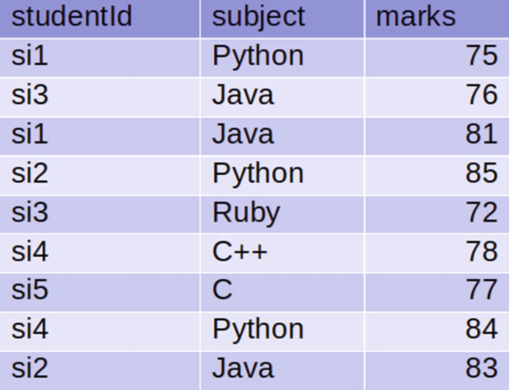
  • Read the students and subjects tables from the Cassandra database.

  • Perform an inner join on the DataFrames.

  • Perform an left outer join on the DataFrames.

  • Perform a right outer join on the DataFrames.

  • Perform a full outer join on the DataFrames.

In order to join the two DataFrames, PySparkSQL provides a join() function, which works on the DataFrames.

The join() function takes three arguments. The first argument, called other, is the other DataFrame. The second argument, called on, defines the key columns on which we want to perform joining operations. The third argument, called how, defines which join type to perform.

How It Works

Let’s explore this recipe in a step-by-step fashion.

Step 5-4-1. Reading Student and Subject Data Tables from a Cassandra Database

We need to read the students data in the pysparksqlbook keyspace of the students table. Similarly, we need to read the subjects data in the same keyspace, but in a Cassandra table called subjects.

The following lines will read the data tables from the Cassandra database.
In [1]: studentsDf = spark.read.format("org.apache.spark.sql.cassandra").options( keyspace="pysparksqlbook", table="students").load()
In [2]: subjectsDf = spark.read.format( "org.apache.spark.sql.cassandra").options( keyspace="pysparksqlbook", table="subjects").load()
After reading data from Cassandra, let’s print it and verify that we have created a DataFrame.
In [3]: studentsDf.show()
Here is the output:
+---------+------+-------+
|studentid|gender|   name|
+---------+------+-------+
|      si3|     F|  Julie|
|      si2|     F|  Maria|
|      si1|     M|  Robin|
|      si6|     M|William|
|      si4|     M|    Bob|
+---------+------+-------+
In [4]: subjectsDf.show()
Here is the output:
+--+-----+---------+--------+
|id|marks|studentid|subjects|
+--+-----+---------+--------+
| 6|   78|      si4|     C++|
| 9|   83|      si2|    Java|
| 5|   72|      si3|    Ruby|
| 4|   85|      si2|  Python|
| 7|   77|      si5|       C|
| 1|   75|      si1|  Python|
| 8|   84|      si4|  Python|
| 2|   76|      si3|    Java|
| 3|   81|      si1|    Java|
+--+-----+---------+--------+
We have created our DataFrames. The subjectsDf DataFrame contains a column called id, which is not required. We can drop it. To drop unwanted columns, use the drop() function .
In [5]: subjectsDf = subjectsDf.drop("id")
In [6]: subjectsDf.show()
Here is the output:
+-----+---------+--------+
|marks|studentid|subjects|
+-----+---------+--------+
|   78|      si4|     C++|
|   83|      si2|    Java|
|   72|      si3|    Ruby|
|   85|      si2|  Python|
|   77|      si5|       C|
|   75|      si1|  Python|
|   84|      si4|  Python|
|   76|      si3|    Java|
|   81|      si1|    Java|
+-----+---------+--------+

We have dropped the unwanted column.

Step 5-4-2. Performing an Inner Join on DataFrames

At this moment, we have two DataFrames called studentsDf and subjectsDf. We have to perform inner joins on these DataFrames. We have a studentid column that’s common in both DataFrames. We are going to perform an inner join on that studentid column.

Inner joins return records when key values in those records match. If we look at values in the studentid column in both DataFrames, we will find that the values si1, si2, si3, and si4 are common to both DataFrames. Therefore, an inner join will return records only for those values.
In [7]: innerDf = studentsDf.join(subjectsDf, studentsDf.studentid == subjectsDf.studentid, how= "inner")

Let’s explore the argument of the join() function. The first argument is subjectsDf, which is the DataFrame that’s getting joined with the studentsDf DataFrame. The second argument is studentsDf.studentid == subjectsDf.studentid, which indicates the condition of joining. The last argument tells us that we have to perform an inner join.

Let’s print the result.
In [8]: innerDf.show()
Here is the output:
+---------+------+-----+-----+---------+--------+
|studentid|gender| name|marks|studentid|subjects|
+---------+------+-----+-----+---------+--------+
|      si2|     F|Maria|   83|      si2|    Java|
|      si2|     F|Maria|   85|      si2|  Python|
|      si4|     M|  Bob|   78|      si4|     C++|
|      si4|     M|  Bob|   84|      si4|  Python|
|      si3|     F|Julie|   72|      si3|    Ruby|
|      si3|     F|Julie|   76|      si3|    Java|
|      si1|     M|Robin|   75|      si1|  Python|
|      si1|     M|Robin|   81|      si1|    Java|
+---------+------+-----+-----+---------+--------+

In the output DataFrame innerDf, we can observe that in the studentid column, we see only si1, si2, si3, and si4 .

Step 5-4-3. Performing a Left Outer Join on DataFrames

In this step of recipe, we are going to perform the left outer join on the DataFrames. In a left outer join, each key for the first DataFrame and matched keys from the second DataFrame will be in the result.

In our case, we are using studentsDf as the first DataFrame and subjectsDf as the second DataFrame when joining. So every value in the studentid column of studentsDf will be shown in the output. In the studentid column, we show si1, si2, si3, si4, and si6.
In [9]: leftOuterDf = studentsDf.join(subjectsDf, studentsDf.studentid == subjectsDf.studentid, how= "left")
It can be observed that the value of the third argument is left for the left outer join.
In [10]: leftOuterDf.show()
Here is the output:
+---------+------+-------+-----+---------+--------+
|studentid|gender|   name|marks|studentid|subjects|
+---------+------+-------+-----+---------+--------+
|      si2|     F|  Maria|   83|      si2|    Java|
|      si2|     F|  Maria|   85|      si2|  Python|
|      si4|     M|    Bob|   78|      si4|     C++|
|      si4|     M|    Bob|   84|      si4|  Python|
|      si3|     F|  Julie|   72|      si3|    Ruby|
|      si3|     F|  Julie|   76|      si3|    Java|
|      si6|     M|William| null|     null|    null|
|      si1|     M|  Robin|   75|      si1|  Python|
|      si1|     M|  Robin|   81|      si1|    Java|
+---------+------+-------+-----+---------+--------+

The studentid column in the resulting DataFrame shows si1, si2, si3, si4, and si6 .

Step 5-4-4. Performing a Right Outer Join on DataFrames

The following line of code will perform a right outer join. In order to perform a right join, the value the of the how argument will be right.
In [11]: rightOuterDf = studentsDf.join(subjectsDf, studentsDf.studentid == subjectsDf.studentid, how= "right")
In [12]: rightOuterDf.show()
Here is the output:
+---------+------+-----+-----+---------+--------+
|studentid|gender| name|marks|studentid|subjects|
+---------+------+-----+-----+---------+--------+
|     null|  null| null|   77|      si5|       C|
|      si2|     F|Maria|   83|      si2|    Java|
|      si2|     F|Maria|   85|      si2|  Python|
|      si4|     M|  Bob|   78|      si4|     C++|
|      si4|     M|  Bob|   84|      si4|  Python|
|      si3|     F|Julie|   72|      si3|    Ruby|
|      si3|     F|Julie|   76|      si3|    Java|
|      si1|     M|Robin|   75|      si1|  Python|
|      si1|     M|Robin|   81|      si1|    Java|
+---------+------+-----+-----+---------+--------+

The result of the right outer join is rightOuterDf .

Step 5-4-5. Performing a Full Outer Join on DataFrames

In a full outer join, all values from the studentid column of the two DataFrames will be in the result.
In [13]: outerDf = studentsDf.join(subjectsDf, studentsDf.studentid == subjectsDf.studentid, how= "outer")
In [14]: outerDf.show()
Here is the output:
+---------+------+-------+-----+---------+--------+
|studentid|gender|   name|marks|studentid|subjects|
+---------+------+-------+-----+---------+--------+
|     null|  null|   null|   77|      si5|       C|
|      si2|     F|  Maria|   83|      si2|    Java|
|      si2|     F|  Maria|   85|      si2|  Python|
|      si4|     M|    Bob|   78|      si4|     C++|
|      si4|     M|    Bob|   84|      si4|  Python|
|      si3|     F|  Julie|   72|      si3|    Ruby|
|      si3|     F|  Julie|   76|      si3|    Java|
|      si6|     M|William| null|     null|    null|
|      si1|     M|  Robin|   75|      si1|  Python|
|      si1|     M|  Robin|   81|      si1|    Java|
+---------+------+-------+-----+---------+--------+

Recipe 5-5. Vertically Stack Two DataFrames

Problem

You want to perform vertical stacking on two DataFrames.

Solution

Two or more DataFrames can be stacked, one above the other. This process is known as vertical stacking of DataFrames, and is shown in Figure 5-4.
../images/469054_1_En_5_Chapter/469054_1_En_5_Fig4_HTML.jpg
Figure 5-4

Vertically stacking DataFrames

Figure 5-4 depicts the vertical stacking of two DataFrames. On the left, we can see two DataFrames called dfOne and dfTwo. DataFrame dfOne consists of three columns and four rows. Similarly, DataFrame dfTwo also has three row and three columns. The right side of Figure 5-4 displays the DataFrame that’s been created by vertically stacking the dfOne and dfTwo DataFrames.

The firstverticaltable and secondverticaltable tables are in a PostgreSQL database. We can get the tables using the following SQL commands.
pysparksqldb=#  select * from firstverticaltable;
Here is the output:
  iv1|  iv2|  iv3
-----+-----+-----
    9|11.43|10.25
10.26| 8.35| 9.94
 9.84| 9.28| 9.22
11.77|10.18|11.02
(4 rows)
pysparksqldb=# select * from secondverticaltable ;
Here is the output:
  iv1|  iv2|  iv3
-----+-----+-----
   11|12.64|12.18
12.26|10.84|12.19
11.84|13.43| 11.6
(3 rows)
We have to perform the following:
  • We have to read two tables—firstverticaltable and secondverticaltable—from the PostgreSQL database and create DataFrames.

  • We have to vertically stack the newly created DataFrames.

We can perform vertical stacking using the union() function . The union() function takes only one input, and that is another DataFrame. This function is equivalent to UNION ALL in SQL. The resultant DataFrame of the union() function might have duplicate records. It is therefore suggested that we use the distinct() function on the result of a union() function .

How It Works

The first step is to read the data tables from PostgreSQL and create the DataFrames.

Step 5-5-1. Reading Tables from PostgreSQL

Note

In order to connect with the PostgreSQL database, we have to start a PySpark shell with the following options:

$pyspark --driver-class-path ~/.ivy2/jars/org.postgresql_postgresql-42.2.4.jar --packages org.postgresql:postgresql:42.2.4

Now it’s time to read our tables. Our tables are in pysparksqldb of a PostgreSQL database. The following line of code will read from PostgreSQL.
In [1]: dbURL = "jdbc:postgresql://localhost/pysparksqldb?user=postgres&password=""
In [1]: verticalDfOne = spark.read.format("jdbc").options(url = dbURL, database ='pysparksqldb', dbtable ='firstverticaltable').load();
In [2]: verticalDfOne.show()
Here is the output:
+-----+-----+-----+
|  iv1|  iv2|  iv3|
+-----+-----+-----+
|  9.0|11.43|10.25|
|10.26| 8.35| 9.94|
| 9.84| 9.28| 9.22|
|11.77|10.18|11.02|
+-----+-----+-----+
We have read the firstverticaltable table. Now let’s read another table.
In [3]: verticalDfTwo = spark.read.format("jdbc").options(url = dbURL, database ='pysparksqldb', dbtable ='secondverticaltable').load();
In [4]: verticalDfTwo.show()
Here is the output:
+-----+-----+-----+
|  iv1|  iv2|  iv3|
+-----+-----+-----+
| 11.0|12.64|12.18|
|12.26|10.84|12.19|
|11.84|13.43| 11.6|
+-----+-----+-----+

Step 5-5-2. Performing Vertical Stacking of Newly Created DataFrames

We have created two DataFrames, called verticalDfOne and verticalDfTwo. We are going to perform vertical stacking of these DataFrames using the union() function.
In [5]: vstackedDf = verticalDfOne.union(verticalDfTwo)
In [6]: vstackedDf.show()
Here is the output:
+-----+-----+-----+
|  iv1|  iv2|  iv3|
+-----+-----+-----+
|  9.0|11.43|10.25|
|10.26| 8.35| 9.94|
| 9.84| 9.28| 9.22|
|11.77|10.18|11.02|
| 11.0|12.64|12.18|
|12.26|10.84|12.19|
|11.84|13.43| 11.6|
+-----+-----+-----+

Finally, we have a vertically stacked DataFrame, named vstackedDf .

Recipe 5-6. Horizontally Stack Two DataFrames

Problem

You want to horizontally stack two DataFrames.

Solution

Horizontal stacking is less frequent in day-to-day work, but this does not decrease the importance of it. Figure 5-5 shows horizontal stacking of the tables called dfOne and dfTwo.
../images/469054_1_En_5_Chapter/469054_1_En_5_Fig5_HTML.jpg
Figure 5-5

Horizontally stacking DataFrames

We can observe from Figure 5-5 that horizontal stacking means putting DataFrames side by side. It is not easy in PySparkSQL, as there is no dedicated API for this task.

Since there is no dedicated API for horizontal stacking, we have to use other API to get the job done. How do we perform horizontal stacking? One way is to add a new column of row numbers in each DataFrame. After adding this new column of row numbers, we can perform an inner join to get the required DataFrames vertically stacked.

We have to perform the following:
  • We have to read two tables, called firsthorizontable and secondhorizontable, from the PostgreSQL database and create DataFrames.

  • We have to perform horizontal stacking of these newly created DataFrames.

We can observe our tables in PostgreSQL using the following commands.
pysparksqldb=# select * from firsthorizontable ;
Here is the output:
  iv1|  iv2|  iv3
-----+-----+-----
    9|11.43|10.25
10.26| 8.35| 9.94
 9.84| 9.28| 9.22
11.77|10.18|11.02
10.23|10.19| 8.17
(5 rows)
pysparksqldb=# select * from secondhorizontable;
Here is the output:
  iv4|  iv5|  iv6
-----+-----+-----
   11|12.64|12.18
12.26|10.84|12.19
11.84|13.43| 11.6
13.77|10.35|13.48
12.23|11.28|12.25
(5 rows)

How It Works

Note

In order to connect with the PostgreSQL database, we have to start a PySpark shell with the following options:

$pyspark --driver-class-path  ~/.ivy2/jars/org.postgresql_postgresql-42.2.4.jar  --packages org.postgresql:postgresql:42.2.4

Step 5-6-1. Reading Tables from PostgreSQL and Creating DataFrames

We have to read two tables from the PostgreSQL database. Let’s read these one by one.
In [1]: dbURL = "jdbc:postgresql://localhost/pysparksqldb?user=postgres&password=""
In [2]: horizontalDfOne = spark.read.format("jdbc").options(url = dbURL, database ='pysparksqldb', dbtable ='firsthorizontable').load();
In [3]: horizontalDfOne.show()
Here is the output:
+-----+-----+-----+
|  iv1|  iv2|  iv3|
+-----+-----+-----+
|  9.0|11.43|10.25|
|10.26| 8.35| 9.94|
| 9.84| 9.28| 9.22|
|11.77|10.18|11.02|
|10.23|10.19| 8.17|
+-----+-----+-----+
In [4]: horizontalDfTwo = spark.read.format("jdbc").options(url = dbURL, database ='pysparksqldb', dbtable ='secondhorizontable').load();
In [5]: horizontalDfTwo.show()
Here is the output:
+-----+-----+-----+
|  iv4|  iv5|  iv6|
+-----+-----+-----+
| 11.0|12.64|12.18|
|12.26|10.84|12.19|
|11.84|13.43| 11.6|
|13.77|10.35|13.48|
|12.23|11.28|12.25|
+-----+-----+-----+

Step 5-6-2. Performing Horizontal Stacking of Newly Created DataFrames

After creating the DataFrames, we have to add a new column to both. Both DataFrames need to have a new column that shows the integer sequence. We can create this new column using the monotonically_increasing_id() function. We can get this function from the pyspark.sql.functions submodule. Let’s import it.
In [5]: from pyspark.sql.functions import monotonically_increasing_id
In the following line of code, we are going to add a new column that contains a sequence of integers, starting from zero.
In [6]: horizontalDfOne = horizontalDfOne.withColumn("id", monotonically_increasing_id() )
In [7]: horizontalDfOne.show()
Here is the output:
+-----+-----+-----+--+
|  iv1|  iv2|  iv3|id|
+-----+-----+-----+--+
| 9.0 |11.43|10.25| 0|
|10.26| 8.35| 9.94| 1|
| 9.84| 9.28| 9.22| 2|
|11.77|10.18|11.02| 3|
|10.23|10.19| 8.17| 4|
+-----+-----+-----+--+
We have successfully added the new column of integer sequence to the horizontalDfOne DataFrame. The following line of code will add the same column to the horizontalDfTwo DataFrame .
In [8]: horizontalDfTwo = horizontalDfTwo.withColumn( "id",  monotonically_increasing_id() )
In [9]: horizontalDfTwo.show()
Here is the output:
+-----+-----+-----+--+
|  iv4|  iv5|  iv6|id|
+-----+-----+-----+--+
| 11.0|12.64|12.18| 0|
|12.26|10.84|12.19| 1|
|11.84|13.43| 11.6| 2|
|13.77|10.35|13.48| 3|
|12.23|11.28|12.25| 4|
+-----+-----+-----+--+
We are now going to perform an inner join on horizontalDfOne and horizontalDfTwo. An inner join is performed on the id column.
In [10]: hStackedDf = horizontalDfOne.join(horizontalDfTwo, horizontalDfOne.id == horizontalDfTwo.id, how="inner")
In [11]: hStackedDf.show()
Here is the output:
+-----+-----+-----+--+-----+-----+-----+--+
|  iv1|  iv2|  iv3|id|  iv4|  iv5|  iv6|id|
+-----+-----+-----+--+-----+-----+-----+--+
|  9.0|11.43|10.25| 0| 11.0|12.64|12.18| 0|
|10.26| 8.35| 9.94| 1|12.26|10.84|12.19| 1|
|11.77|10.18|11.02| 3|13.77|10.35|13.48| 3|
| 9.84| 9.28| 9.22| 2|11.84|13.43| 11.6| 2|
|10.23|10.19| 8.17| 4|12.23|11.28|12.25| 4|
+-----+-----+-----+--+-----+-----+-----+--+
After the inner join, we have our two DataFrames horizontally stacked and the results stored in hStackedDf. We are not in need of the id column. Therefore, we can drop it.
In [12]: hStackedDf = hStackedDf.drop("id")
In [13]: hStackedDf.show()
Here is the output:
+-----+-----+-----+-----+-----+-----+
|  iv1|  iv2|  iv3|  iv4|  iv5|  iv6|
+-----+-----+-----+-----+-----+-----+
|  9.0|11.43|10.25| 11.0|12.64|12.18|
|10.26| 8.35| 9.94|12.26|10.84|12.19|
|11.77|10.18|11.02|13.77|10.35|13.48|
| 9.84| 9.28| 9.22|11.84|13.43| 11.6|
|10.23|10.19| 8.17|12.23|11.28|12.25|
+-----+-----+-----+-----+-----+-----+

And finally we have our required result.

Recipe 5-7. Perform Missing Value Imputation

Problem

You want to perform missing value imputation in a DataFrame.

Solution

For the data scientist, missing values are inevitable. PySparkSQL provides tools to handle missing data in DataFrames. Two important functions that deal with missing or null values are dropna() and fillna().

In Figure 5-6, the contents of the DataFrame are displayed. We can observe that there are two missing values in row four and is one missing value in row two.
../images/469054_1_En_5_Chapter/469054_1_En_5_Fig6_HTML.jpg
Figure 5-6

DataFrame with missing values

The dropna() function can remove rows that contain null data. It takes three arguments. The first argument is how, and it can take two values—any or all. If the value of how is all, a row will be dropped only if all the values of the row are null. If the value of how is any, the row will be dropped if any of its values are null.

The second argument of the dropna() function is called thresh. The default value for thresh is None. It takes an integer value. The thresh argument overwrites the first argument, how. If thresh is set to the integer n, all rows where the number of non-null values is less than n will be dropped.

The last argument of the dropna() function is subset. This is an optional name of columns to be considered.

The second important function for dealing with null values is fillna(). The first argument is a value. The fillna() function will replace any null value with the value argument .

How It Works

Step 5-7-1. Reading Data from MongoDB

We have a table called missingData in the pysparksqlbook database of MongoDB. We have to start the PySpark shell using a MongoDB driver. The following line of code reads the data from MongoDB.
In [1]: missingDf = spark.read.format(   "com.mongodb.spark.sql.DefaultSource"  ).option("uri" , "mongodb://127.0.0.1/pysparksqlbook.missingData" ).load()
In [2]: missingDf.show()
Here is the output:
+--------------------+-----+-----+-----+
|                 _id|  iv1|  iv2|  iv3|
+--------------------+-----+-----+-----+
|[5ba7e6c059acc01f...|  9.0|11.43|10.25|
|[5ba7e6c059acc01f...|10.23|     | 8.17|
|[5ba7e6c059acc01f...|10.26| 8.35| 9.94|
|[5ba7e6c059acc01f...| 9.84|     |     |
|[5ba7e6c059acc01f...|11.77|10.18|11.02|
+--------------------+-----+-----+-----+
We do not need the _id column, so we can drop it.
In [3]: missingDf = missingDf.drop("_id")
In [4]: missingDf.show()
Here is the output:
+-----+-----+-----+
|  iv1|  iv2|  iv3|
+-----+-----+-----+
|  9.0|11.43|10.25|
|10.23|     | 8.17|
|10.26| 8.35| 9.94|
| 9.84|     |     |
|11.77|10.18|11.02|
+-----+-----+-----+
We have dropped the _id column. But, in the missingDf DataFrame, we can observe that the missing values are not shown as null, but rather as empty strings. We can verify this using the printSchema() function.
In [5]: missingDf.printSchema()
Here is the output:
root
 |-- iv1: double (nullable = true)
 |-- iv2: string (nullable = true)
 |-- iv3: string (nullable = true)
We can see that PySparkSQL has interpreted columns iv2 and iv3 as string data. Let’s typecast the datatype of these columns to DoubleType(). We know that all the datatypes are defined in the pyspark.sql.types submodule. Let’s import DoubleType from the pyspark.sql.types submodule .
In [6]: from pyspark.sql.types import DoubleType
We can typecast the datatype using the cast() function inside the withColumn() function, as shown in this code.
In [7]: missingDf =  missingDf.withColumn("iv2", missingDf.iv2.cast(DoubleType())).withColumn("iv3", missingDf.iv3.cast(DoubleType()))
In [8]: missingDf.show()
Here is the output:
+-----+-----+-----+
|  iv1|  iv2|  iv3|
+-----+-----+-----+
|  9.0|11.43|10.25|
|10.23| null| 8.17|
|10.26| 8.35| 9.94|
| 9.84| null| null|
|11.77|10.18|11.02|
+-----+-----+-----+
After typecasting the data, we can observe nulls in the DataFrame. We can also verify the schema of the DataFrame.
In [9]: missingDf.printSchema()
Here is the output:
root
 |-- iv1: double (nullable = true)
 |-- iv2: double (nullable = true)
 |-- iv3: double (nullable = true)

Step 5-7-2. Dropping the Rows that Have Null Values

We are going to drop the rows that contain null values. We can drop those rows using the dropna() function. We are going to set the value of the how argument to any. That way, the data in rows two and four will be dropped.
In [10]: missingDf.dropna(how ='any').show()
Here is the output:
+-----+-----+-----+
|  iv1|  iv2|  iv3|
+-----+-----+-----+
|  9.0|11.43|10.25|
|10.26| 8.35| 9.94|
|11.77|10.18|11.02|
+-----+-----+-----+
Since all the values are not null, the all value of how won’t affect the DataFrame.
In [11]: missingDf.dropna(how ='all').show()
Here is the output:
+-----+-----+-----+
|  iv1|  iv2|  iv3|
+-----+-----+-----+
|  9.0|11.43|10.25|
|10.23| null| 8.17|
|10.26| 8.35| 9.94|
| 9.84| null| null|
|11.77|10.18|11.02|
+-----+-----+-----+

Step 5-7-3. Dropping Rows that Have Null Values Using the thresh Argument

If the thresh value is set to 2, any row containing less than two non-null values will be dropped. Only the fourth column has fewer than two non-null values (it has only one), so it is the only row that will be dropped.
In [12]: missingDf.dropna(how ='all',thresh=2).show()
Here is the output:
+-----+-----+-----+
|  iv1|  iv2|  iv3|
+-----+-----+-----+
|  9.0|11.43|10.25|
|10.23| null| 8.17|
|10.26| 8.35| 9.94|
|11.77|10.18|11.02|
+-----+-----+-----+
We can observe that in output, only the fourth row was dropped. Now let’s change the value of thresh from 2 to 3. In that case, rows two and four both are dropped.
In [13]: missingDf.dropna(how ='all',thresh=3).show()
Here is the output:
+-----+-----+-----+
|  iv1|  iv2|  iv3|
+-----+-----+-----+
|  9.0|11.43|10.25|
|10.26| 8.35| 9.94|
|11.77|10.18|11.02|
+-----+-----+-----+

Step 5-7-4. Filling in the Missing Value with Some Number

In this step, we are going to replace null values with zeros using the fillna() function.
In [14]: missingDf.fillna(value=0).show()
Here is the output:
+-----+-----+-----+
|  iv1|  iv2|  iv3|
+-----+-----+-----+
|  9.0|11.43|10.25|
|10.23|  0.0| 8.17|
|10.26| 8.35| 9.94|
| 9.84|  0.0|  0.0|
|11.77|10.18|11.02|
+-----+-----+-----+
..................Content has been hidden....................

You can't read the all page of ebook, please click here login for view all page.
Reset