Working with Vectors

The power of vectors stems from the fact that we can easily manipulate and combine them. Before we can do that, though, we need to define how you represent vectors. Here’s an ad hoc, semi-mathematical representation of a vector:

v = (x,y)

Now, this isn’t a big surprise; we’ve done this a gazillion times already. Every vector has an x and a y component in our 2D space. (Yes, we’ll be staying in two dimensions in this chapter.) We can also add two vectors:

c = a + b = (a.x, a.y) + (b.x, b.y) = (a.x + b.x, a.y + b.y)

All we need to do is add the components together to arrive at the final vector. Try it out with the vectors given in Figure 8-1. Say you take Bob’s position, p = (3,2), and add his velocity, v = (–2,3). You arrive at a new position, p' = (3 + –2, 2 + 3) = (1,5). Don’t get confused by the apostrophe behind the p here; it’s just there to denote that you have a new vector p. Of course, this little operation only makes sense when the units of the position and the velocity fit together. In this case, we assume the position is given in meters (m) and the velocity is given in meters per second (m/s), which fits perfectly.

Of course, we can also subtract vectors:

c = a – b = (a.x, a.y) – (b.x, b.y) = (a.x – b.x, a.y – b.y)

Again, all we do is combine the components of the two vectors. Note, however, that the order in which we subtract one vector from the other is important. Take the rightmost image in Figure 8-1, for example. We have a green Bob at pg = (1,4) and a red Bob at pr = (6,1), where pg and pr stand for position green and position red, respectively. When we take the distance vector from green Bob to red Bob, we calculate the following:

d = pg – pr = (1, 4) – (6, 1) = (–5, 3)

Now, this is strange. This vector is actually pointing from red Bob to green Bob! To get the direction vector from green Bob to red Bob, we have to reverse the order of subtraction:

d = pr – pg = (6, 1) – (1, 4) = (5,–3)

If we want to find the distance vector from position a to position b, we use the following general formula:

d = b – a

In other words, always subtract the start position from the end position. That’s a little confusing at first, but if you think about it, it makes absolute sense. Try it out on some graph paper!

We can also multiply a vector by a scalar (remember, a scalar is just a single value):

a' = a * scalar = (a.x * scalar, a.y * scalar)

We multiply each of the components of the vector by the scalar . This allows us to scale the length of a vector. Take the direction vector in Figure 8-1 as an example. It’s specified as d = (0,–1). If we multiply it by the scalar s = 2, we effectively double its length: d × s = (0,–1 × 2) = (0,–2). We can, of course, make it smaller by using a scalar less than 1—for example, d multiplied by s = 0.5 creates a new vector, d' = (0,–0.5).

Speaking of length, we can also calculate the length of a vector (in the units it’s given in):

|a| = sqrt(a.x * a.x + a.y * a.y)

The |a| notation simply explains that this represents the length of the vector. If you didn’t sleep through your linear algebra class at school, you might recognize the formula for the vector length. It’s simply the Pythagorean theorem applied to our fancy 2D vector. The x and y components of the vector form two sides of a right triangle, and the third side is the length of the vector. Figure 8-2 illustrates this.

Figure 8-2. Pythagoras would love vectors too

The vector length is always positive or zero, given the properties of the square root. If we apply this to the distance vector between the red Bob and the green Bob, we can figure out how far apart they are from each other (if their positions are given in meters):

|pr – pg| = sqrt(5*5 + –3*–3) = sqrt(25 + 9) = sqrt(34) ∼= 5.83m

Note that if we calculated |pg – pr|, we’d arrive at the same value, as the length is independent of the direction of the vector. This new knowledge also has another implication: when we multiply a vector by a scalar, its length changes accordingly. Given a vector d = (0,–1), with an original length of 1 unit, you can multiply it by 2.5 and arrive at a new vector, with a length of 2.5 units.

Direction vectors usually don’t have any units associated with them. We can give them a unit by multiplying them with a scalar—for example, we can multiply direction vector d = (0,1) by speed constant s = 100 m/s to get a velocity vector of v = (0 × 100,1 × 100) = (0,100). It’s always a good idea to let your direction vectors have a length of 1. Vectors with a length of 1 are called unit vectors. We can make any vector a unit vector by dividing each of its components by its length:

d' = (d.x / |d|, d.y / |d|)

Remember that |d| just means the length of the vector d. Try it out. Say you want a direction vector that points exactly northeast: d = (1,1). It might seem that this vector is already a unit length, as both components are 1, right? Wrong:

|d| = sqrt(1 * 1 + 1 * 1) = sqrt(2) ∼= 1.44

You can easily fix this by making the vector a unit vector:

d' = (d.x / |d|, d.y / |d|) = (1 / |d|, 1 / |d|) ∼= (1 / 1.44, 1 / 1.44) = (0.69, 0.69)

This is also called normalizing a vector, which just means that we ensure it has a length of 1. With this little trick, we can, for example, create a unit-length direction vector out of a distance vector. Of course, we have to watch out for zero-length vectors, as we’d have to divide by zero in that case!

A Little Trigonometry

It’s time to turn to trigonometry for a minute. There are two essential functions in trigonometry: cosine and sine. Each takes a single argument: an angle. You are probably used to specifying angles in degrees (for example, 45° or 360°). In most math libraries, however, trigonometry functions expect the angle in radians. We can easily do conversions between degrees and radians using the following equations:

degreesToRadians(angleInDegrees) = angleInDegrees / 180 * pi

radiansToDegrees(angle) = angleInRadians / pi * 180

Here, pi is the beloved superconstant with an approximate value of 3.14159265. pi radians equal 180°, so that’s how the preceding functions came to be.

So, what do cosine and sine actually calculate, given an angle? They calculate the x and y components of a unit-length vector relative to the origin. Figure 8-3 illustrates this.

Figure 8-3. Cosine and sine produce a unit vector, with its endpoint lying on the unit circle

Given an angle, we can therefore create a unit-length direction vector like this:

v = (cos(angle), sin(angle))

We can go the other way around, as well, and calculate the angle of a vector with respect to the x axis:

angle = atan2(v.y, v.x)

The atan2 function is actually an artificial construct. It uses the arcus tangent function (which is the inverse of the tangent function, another fundamental function in trigonometry) to construct an angle in the range of –180° to 180° (or –pi to pi, if the angle is returned in radians). The internals are somewhat involved, and do not matter all that much in this discussion. The arguments are the y and x components of a vector. Note that the vector does not have to be a unit vector for the atan2 function to work. Also, note that the y component is usually given first, and then the x component—but this depends on the selected math library. This is a common source of errors.

Try a few examples. Given a vector v = (cos(97°), sin(97°)), the result of atan2(sin(97°),cos(97°)) is 97°. Great, that was easy. Using a vector v = (1,–1), you get atan2(–1,1) = –45°. So, if your vector’s y component is negative, you’ll get a negative angle in the range 0° to –180°. You can fix this by adding 360° (or 2 pi) if the output of atan2 is negative. In the preceding example, you would then get 315°.

The final operation we want to be able to apply to our vectors is rotating them by some angle. The derivations of the equations that follow are again rather involved. Luckily, we can just use these equations as is, without knowing about orthogonal base vectors. (Hint: That’s the key phrase to search for on the Web if you want to know what’s going on under the hood.) Here’s the magical pseudocode:

v.x' = cos(angle) * v.x – sin(angle) * v.y

v.y' = sin(angle) * v.x + cos(angle) * v.y

Whoa, that was less complicated than expected. This will rotate any vector counterclockwise around the origin, no matter what interpretation you have of the vector.

Together with vector addition, subtraction, and multiplication by a scalar, you can actually implement all the OpenGL matrix operations yourself. This is one part of the solution for further increasing the performance of your BobTest from Chapter 7. This will be discussed in an upcoming section. For now, let us concentrate on what was discussed and transfer it to code.

Implementing a Vector Class

Now we can create an easy-to-use vector class for 2D vectors. We call it Vector2. It should have two members for holding the x and y components of the vector. Additionally, it should have a couple of nice methods that allow you to do the following:

• Add and subtract vectors

• Multiply the vector components by a scalar

• Measure the length of a vector

• Normalize a vector

• Calculate the angle between a vector and the x axis

• Rotate the vector

Java lacks operator overloading, so we have to come up with a mechanism that makes working with the Vector2 class less cumbersome. Ideally, we should have something like the following:

Vector2 v = new Vector2();
v.add(10,5).mul(10).rotate(54);

We can easily achieve this by letting each of the Vector2 methods return a reference to the vector itself. Of course, we also want to overload methods like Vector2.add() so that we can pass in either two floats or an instance of another Vector2. Listing 8-1 shows the Vector2 class in its full glory, with comments added where appropriate.

Listing 8-1. Vector2.java: Implementing some nice 2D vector functionality

package com.badlogic.androidgames.framework.math;

public class Vector2 {
    public static float TO_RADIANS = (1 / 180.0f) * (float) Math.PI;
    public static float TO_DEGREES = (1 / (float) Math.PI) * 180;
    public float x, y;

    public Vector2() {
    }

    public Vector2(float x, float y) {
        this.x = x;
        this.y = y;
    }

    public Vector2(Vector2 other) {
        this.x = other.x;
        this.y = other.y;
    }

Put that class in the package com.badlogic.androidgames.framework.math, where we’ll also house any other math-related classes.

We start off by defining two static constants, TO_RADIANS and TO_DEGREES. To convert an angle given in radians, we simply multiply it by TO_DEGREES; to convert an angle given in degrees to radians, we multiply it by TO_RADIANS. We can double-check this by looking at the two previously defined equations that govern degree-to-radian conversion. With this little trick, we can shave off some division and speed things up.

Next, we define the members x and y, which store the components of the vector, and a couple of constructors—nothing too complex:

public Vector2 cpy() {
    return new Vector2(x, y);
}

The cpy() method will create a duplicate instance of the current vector and return it. This might come in handy if we want to manipulate a copy of a vector, preserving the value of the original vector.

public Vector2 set(float x, float y) {
    this.x = x;
    this.y = y;
    return this;
}

public Vector2 set(Vector2 other) {
    this.x = other.x;
    this.y = other.y;
    return this;
}

The set() methods allow us to set the x and y components of a vector based on either two float arguments or another vector. The methods return a reference to this vector, so we can chain operations, as discussed previously.

public Vector2 add(float x, float y) {
    this.x += x;
    this.y += y;
    return this;
}

public Vector2 add(Vector2 other) {
    this.x += other.x;
    this.y += other.y;
    return this;
}

public Vector2 sub(float x, float y) {
    this.x -= x;
    this.y -= y;
    return this;
}

public Vector2 sub(Vector2 other) {
    this.x -= other.x;
    this.y -= other.y;
    return this;
}

The add() and sub() methods come in two flavors: in one case, they work with two float arguments, while in the other case, they take another Vector2 instance. All four methods return a reference to this vector so that we can chain operations.

public Vector2 mul(float scalar) {
    this.x *= scalar;
    this.y *= scalar;
    return this;
}

The mul() method simply multiplies the x and y components of the vector by the given scalar value, and it returns a reference to the vector itself for chaining.

public float len() {
    return (float)Math.sqrt(x * x + y * y);
}

The len() method calculates the length of the vector exactly, as defined previously. Note that we use the FloatMath class instead of the usual Math class that Java SE provides. This is a special Android API class that works with floats instead of doubles, and it is a little bit faster than the Math equivalent, at least on older Android versions.

public Vector2 nor() {
    float len = len();
    if (len != 0) {
        this.x /= len;
        this.y /= len;
    }
    return this;
}

The nor() method normalizes the vector to unit length. We use the len() method internally to first calculate the length. If it is zero, we can bail out early and avoid a division by zero. Otherwise, we divide each component of the vector by its length to arrive at a unit-length vector. For chaining, we return the reference to this vector again.

public float angle() {
    float angle = (float) Math.atan2(y, x) * TO_DEGREES;
    if (angle < 0)
        angle += 360;
    return angle;
}

The angle() method calculates the angle between the vector and the x axis using the atan2() method, as discussed previously. We have to use the Math.atan2() method, as the FloatMath class doesn’t have this method. The returned angle is given in radians, so we convert it to degrees by multiplying it by TO_DEGREES. If the angle is less than zero, we add 360° to it so that we can return a value in the range 0 to 360°.

public Vector2 rotate(float angle) {
    float rad = angle * TO_RADIANS;
    float cos = (float)Math.cos(rad);
    float sin = (float)Math.sin(rad);

    float newX = this.x * cos - this.y * sin;
    float newY = this.x * sin + this.y * cos;

    this.x = newX;
    this.y = newY;

    return this;
}

The rotate() method simply rotates the vector around the origin by the given angle. Since the FloatMath.cos() and FloatMath.sin() methods expect the angle to be given in radians, we first convert them from degrees to radians. Next, we use the previously defined equations to calculate the new x and y components of the vector, then we return the vector itself, again for chaining.

    public float dist(Vector2 other) {
        float distX = this.x - other.x;
        float distY = this.y - other.y;
        return (float)Math.sqrt(distX * distX + distY * distY);
    }

    public float dist(float x, float y) {
        float distX = this.x - x;
        float distY = this.y - y;
        return (float)Math.sqrt(distX * distX + distY * distY);
    }
}

Finally, we have two methods that calculate the distance between this vector and another vector.

And that’s our shiny Vector2 class, which we can use to represent positions, velocities, distances, and directions in the code that follows. To get a feeling for your new class, we’ll use it in a simple example.

A Simple Usage Example

Here’s a proposal for a simple test:

• We create a sort of cannon represented by a triangle that has a fixed position in our world. The center of the triangle will be at (2.4,0.5).

• Each time we touch the screen, we want to rotate the triangle to face the touch point.

• Our view frustum will show the region of the world between (0,0) and (4.8,3.2). We do not operate in pixel coordinates, but instead define our own coordinate system, where one unit equals one meter. Also, we’ll be working in landscape mode.

There are a couple of things we need to think about. We already know how to define a triangle in model space—we can use a FirstTriangleTest from Chapter 7 for this. Our cannon should point to the right at an angle of 0 degrees in its default orientation. Figure 8-4 shows the cannon triangle in model space.

Figure 8-4. The cannon triangle in model space

When we render that triangle, we simply use glTranslatef() to move it to its place in the world at (2.4,0.5).

We also want to rotate the cannon so that its tip points in the direction of the point on the screen that we last touched. For this, we need to figure out the location of the last touch event in the world. The GLGame.getInput().getTouchX() and getTouchY() methods will return the touch point in screen coordinates, with the origin in the top-left corner. The Input instance will not scale the events to a fixed coordinate system, as it did in Mr. Nom. Intead, we need to convert these touch coordinates to world coordinates. We already did this in the touch handlers in Mr. Nom and the Canvas-based game framework; the only difference this time is that the coordinate system extents are a little smaller, and our world’s y axis is pointing upward. Here’s the pseudocode showing how we can achieve the conversion in a general case, which is nearly the same as in the touch handlers of Chapter 5:

worldX = (touchX / Graphics.getWidth()) * viewFrustmWidth
worldY = (1 - touchY / Graphics.getHeight()) * viewFrustumHeight

We normalize the touch coordinates to the range (0,1) by dividing them by the screen resolution. In the case of the y coordinate, we subtract the normalized y coordinate of the touch event from 1 to flip the y axis. All that’s left is scaling the x and y coordinates by the view frustum’s width and height—in our case, that’s 4.8 and 3.2. From worldX and worldY, we can then construct a Vector2 that stores the position of the touch point in your world’s coordinates.

The last thing we need to do is calculate the angle by which to rotate the canon. Take a look at Figure 8-5, which shows our cannon and a touch point in world coordinates.

Figure 8-5. Our cannon in its default state, pointing to the right (angle = 0°), a touch point, and the angle by which we need to rotate the cannon. The rectangle is the area of the world that our view frustum will show on the screen: (0,0) to (4.8,3.2).

All we need to do is create a distance vector from the cannon’s center at (2.4,0.5) to the touch point (and remember, we have to subtract the cannon’s center from the touch point, not the other way around). Once we have that distance vector, we can calculate the angle with the Vector2.angle() method. This angle can then be used to rotate your model via glRotatef().

Let’s code that. Listing 8-2 shows Cannon, a new class that CannonTest will call. It is very much like the Bob class from Chapter 7.

Listing 8-2. Excerpt from CannonTest.java: Touching the screen will rotate the cannon

class CannonScreen extends Screen {
    float FRUSTUM_WIDTH = 4.8f;
    float FRUSTUM_HEIGHT = 3.2f;
    GLGraphics glGraphics;
    Vertices vertices;
    Vector2 cannonPos = new Vector2(2.4f, 0.5f);
    float cannonAngle = 0;
    Vector2 touchPos = new Vector2();

We start off with two constants that define the frustum’s width and height, as discussed earlier. Next, we include a GLGraphics instance and a Vertices instance. We store the cannon’s position in a Vector2 instance and its angle in a float. Finally, we have another Vector2, which we can use to calculate the angle between a vector from the origin to the touch point and the x axis.

Why do we store the Vector2 instances as class members? We can instantiate them every time we need them, but that would make the garbage collector angry. In general, we try to instantiate all the Vector2 instances once and then reuse them as often as possible.

public CannonScreen(Game game) {
    super(game);
    glGraphics = ((GLGame) game).getGLGraphics();
    vertices = new Vertices(glGraphics, 3, 0, false, false);
    vertices.setVertices(new float[] { -0.5f, -0.5f,
                                        0.5f, 0.0f,
                                       -0.5f, 0.5f }, 0, 6);
}

In the constructor, we fetch the GLGraphics instance and create the triangle according to Figure 8-4.

@Override
public void update(float deltaTime) {
    List<TouchEvent> touchEvents = game.getInput().getTouchEvents();
    game.getInput().getKeyEvents();

    int len = touchEvents.size();
    for (int i = 0; i < len; i++) {
        TouchEvent event = touchEvents.get(i);

        touchPos.x = (event.x / (float) glGraphics.getWidth())
                * FRUSTUM_WIDTH;
        touchPos.y = (1 - event.y / (float) glGraphics.getHeight())
                * FRUSTUM_HEIGHT;
        cannonAngle = touchPos.sub(cannonPos).angle();
    }
}

Next up is the update() method. We simply loop over all touch events and calculate the angle for the cannon. This can be done in a couple of steps. First, we transform the screen coordinates of the touch event to the world coordinate system, as discussed earlier. We store the world coordinates of the touch event in the touchPoint member. We then subtract the position of the cannon from the touch point vector, which will result in the vector depicted in Figure 8-5. We then calculate the angle between this vector and the x axis. And that’s all there is to it!

@Override
public void present(float deltaTime) {

    GL10 gl = glGraphics.getGL();
    gl.glViewport(0, 0, glGraphics.getWidth(), glGraphics.getHeight());
    gl.glClear(GL10.GL_COLOR_BUFFER_BIT);
    gl.glMatrixMode(GL10.GL_PROJECTION);
    gl.glLoadIdentity();
    gl.glOrthof(0, FRUSTUM_WIDTH, 0, FRUSTUM_HEIGHT, 1, -1);
    gl.glMatrixMode(GL10.GL_MODELVIEW);
    gl.glLoadIdentity();

    gl.glTranslatef(cannonPos.x, cannonPos.y, 0);
    gl.glRotatef(cannonAngle, 0, 0, 1);
    vertices.bind();
    vertices.draw(GL10.GL_TRIANGLES, 0, 3);
    vertices.unbind();
}

The present() method does the same boring things as it did before. We set the viewport, clear the screen, set up the orthographic projection matrix using our frustum’s width and height, and tell OpenGL ES that all subsequent matrix operations will work on the model-view matrix. We load an identity matrix to the model-view matrix to “clear” it. Next, we multiply the (identity) model-view matrix by a translation matrix, which will move the vertices of the triangle from model space to world space. We call glRotatef() with the angle we calculated in the update() method so that the triangle gets rotated in model space before it is translated. Remember, transformations are applied in reverse order—the last specified transformation is applied first. Finally, we bind the vertices of the triangle, render it, and unbind it.

    @Override
    public void pause() {

    }

    @Override
    public void resume() {

    }

    @Override
    public void dispose() {

    }
  }
}

Now we have a triangle that will follow your every touch. Figure 8-6 shows the output after touching the upper-right corner of the screen.

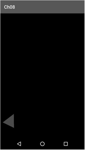
Figure 8-6. Our triangle cannon reacting to a touch event in the upper-right corner

Note that it doesn’t really matter whether we render a triangle at the cannon position or render a rectangle texture mapped to an image of a cannon—OpenGL ES doesn’t really care. We also have all the matrix operations in the present() method. The truth of the matter is that it is easier to keep track of OpenGL ES states this way, and we can use multiple view frustums in one present() call (for example, one view frustum setting up a world in meters, for rendering our world, and another view frustum setting up a world in pixels, for rendering UI elements). The impact on performance is not all that big, as described in Chapter 7, so it’s acceptable to do it this way most of the time. Just remember that you can optimize this if the need arises.

Vectors will be your best friends from now on. You can use them to specify virtually everything in your world. You will also be able to do some very basic physics with vectors. What’s a cannon good for if it can’t shoot, right?

Newton and Euler: Best Friends Forever

Our main concern is with the motion physics of so-called point masses. Motion physics describes the change in position, velocity, and acceleration of an object over time. Point mass means that all objects are approximated with an infinitesimally small point that has an associated mass. We do not have to deal with things like torque—the rotational velocity of an object around its center of mass—because that is a complex problem domain about which more than one complete book has been written. We will just look at these three properties of an object:

• Position: Represented as a vector in some space—in our case, a 2D space. Usually the position is given in meters.

• Velocity: The object’s change in position per second. Velocity is given as a 2D velocity vector, which is a combination of the unit-length direction vector in which the object is heading and the speed at which the object will move, given in meters per second (m/s). Note that the speed just governs the length of the velocity vector; if you normalize the velocity vector by the speed, you get a nice unit-length direction vector.

• Acceleration: The object’s change in velocity per second. We can represent this either as a scalar that only affects the speed of the velocity (the length of the velocity vector) or as a 2D vector so that we can have different acceleration in the x and y axes. Here, we’ll choose the latter, as it allows us to use things such as ballistics more easily. Acceleration is usually given in meters per second per second (m/s²). No, that’s not a typo—you change the velocity by some amount given in meters per second, each second.

When we know the properties of an object for a given point in time, we can integrate them to simulate the object’s path through the world over time. This may sound scary, but we already did this with Mr. Nom and our BobTest class. In those cases, we didn’t use acceleration; we simply set the velocity to a fixed vector. Here’s how we can integrate the acceleration, velocity, and position of an object in general:

Vector2 position = new Vector2();
Vector2 velocity = new Vector2();
Vector2 acceleration = new Vector2(0, -10);
while(simulationRuns) {
   float deltaTime = getDeltaTime();
   velocity.add(acceleration.x * deltaTime, acceleration.y * deltaTime);
   position.add(velocity.x * deltaTime, velocity.y * deltaTime);
}

This is called numerical Euler integration, and it is the most intuitive of the integration methods used in games. We start off with a position at (0,0), a velocity given as (0,0), and an acceleration of (0,–10), which means that the velocity will increase by 1 m/s on the y axis. There will be no movement on the x axis. Before we enter the integration loop, our object is standing still. Within the loop, we first update the velocity, based on the acceleration multiplied by the delta time, and then update the position, based on the velocity multiplied by the delta time. That’s all there is to the big, scary word integration.

Force and Mass

You might wonder where the acceleration comes from. That’s a good question with many answers. The acceleration of a car comes from its engine. The engine applies a force to the car that causes it to accelerate. But that’s not all. A car will also accelerate toward the center of the Earth because of gravity. The only thing that keeps it from falling through to the center of the Earth is the ground, which it can’t pass through. The ground cancels out this gravitational force. The general idea is this:

force = mass × acceleration

You can rearrange this to the following equation:

acceleration = force / mass

Force is given in the SI unit Newton. (Guess who came up with this.) If you specify acceleration as a vector, then you also have to specify force as a vector. A force can thus have a direction. For example, the gravitational force pulls downward in the direction (0,–1). The acceleration is also dependent on the mass of an object. The greater the mass of an object, the more force you need to apply in order to make it accelerate as fast as an object of less weight. This is a direct consequence of the preceding equations.

For simple games we can, however, ignore the mass and force and just work with the velocity and acceleration directly. The pseudocode in the preceding section sets the acceleration to (0,–10) m/s² (again, not a typo), which is roughly the acceleration of an object when it is falling toward the Earth, no matter its mass (ignoring things like air resistance). It’s true . . . ask Galileo!

Playing Around, Theoretically

We’ll use the preceding example to play with an object falling toward Earth. Let’s assume that we let the loop iterate ten times and that getDeltaTime() will always return 0.1 s. We’ll get the following positions and velocities for each iteration:

time=0.1, position=(0.0,-0.1), velocity=(0.0,-1.0)
time=0.2, position=(0.0,-0.3), velocity=(0.0,-2.0)
time=0.3, position=(0.0,-0.6), velocity=(0.0,-3.0)
time=0.4, position=(0.0,-1.0), velocity=(0.0,-4.0)
time=0.5, position=(0.0,-1.5), velocity=(0.0,-5.0)
time=0.6, position=(0.0,-2.1), velocity=(0.0,-6.0)
time=0.7, position=(0.0,-2.8), velocity=(0.0,-7.0)
time=0.8, position=(0.0,-3.6), velocity=(0.0,-8.0)
time=0.9, position=(0.0,-4.5), velocity=(0.0,-9.0)
time=1.0, position=(0.0,-5.5), velocity=(0.0,-10.0)

After 1 s, our object will fall 5.5 m and have a velocity of (0,–10) m/s, moving straight down to the core of the Earth (until it hits the ground, of course).

Our object will increase its downward speed without end, as we haven’t factored in air resistance. (As mentioned before, you can easily cheat your own system.) We can simply enforce a maximum velocity by checking the current velocity length, which equals the speed of the object.

All-knowing Wikipedia indicates that a human in free fall can have a maximum, or terminal, velocity of roughly 125 mph. Converting that to meters per second (125 × 1.6 × 1000 / 3600), we get 55.5 m/s. To make our simulation more realistic, we can modify the loop as follows:

while(simulationRuns) {
   float deltaTime = getDeltaTime();
   if(velocity.len() < 55.5)
      velocity.add(acceleration.x * deltaTime, acceleration.y * deltaTime);
   position.add(velocity.x * deltaTime, velocity.y * deltaTime);
}

As long as the speed of the object (the length of the velocity vector) is smaller than 55.5 m/s, we can increase the velocity by the acceleration. When we’ve reached the terminal velocity, we simply stop increasing it by the acceleration. This simple capping of velocities is a trick that is used heavily in many games.

We can add wind to the equation by adding another acceleration in the x direction, say (–1,0) m/s². For this, we add the gravitational acceleration to the wind acceleration before we add it to the velocity:

Vector2 gravity = new Vector2(0,-10);
Vector2 wind = new Vector2(-1,0);
while(simulationRuns) {
   float deltaTime = getDeltaTime();
   acceleration.set(gravity).add(wind);
   if(velocity.len() < 55.5)
      velocity.add(acceleration.x * deltaTime, acceleration.y * deltaTime);
   position.add(velocity.x * deltaTime, velocity.y * deltaTime);
}

We can also ignore acceleration altogether and let our objects have a fixed velocity. We did exactly this in the BobTest. We changed the velocity of each Bob only if he hit an edge, and we did so instantly.

Playing Around, Practically

The possibilities, even with this simple model, are endless. In this section, we’ll extend our little CannonTest from earlier in the chapter so that we can actually shoot a cannonball. Here’s what we want to do:

• As long as we drag our finger over the screen, the canon will follow it. That’s how we can specify the angle at which you’ll shoot the ball.

• As soon as we receive a touch-up event, we can fire a cannonball in the direction the cannon is pointing. The initial velocity of the cannonball will be a combination of the cannon’s direction and the speed the cannonball has from the start. The speed is equal to the distance between the cannon and the touch point. The further away we touch, the faster the cannonball will fly.

• The cannonball will fly as long as there’s no new touch-up event.

• We can double the size of the view frustum from (0,0) to (9.6, 6.4) so that we can see more of our world. Additionally, we can place the cannon at (0,0). Note that all units of the world are now given in meters.

• We can render the cannonball as a red rectangle of the size 0.2×0.2 m, or 20×20 cm—close enough to a real cannonball. The pirates among you may choose a more realistic size, of course.

Initially, the position of the cannonball will be (0,0)—the same as the cannon’s position. The velocity will also be (0,0). Since we apply gravity in each update, the cannonball will simply fall straight down.

Once a touch-up event is received, we set the ball’s position back to (0,0) and its initial velocity to (Math.cos(cannonAngle),Math.sin(cannonAngle)). This will ensure that the cannonball flies in the direction the cannon is pointing. Also, we set the speed simply by multiplying the velocity by the distance between the touch point and the cannon. The closer the touch point to the cannon, the more slowly the cannonball will fly.

Sounds easy enough, so now we can try implementing it. Copy over the code from the CannonTest.java file to a new file called CannonGravityTest.java. Rename the classes contained in that file to CannonGravityTest and CannonGravityScreen. Listing 8-3 shows the CannonGravityScreen class, with some comments added for clarity.

Listing 8-3. Excerpt from CannonGravityTest

class CannonGravityScreen extends Screen {
    float FRUSTUM_WIDTH = 2f;
    float FRUSTUM_HEIGHT = 2.5f;
    GLGraphics glGraphics = null;
    Vector2 cannonPos = new Vector2();
    float cannonAngle = 0;
    Vertices cannonVertices;
    Vertices ballVertices;
    Vector2 touchPos = new Vector2();
    Vector2 ballPos = new Vector2(0,0);
    Vector2 ballVelocity = new Vector2(0,0);            
    Vector2 gravity = new Vector2(0,-10);

Not a lot has changed. We simply doubled the size of the view frustum and reflected that by setting FRUSTUM_WIDTH and FRUSTUM_HEIGHT to 9.6 and 6.2, respectively. This means that we can see a rectangle of 9.2×6.2 m of the world. Since we also want to draw the cannonball, we add another set of vertices, which will hold the four vertices and six indices of the rectangle of the cannonball. The new members ballPos and ballVelocity store the position and velocity of the cannonball, and the member gravity is the gravitational acceleration, which will stay at a constant (0,–10) m/s² over the lifetime of our program.

public CannonGravityScreen(Game game) {
        super(game);
        glGraphics = ((GLGame) game).getGLGraphics();
        cannonVertices = new Vertices(glGraphics, 3, 0, false, false);
        cannonVertices.setVertices(new float[] { -0.5f, -0.5f,
                                            0.5f, 0.0f,
                                           -0.5f, 0.5f }, 0, 6);
        ballVertices = new Vertices(glGraphics, 4, 6, false, false);
        ballVertices.setVertices(new float[] { -0.1f, -0.1f,
                                                0.1f, -0.1f,
                                                0.1f,  0.1f,
                                               -0.1f,  0.1f }, 0, 8);
        ballVertices.setIndices(new short[] {0, 1, 2, 2, 3, 0}, 0, 6);
    }

In the constructor, we simply create the additional vertices for the rectangle of the cannonball. We define it in model space with the vertices (–0.1,–0.1), (0.1,–0.1), (0.1,0.1), and (–0.1,0.1). We use indexed drawing, and thus specify six vertices in this case.

@Override
public void update(float deltaTime) {
    List<TouchEvent> touchEvents = game.getInput().getTouchEvents();
    game.getInput().getKeyEvents();

    int len = touchEvents.size();
    for (int i = 0; i < len; i++) {
        TouchEvent event = touchEvents.get(i);

        touchPos.x = (event.x / (float) glGraphics.getWidth())
                * FRUSTUM_WIDTH;
        touchPos.y = (2.5f - event.y / (float) glGraphics.getHeight())
                * FRUSTUM_HEIGHT;
        cannonAngle = touchPos.sub(cannonPos).angle();

        if(event.type == TouchEvent.TOUCH_UP) {
            float radians = cannonAngle * Vector2.TO_RADIANS;
            float ballSpeed = touchPos.len();
            ballPos.set(cannonPos);
            ballVelocity.x = (float)Math.cos(radians) * ballSpeed;
            ballVelocity.y = (float)Math.sin(radians) * ballSpeed;
        }
    }

    ballVelocity.add(gravity.x * deltaTime, gravity.y * deltaTime);
    ballPos.add(ballVelocity.x * deltaTime, ballVelocity.y * deltaTime);
}

The update() method has changed only slightly. The calculation of the touch point in world coordinates and the angle of the cannon are still the same. The first addition is the if statement inside the event-processing loop. In case we get a touch-up event, we prepare the cannonball to be shot. We transform the cannon’s aiming angle to radians, as we’ll use Math.cos() and Math.sin() later on. Next, we calculate the distance between the cannon and the touch point. This will be the speed of the cannonball. We set the ball’s position to the cannon’s position. Finally, we calculate the initial velocity of the cannonball. We use sine and cosine, as discussed in the previous section, to construct a direction vector from the cannon’s angle. We multiply this direction vector by the cannonball’s speed to arrive at the final cannonball velocity. This is interesting, as the cannonball will have this velocity from the start. In the real world, the cannonball would, of course, accelerate from 0 m/s to whatever it could reach given air resistance, gravity, and the force applied to it by the cannon. We can cheat here, though, as that acceleration would happen in a very tiny time window (a couple hundred milliseconds). The last thing we do in the update() method is update the velocity of the cannonball and, based on that, adjust its position.

@Override
public void present(float deltaTime) {

    GL10 gl = glGraphics.getGL();
    gl.glViewport(0, 0, glGraphics.getWidth(), glGraphics.getHeight());
    gl.glClear(GL10.GL_COLOR_BUFFER_BIT);
    gl.glMatrixMode(GL10.GL_PROJECTION);
    gl.glLoadIdentity();
    gl.glOrthof(0, FRUSTUM_WIDTH, 0, FRUSTUM_HEIGHT, 1, -1);
    gl.glMatrixMode(GL10.GL_MODELVIEW);

    gl.glLoadIdentity();
    gl.glTranslatef(cannonPos.x, cannonPos.y, 0);
    gl.glRotatef(cannonAngle, 0, 0, 1);
    gl.glColor4f(1,1,1,1);
    cannonVertices.bind();
    cannonVertices.draw(GL10.GL_TRIANGLES, 0, 3);
    cannonVertices.unbind();

    gl.glLoadIdentity();
    gl.glTranslatef(ballPos.x, ballPos.y, 0);
    gl.glColor4f(1,0,0,1);
    ballVertices.bind();
    ballVertices.draw(GL10.GL_TRIANGLES, 0, 6);
    ballVertices.unbind();
}

In the present() method, we simply add the rendering of the cannonball rectangle. We do this after rendering the cannon’s triangle, which means that we have to “clean” the model-view matrix before we can render the rectangle. We do this with glLoadIdentity() and then use glTranslatef() to convert the cannonball’s rectangle from model space to world space at the ball’s current position.

    @Override
    public void pause() {

    }

    @Override
    public void resume() {

    }

    @Override
    public void dispose() {

    }        
}

If you run the example and touch the screen a couple of times, you’ll get a pretty good feel for how the cannonball will fly. Figure 8-7 shows the output (which is not all that impressive, since it is a still image).

Figure 8-7. A triangle cannon that shoots red rectangles. Impressive!

That’s enough physics for your purposes. With this simple model, we can simulate much more than cannonballs. Super Mario, for example, could be simulated in much the same way. If you have ever played Super Mario Brothers, you likely noticed that Mario takes a bit of time before he reaches his maximum velocity when running. This can be implemented with a very fast acceleration and velocity capping, as in the pseudocode of the last section. Jumping can be implemented in much the same way as shooting the cannonball. Mario’s current velocity would be adjusted by an initial jump velocity on the y axis (remember that you can add velocities like any other vectors). You would always apply a negative y acceleration (gravity), which makes him come back to the ground or fall into a pit after jumping. The velocity in the x direction is not influenced by what’s happening on the y axis. You can still press left and right to change the velocity of the x axis. The beauty of this simple model is that it allows you to implement very complex behavior with very little code. You can use this type of physics when you write your next game.

Simply shooting a cannonball is not a lot of fun. You want to be able to hit objects with the cannonball. For this, you need something called collision detection, which we’ll investigate in the next section.

Bounding Shapes

Once we have the final positions of our objects, we can perform collision testing, which boils down to testing for overlap. But what is it that overlaps? Each of our objects needs to have some mathematically defined form or shape that provides bounds for it. The correct term in this case is bounding shape. Figure 8-8 shows a few choices for bounding shapes.

Figure 8-8. Various bounding shapes around Bob

The properties of the three types of bounding shapes in Figure 8-8 are as follows:

• Triangle mesh: This bounds the object as tightly as possible by approximating its silhouette with a few triangles. It requires the most storage space, and it’s hard to construct and expensive to test against. It gives the most precise results, however. We won’t necessarily use the same triangles for rendering, but rather will simply store them for collision detection. The mesh can be stored as a list of vertices, with each subsequent set of three vertices forming a triangle. To conserve memory, we could also use indexed vertex lists.

• Axis-aligned bounding box: This bounds the object via a rectangle that is axis aligned, which means that the bottom and top edges are always aligned with the x axis, and the left and right edges are always aligned with the y axis. This is also fast to test against, but less precise than a triangle mesh. A bounding box is usually stored in the form of the position of its lower-left corner, plus its width and height. (In the case of 2D, this is also referred to as a bounding rectangle.)

• Bounding circle: This bounds the object with the smallest circle that can contain the object. It’s very fast to test against, but it is the least precise bounding shape. The circle is usually stored in the form of its center position and its radius.

Every object in our game gets a bounding shape that encloses it, in addition to its position, scale, and orientation. Of course, we need to adjust the bounding shape’s position, scale, and orientation according to the object’s position, scale, and orientation when we move the object; say, in a physics integration step.

Adjusting for position changes is easy: we simply move the bounding shape accordingly. In the case of the triangle mesh, move each vertex; in the case of the bounding rectangle, move the lower-left corner; and in the case of the bounding circle, move the center.

Scaling a bound shape is a little harder. We need to define the point around which we scale. This is usually the object’s position, which is often given as the center of the object. If we use this convention, then scaling is easy. For the triangle mesh, we scale the coordinates of each vertex; for the bounding rectangle, we scale its width, height, and lower-left corner position; and for the bounding circle, we scale its radius (the circle center is equal to the object’s center).

Rotating a bounding shape is dependent on the definition of a point around which to rotate. Using the convention just mentioned (where the object center is the rotation point), rotation also becomes easy. In the case of the triangle mesh, we simply rotate all vertices around the object’s center. In the case of the bounding circle, we do not have to do anything, as the radius will stay the same no matter how we rotate our object. The bounding rectangle is a little more involved. We need to construct all four corner points, rotate them, and then find the axis-aligned bounding rectangle that encloses those four points. Figure 8-9 shows the three bounding shapes after rotation.

Figure 8-9. Rotated bounding shapes, with the center of the object as the rotation point

While rotating a triangle mesh or a bounding circle is rather easy, the results for the axis-aligned bounding box are not all that satisfying. Notice that the bounding box of the original object fits tighter than its rotated version. There is a bounding box variant, called oriented bounding shape, that works better for rotation, but its disadvantage is that it’s harder to calculate. The bounding shapes covered so far are more than enough for our needs (and for most games out there). If you want to know more about oriented bounding shapes and really dive deep into collision detection, we recommend the book Real-Time Collision Detection by Christer Ericson.

Another question is: How do we create our bounding shapes for Bob in the first place?

Constructing Bounding Shapes

In the example shown in Figure 8-8, we simply constructed the bounding shapes by hand, based on Bob’s image. But what if Bob’s image is given in pixels, and your world operates in, say, meters? The solution to this problem involves normalization and model space. Imagine the two triangles we use for Bob in model space when we render him with OpenGL ES. The rectangle is centered at the origin in model space and has the same aspect ratio (width/height) as Bob’s texture image (that is, 32×32 pixels in the texture map, as compared to 2×2 m in model space). Now, we can apply Bob’s texture and figure out the locations of the points of the bounding shape in model space. Figure 8-10 shows how we can construct the bounding shapes around Bob in model space.

Figure 8-10. Bounding shapes around Bob in model space

This process may seem a little cumbersome, but the steps involved are not all that hard. The first thing we have to remember is how texture mapping works. We specify the texture coordinates for each vertex of Bob’s rectangle (which is composed of two triangles) in texture space. The upper-left corner of the texture image in texture space is at (0,0), and the lower-left corner is at (1,1), no matter the actual width and height of the image in pixels. To convert from the pixel space of our image to texture space, we can use this simple transformation:

u = x / imageWidth

v = y / imageHeight

where u and v are the texture coordinates of the pixel given by x and y in image space. The imageWidth and imageHeight are set to the image’s dimensions in pixels (32×32 in Bob’s case). Figure 8-11 shows how the center of Bob’s image maps to texture space.

Figure 8-11. Mapping a pixel from image space to texture space

The texture is applied to a rectangle that you define in model space. In the example in Figure 8-10, the upper-left corner is at (–1,1) and the lower-right corner is at (1,–1). We can use meters as the units in our world, so the rectangle has a width and height of 2 m. Additionally, we know that the upper-left corner has the texture coordinates (0,0) and the lower-right corner has the texture coordinates (1,1), so we can map the complete texture to Bob. This won’t always be the case, as you’ll see later in the texture atlas section.

Now we need a generic way to map from texture space to model space. We can make our life a little easier by constraining our mapping to only axis-aligned rectangles in texture space and model space. Assume that an axis-aligned rectangular region in texture space is mapped to an axis-aligned rectangle in model space. For the transformation, we need to know the width and height of the rectangle in model space and the width and height of the rectangle in texture space. In our Bob example, we have a 2×2 rectangle in model space and a 1×1 rectangle in texture space (since we map the complete texture to the rectangle). We also need to know the coordinates of the upper-left corner of each rectangle in its respective space. For the model space rectangle, that’s (–1,1); for the texture space rectangle, it’s (0,0) (again, since we map the complete texture, not just a portion). With this information, and the u and v coordinates of the pixel we want to map to model space, we can do the transformation with these two equations:

mx = (u – minU) / (tWidth) × mWidth + minX

my = (1 – ((v – minV) / (tHeight))× mHeight – minY

The variables u and v are the coordinates calculated in the previous transformation from pixel space to texture space. The variables minU and minV are the coordinates of the top-left corner of the region you map from texture space. The variables tWidth and tHeight are the width and height of your texture space region. The variables mWidth and mHeight are the width and height of your model space rectangle. The variables minX and minY are—you guessed it—the coordinates of the top-left corner of the rectangle in model space. Finally, mx and my are the transformed coordinates in model space.

These equations take the u and v coordinates, map them to the range 0 to 1, and then scale and position them in model space. Figure 8-12 shows a texel in texture space and how it is mapped to a rectangle in model space. On the sides, you see tWidth and tHeight and mWidth and mHeight. The top-left corner of each rectangle corresponds to (minU, minV) in texture space and (minX, minY) in model space.

Figure 8-12. Mapping from texture space to model space

Substituting the first two equations, we can go directly from pixel space to model space:

mx = ((x / imageWidth) – minU) / (tWidth) * mWidth + minX

my = (1 – (((y / imageHeight) – minV) / (tHeight)) * mHeight – minY

We can use these two equations to calculate the bounding shapes of our objects based on the image we map to their rectangles via texture mapping. In the case of the triangle mesh, this can get a little tedious; the bounding rectangle and bounding circle cases are a lot easier. Usually, you won’t need to take this hard route, but rather can create your textures so that the bounding rectangles at least have the same aspect ratio as the rectangle you render for the object via OpenGL ES. This way, you can construct the bounding rectangle from the object’s image dimension directly. The same is true for the bounding circle.

You should now know how to construct a nicely fitted bounding shape for your 2D objects. Define those bounding shape sizes manually when you create your graphical assets, and then define the units and sizes of your objects in the game world. You can then use these sizes in your code to collide objects.

Game Object Attributes

Bob just got fatter. In addition to the mesh we use for rendering (the rectangle mapping to Bob’s image texture), we now have a second data structure holding his bounds in some form. It is crucial to realize that, while we model the bounds after the mapped version of Bob in model space, the actual bounds are independent of the texture region to which you map Bob’s rectangle. Of course, we try to have a close match to the outline of Bob’s image in the texture when we create the bounding shape. It does not matter, however, whether the texture image is 32×32 pixels or 128×128 pixels. An object in our world thus has three attribute groups:

• Its position, orientation, scale, velocity, and acceleration: With these we can apply our physics model from the previous section. Of course, some objects might be static, and thus will only have position, orientation, and scale. Often, we can even leave out orientation and scale. The position of the object usually coincides with the origin in model space, as previously shown in Figure 8-10. This makes some calculations easier.

• Its bounding shape (usually constructed in model space around the object’s center): This coincides with its position and is aligned with its orientation and scale, as shown in Figure 8-10. This gives our object a boundary and defines its size in the world. We can make this shape as complex as we want. We could, for example, make it a composite of several bounding shapes.

• Its graphical representation: As shown in Figure 8-12, we still use two triangles to form a rectangle for Bob and then texture-map his image onto the rectangle. The rectangle is defined in model space, but does not necessarily equal the bounding shape, as shown in Figure 8-10. The graphical rectangle of Bob that we send to OpenGL ES is slightly larger than Bob’s bounding rectangle.

This separation of attributes allows us to apply our Model-View-Controller (MVC) pattern, as follows:

• On the model side, we have Bob’s physical attributes, composed of his position, scale, rotation, velocity, acceleration, and bounding shape. Bob’s position, scale, and orientation govern where his bounding shape is located in world space.

• The view simply takes Bob’s graphical representation (that is, the two texture-mapped triangles defined in model space) and renders it at its world space position according to Bob’s position, rotation, and scale. Here, we can use the OpenGL ES matrix operations as we did previously.

• The controller is responsible for updating Bob’s physical attributes according to user input (for example, a left button press could move him to the left) and according to physical forces, such as gravitational acceleration (like we applied to the cannonball in the previous section).

Of course, there’s some correspondence between Bob’s bounding shape and his graphical representation in the texture, as we base the bounding shape on that graphical representation. Our MVC pattern is thus not entirely clean, but we can live with that.

Broad-Phase and Narrow-Phase Collision Detection

We still don’t know how to check for collisions between our objects and their bounding shapes, however. There are two phases in collision detection:

• Broad phase: In this phase, we try to figure out which objects might potentially collide. Imagine having 100 objects that could collide with each other. We’d need to perform 100 × 100 / 2 overlap tests if we chose, naïvely, to test each object against the other objects. This naïve overlap testing approach is of O(n ²) asymptotic complexity, meaning it would take n ² steps to complete (it actually could be finished in half that many steps, but the asymptotic complexity leaves out any constants). In a good, non-brute-force broad phase, we can try to figure out which pairs of objects are actually in danger of colliding. Other pairs (for example, two objects that are too far apart for a collision to happen) will not be checked. We can reduce the computational load this way, as narrow-phase testing is usually pretty expensive.

• Narrow phase: Once we know which pairs of objects can potentially collide, we test whether they really collide or not by doing an overlap test on their bounding shapes.

We’ll discuss the narrow phase first and leave the broad phase for later, as the broad phase depends on some characteristics of our game, while the narrow phase can be implemented independently.

Narrow Phase

Once we are done with the broad phase, we have to check whether the bounding shapes of the potentially colliding objects overlap. As discussed earlier, we have a few options for bounding shapes. Triangle meshes are the most computationally expensive and cumbersome to create, but in most 2D games you don’t need them and can get away with using only bounding rectangles and bounding circles, so that’s what we’ll concentrate on here.

Circle Collision

Bounding circles are the cheapest way to check whether two objects collide, so let’s define a simple Circle class. Listing 8-4 shows the code.

Listing 8-4. Circle.java: A simple Circle class

package com.badlogic.androidgames.framework.math;

public class Circle {
    public final Vector2 center = new Vector2();
    public float radius;

    public Circle(float x, float y, float radius) {
        this.center.set(x,y);
        this.radius = radius;
    }
}

We store the center as a Vector2 and the radius as a simple float. How can we check whether two circles overlap? Take a look at Figure 8-13.

Figure 8-13. Two circles overlapping (left), and two circles not overlapping (right)

It’s very simple and computationally efficient. All we need to do is figure out the distance between the two centers. If the distance is greater than the sum of the two radii, then we know the two circles do not overlap. In code, this will appear as follows:

public boolean overlapCircles(Circle c1, Circle c2) {
    float distance = c1.center.dist(c2.center);
    return distance <= c1.radius + c2.radius;
}

First, we measure the distance between the two centers, and then check to see if the distance is smaller than or equal to the sum of the radii.

We have to take a square root in the Vector2.dist() method. This is unfortunate, as taking the square root is a costly operation. Can we make this faster? Yes, we can—all we need to do is reformulate our condition:

sqrt(dist.x × dist.x + dist.y × dist.y) <= radius1 + radius2

We can get rid of the square root by exponentiating both sides of the inequality, as follows:

dist.x × dist.x + dist.y × dist.y <= (radius1 + radius2) × (radius1 + radius2)

We trade the square root for another addition and multiplication on the right side. This is a lot better. Now we can create a Vector2.distSquared() function that will return the squared distance between two vectors:

public float distSquared(Vector2 other) {
    float distX = this.x - other.x;
    float distY = this.y - other.y;        
    return distX * distX + distY * distY;
}
public float distSquared(float x, float y) {
    float distX = this.x - x;
    float distY = this.y - y;
    return distX * distX + distY * distY;
}

We should also add a second distSquared() method that takes two floats (x and y) instead of a vector.

The overlapCircles() method then becomes the following:

public boolean overlapCircles(Circle c1, Circle c2) {
    float distance = c1.center.distSquared(c2.center);
    float radiusSum = c1.radius + c2.radius;
    return distance <= radiusSum * radiusSum;
}

Rectangle Collision

For rectangle collision, we first need a class that can represent a rectangle. As previously mentioned, we want a rectangle to be defined by its lower-left corner position, plus its width and height. Listing 8-5 does just that.

Listing 8-5. Rectangle.java, a Rectangle Class

package com.badlogic.androidgames.framework.math;

public class Rectangle {
    public final Vector2 lowerLeft;
    public float width, height;

    public Rectangle(float x, float y, float width, float height) {
        this.lowerLeft = new Vector2(x,y);
        this.width = width;
        this.height = height;
    }
}

We store the lower-left corner’s position in a Vector2 instance and the width and height in two floats. How can we check whether two rectangles overlap? Figure 8-14 should give you a hint.

Figure 8-14. Lots of overlapping and nonoverlapping rectangles

The first two cases, partial overlap (left) and nonoverlap (center), are easy. The case on the right is a surprise. A rectangle can, of course, be completely contained in another rectangle. This can happen in the case of circles, as well. However, our circle overlap test will return the correct result if one circle is contained in the other circle.

Checking for overlap in the rectangle case looks complex at first. However, we can create a very simple test if we use a little logic. Here’s the simplest method to check for overlap between two rectangles:

public Boolean overlapRectangles(Rectangle r1, Rectangle r2) {
    if(r1.lowerLeft.x < r2.lowerLeft.x + r2.width &&
       r1.lowerLeft.x + r1.width > r2.lowerLeft.x &&
       r1.lowerLeft.y < r2.lowerLeft.y + r2.height &&
       r1.lowerLeft.y + r1.height > r2.lowerLeft.y)
        return true;
    else                
        return false;
}

This looks a little confusing at first sight, so let’s go over each condition. The first condition states that the left edge of the first rectangle must be to the left of the right edge of the second rectangle. The next condition states that the right edge of the first rectangle must be to the right of the left edge of the second rectangle. The other two conditions state the same for the top and bottom edges of the rectangles. If all these conditions are met, then the two rectangles overlap. Double-check this with Figure 8-14. It also covers the containment case.

Circle/Rectangle Collision

Can we check for overlap between a circle and a rectangle? Yes, we can. However, this is a little more involved. Take a look at Figure 8-15.

Figure 8-15. Overlap-testing a circle and a rectangle by finding the point on/in the rectangle that is closest to the circle

The overall strategy to test for overlap between a circle and a rectangle goes like this:

• Find the x coordinate on or in the rectangle that is closest to the circle’s center. This coordinate can be a point either on the left or right edge of the rectangle, unless the circle center is contained in the rectangle, in which case the closest x coordinate is the circle center’s x coordinate.

• Find the y coordinate on or in the rectangle that is closest to the circle’s center. This coordinate can be a point either on the top or bottom edge of the rectangle, unless the circle center is contained in the rectangle, in which case the closest y coordinate is the circle center’s y coordinate.

• If the point composed of the closest x and y coordinates is within the circle, the circle and rectangle overlap.

While not depicted in Figure 8-15, this method also works for circles that completely contain the rectangle. Here’s the code:

public boolean overlapCircleRectangle(Circle c, Rectangle r) {
    float closestX = c.center.x;
    float closestY = c.center.y;

    if(c.center.x < r.lowerLeft.x) {
        closestX = r.lowerLeft.x;
    }
    else if(c.center.x > r.lowerLeft.x + r.width) {
        closestX = r.lowerLeft.x + r.width;
    }

    if(c.center.y < r.lowerLeft.y) {
        closestY = r.lowerLeft.y;
    }
    else if(c.center.y > r.lowerLeft.y + r.height) {
        closestY = r.lowerLeft.y + r.height;
    }

    return c.center.distSquared(closestX, closestY) < c.radius * c.radius;
}

The description looked a lot scarier than the implementation. We determine the closest point on the rectangle to the circle and then simply check whether the point lies inside the circle. If that’s the case, there is an overlap between the circle and the rectangle.

Note that we add an overloaded distSquared() method to Vector2 that takes two float arguments instead of another Vector2. We do the same for the dist() function.

Putting It All Together

Checking whether a point lies inside a circle or rectangle can also be useful. We can code up two more methods and put them in a class called OverlapTester, together with the other three methods we just defined. Listing 8-6 shows the code.

Listing 8-6. OverlapTester.java: Testing overlap between circles, rectangles, and points

package com.badlogic.androidgames.framework.math;                                                                                                                        

public class OverlapTester {
    public static boolean overlapCircles(Circle c1, Circle c2) {
        float distance = c1.center.distSquared(c2.center);
        float radiusSum = c1.radius + c2.radius;
        return distance <= radiusSum * radiusSum;
    }

    public static boolean overlapRectangles(Rectangle r1, Rectangle r2) {
        if(r1.lowerLeft.x < r2.lowerLeft.x + r2.width &&
           r1.lowerLeft.x + r1.width > r2.lowerLeft.x &&
           r1.lowerLeft.y < r2.lowerLeft.y + r2.height &&
           r1.lowerLeft.y + r1.height > r2.lowerLeft.y)
            return true;
        else                  
            return false;
    }

    public static boolean overlapCircleRectangle(Circle c, Rectangle r) {
        float closestX = c.center.x;
        float closestY = c.center.y;

        if(c.center.x < r.lowerLeft.x) {
            closestX = r.lowerLeft.x;
        }
        else if(c.center.x > r.lowerLeft.x + r.width) {
            closestX = r.lowerLeft.x + r.width;
        }

        if(c.center.y < r.lowerLeft.y) {
            closestY = r.lowerLeft.y;
        }
        else if(c.center.y > r.lowerLeft.y + r.height) {
            closestY = r.lowerLeft.y + r.height;
        }

        return c.center.distSquared(closestX, closestY) < c.radius * c.radius;
    }

    public static boolean pointInCircle(Circle c, Vector2 p) {
        return c.center.distSquared(p) < c.radius * c.radius;
    }

    public static boolean pointInCircle(Circle c, float x, float y) {
        return c.center.distSquared(x, y) < c.radius * c.radius;
    }

    public static boolean pointInRectangle(Rectangle r, Vector2 p) {
        return r.lowerLeft.x <= p.x && r.lowerLeft.x + r.width >= p.x &&
               r.lowerLeft.y <= p.y && r.lowerLeft.y + r.height >= p.y;
    }

    public static boolean pointInRectangle(Rectangle r, float x, float y) {
        return r.lowerLeft.x <= x && r.lowerLeft.x + r.width >= x &&
               r.lowerLeft.y <= y && r.lowerLeft.y + r.height >= y;
    }
}

Sweet! Now we have a fully functional 2D math library we can use for all our little physics models and for collision detection. We are ready to look at the broad phase in a little more detail.

Broad Phase

So, how can we achieve the magic that the broad phase promises? Consider Figure 8-16, which shows a typical Super Mario Brothers scene.

Figure 8-16. Super Mario and his enemies. Boxes around objects are their bounding rectangles; the big boxes make up a grid imposed on the world.

Can you guess what you can do to eliminate some collision checks? The grid in Figure 8-16 represents the cells with which we can partition our world. Each cell has the exact same size, and the whole world is covered in cells. Mario is currently in two of those cells, and the other objects with which Mario could potentially collide are in different cells. Thus, you don’t need to check for any collisions, as Mario is not in the same cells as any of the other objects in the scene. All we need to do is the following:

• Update all objects in the world based on our physics and controller step.

• Update the position of the bounding shape of each object according to the object’s position. We can, of course, also include the orientation and scale.

• Figure out in which cell or cells each object is contained, based on the bounding shape, and add these to the list of objects contained in those cells.

• Check for collisions, but only between object pairs that can collide (for example, Goombas don’t collide with other Goombas) and are in the same cell.

This is called a spatial hash grid broad phase, and it is very easy to implement. The first thing you have to define is the size of each cell. This is highly dependent on the scale and units you use for your game’s world.

An Elaborate Example

We’ll develop a spatial hash grid broad phase based on the previous cannonball example (located in the “Playing Around, Practically” section). We will completely rework it to incorporate everything covered in this section so far. In addition to the cannon and the cannonball, we also want to have targets. We make our life easy and just use 0.5×0.5-m squares as targets. These squares don’t move; they’re static. Our cannon is also static. The only thing that moves is the cannonball itself. We can generally categorize objects in our game world as static objects or dynamic objects. Let’s devise a class that represents such objects.

package com.badlogic.androidgames.framework;

import com.badlogic.androidgames.framework.math.Rectangle;
import com.badlogic.androidgames.framework.math.Vector2;

public class GameObject {
    public final Vector2 position;
    public final Rectangle bounds;

    public GameObject(float x, float y, float width, float height) {
        this.position = new Vector2(x,y);
        this.bounds = new Rectangle(x-width/2, y-height/2, width, height);
    }
}

package com.badlogic.androidgames.framework;

import com.badlogic.androidgames.framework.math.Vector2;

public class DynamicGameObject extends GameObject {
    public final Vector2 velocity;
    public final Vector2 accel;

    public DynamicGameObject(float x, float y, float width, float height) {
        super(x, y, width, height);
        velocity = new Vector2();
        accel = new Vector2();
    }
}

package com.badlogic.androidgames.gamedev2d;

public class Cannon extends GameObject {
    public float angle;

    public Cannon(float x, float y, float width, float height) {
        super(x, y, width, height);
        angle = 0;
    }
}

The Spatial Hash Grid

Our cannon will be bounded by a rectangle of 1×1 m, the cannonball will have a bounding rectangle of 0.2×0.2 m, and the targets will each have a bounding rectangle of 0.5×0.5 m. The bounding rectangles are centered on each object’s position to make our life a little easier.

When our cannon example starts up, we can simply place a number of targets at random positions. Here’s how we can set up the objects in our world:

Cannon cannon = new Cannon(0, 0, 1, 1);
DynamicGameObject ball = new DynamicGameObject(0, 0, 0.2f, 0.2f);
GameObject[] targets = new GameObject[NUM_TARGETS];
for(int i = 0; i < NUM_TARGETS; i++) {
    targets[i] = new GameObject((float)Math.random() * WORLD_WIDTH,
                                (float)Math.random() * WORLD_HEIGHT,
                                0.5f, 0.5f);  
}

The constants WORLD_WIDTH and WORLD_HEIGHT define the size of our game world. Everything should happen inside the rectangle bounded by (0,0) and (WORLD_WIDTH,WORLD_HEIGHT). Figure 8-17 shows a little mock-up of the game world so far.

Figure 8-17. A mock-up of the game world

Our world will look like this later on, but for now we can overlay a spatial hash grid. How big should the cells of the hash grid be? There’s no silver bullet, but a good heuristic is to have them five times bigger than the biggest object in the scene. In our example, the biggest object is the cannon, but we don’t collide anything with the cannon, so we can base the grid size on the next biggest objects in our scene, the targets. These are 0.5×0.5 m in size. A grid cell should thus have a size of 2.5×2.5 m. Figure 8-18 shows the grid overlaid onto our world.

Figure 8-18. Our cannon world overlaid with a spatial hash grid consisting of 12 cells

We have a fixed number of cells—in the case of the cannon world, 12. We give each cell a unique number, starting at the bottom-left cell, which gets the ID 0. Note that the top cells actually extend outside the world. This is not a problem; we simply need to make sure all our objects stay inside the boundaries of the world.

What we want to do is figure out to which cell(s) an object belongs. Ideally, we want to calculate the IDs of the cells in which the object is contained. This allows you to use the following simple data structure to store your cells:

List<GameObject>[] cells;

That’s right; we represent each cell as a list of GameObjects. The spatial hash grid itself is just composed of an array of lists of GameObjects.

Now we can figure out the IDs of the cells in which an object is contained. Figure 8-18 shows a couple of targets that span two cells. In fact, a small object can span up to four cells, and an object bigger than a grid cell can span more than four cells. We can make sure this never happens by choosing the grid cell size to be a multiple of the size of the biggest object in our game. This leaves us with the possibility of one object being contained in, at most, four cells.

To calculate the cell IDs for an object, we simply take the four corner points of the bounding rectangle and check which cell each corner point is in. Determining the cell that a point is in is easy—we just need to divide its coordinates by the cell width. Say you have a point at (.5,.8) and a cell size of 2.5×2.5 m: the point would be in the cell with ID 5, as in Figure 8-18.

We can divide each of the point’s coordinates by the cell size to get 2D integer coordinates, as follows:

cellX = floor(point.x / cellSize) = floor(.5 / 2.5) = 1

cellY = floor(point.y / cellSize) = floor(.8 / 2.5) = 1

And from these cell coordinates, we can easily get the cell ID:

cellId = cellX + cellY × cellsPerRow = 1 + 1 × 4 = 5

The constant cellsPerRow is simply the number of cells we need to cover our world with cells on the x axis:

cellsPerRow = ceil(worldWidth / cellSize) = ceil(9.6 / 2.5) = 4

We can calculate the number of cells needed per column like this:

cellsPerColumn = ceil(worldHeight / cellSize) = ceil(6.4 / 2.5) = 3

Based on this, we can implement the spatial hash grid rather easily. We set it up by giving it the world’s size and the desired cell size. We assume that all the action is happening in the positive quadrant of the world. This means that all the x and y coordinates of the points in the world will be positive. This is a constraint we can accept.

From the parameters, the spatial hash grid can figure out how many cells it needs (cellsPerRow × cellsPerColumn). We can also add a simple method to insert an object into the grid that will use the object’s boundaries to determine the cells in which it is contained. The object will then be added to each cell’s list of the objects that it contains. If one of the corner points of the bounding shape of the object is outside the grid, we can just ignore that corner point.

In each frame, we reinsert every object into the spatial hash grid after we update its position. However, there are objects in our cannon world that don’t move, so inserting them anew for each frame is very wasteful. We make a distinction between dynamic objects and static objects by storing two lists per cell. One list will be updated each frame and will hold only moving objects, and the other list will be static and will be modified only when a new static object is inserted.

Finally, we need a method that returns a list of objects in the cells of the object we’d like to have collide with other objects. All this method does is check which cells the object in question is in, retrieve the list of dynamic and static objects in those cells, and return the list to the caller. Of course, we have to make sure that we don’t return any duplicates, which can happen if an object is in multiple cells.

Listing 8-10 shows the code (well, most of it). The SpatialHashGrid.getCellIds() method will be discussed in a minute, as it is a little involved.

Listing 8-10. Excerpt from SpatialHashGrid.java: A spatial hash grid implementation

package com.badlogic.androidgames.framework;

import java.util.ArrayList;
import java.util.List;

import com.badlogic.androidgames.framework.GameObject;

public class SpatialHashGrid {
    List<GameObject>[] dynamicCells;
    List<GameObject>[] staticCells;
    int cellsPerRow;
    int cellsPerCol;
    float cellSize;
    int[] cellIds = new int[4];
    List<GameObject> foundObjects;

As discussed, we store two cell lists, one for dynamic objects and one for static objects. We also store the cells per row and column, so that we can later decide whether a point we check is inside or outside the world. The cell size also needs to be stored. The cellIds array is a working array that we can use to store the four cell IDs a GameObject is contained in temporarily. If it is contained in only one cell, then only the first element of the array will be set to the cell ID of the cell that contains the object entirely. If the object is contained in two cells, then the first two elements of that array will hold the cell ID, and so on. To indicate the number of cell IDs, we set all “empty” elements of the array to –1. The foundObjects list is also a working list, which we can return upon a call to getPotentialColliders(). Why do we keep those two members instead of instantiating a new array and list each time one is needed? Remember the garbage collector monster.

    @SuppressWarnings("unchecked")
    public SpatialHashGrid(float worldWidth, float worldHeight, float cellSize) {
        this.cellSize = cellSize;
        this.cellsPerRow = (int)Math.ceil(worldWidth / cellSize);
        this.cellsPerCol = (int)Math.ceil(worldHeight / cellSize);
        int numCells = cellsPerRow * cellsPerCol;
        dynamicCells = new List[numCells];
        staticCells = new List[numCells];
        for(int i = 0; i < numCells; i++) {
            dynamicCells[i] = new ArrayList<GameObject>(10);
            staticCells[i] = new ArrayList<GameObject>(10);
        }
        foundObjects = new ArrayList<GameObject>(10);
    }

The constructor of that class takes the world’s size and the desired cell size. From those arguments, we calculate how many cells are needed and instantiate the cell arrays and the lists holding the objects contained in each cell. Initialize the foundObjects list. All the ArrayList instances we create will have an initial capacity of ten GameObject instances. We do this to avoid memory allocations. The assumption is that it is unlikely that one single cell will contain more than ten GameObject instances. As long as that is true, the array lists don’t need to be resized.

public void insertStaticObject(GameObject obj) {
    int[] cellIds = getCellIds(obj);
    int i = 0;
    int cellId = -1;
    while(i <= 3 && (cellId = cellIds[i++]) != -1) {
        staticCells[cellId].add(obj);
    }
}

public void insertDynamicObject(GameObject obj) {
    int[] cellIds = getCellIds(obj);
    int i = 0;
    int cellId = -1;
    while(i <= 3 && (cellId = cellIds[i++]) != -1) {
        dynamicCells[cellId].add(obj);
    }
}

Next up are the methods insertStaticObject() and insertDynamicObject(). They calculate the IDs of the cells in which the object is contained via a call to getCellIds() and then insert the object into the appropriate list accordingly. The getCellIds() method will actually fill the cellIds member array.

public void removeObject(GameObject obj) {
    int[] cellIds = getCellIds(obj);
    int i = 0;
    int cellId = -1;
    while(i <= 3 && (cellId = cellIds[i++]) != -1) {
        dynamicCells[cellId].remove(obj);
        staticCells[cellId].remove(obj);
    }
}

We also have a removeObject() method, which we can use to figure out which cells the object is in and then delete it from the dynamic or static lists accordingly. This will be needed when a game object dies, for example.

    public void clearDynamicCells(GameObject obj) {
        int len = dynamicCells.length;
        for(int i = 0; i < len; i++) {
            dynamicCells[i].clear();
        }
    }  

The clearDynamicCells() method will be used to clear all dynamic cell lists. We need to call this each frame before we reinsert the dynamic objects, as discussed earlier.

public List<GameObject> getPotentialColliders(GameObject obj) {
    foundObjects.clear();
    int[] cellIds = getCellIds(obj);
    int i = 0;
    int cellId = -1;
    while(i <= 3 && (cellId = cellIds[i++]) != -1) {
        int len = dynamicCells [cellId].size();
        for(int j = 0; j < len; j++) {
            GameObject collider = dynamicCells[cellId].get(j);
            if(!foundObjects.contains(collider))
                foundObjects.add(collider);
        }

        len = staticCells[cellId].size();
        for(int j = 0; j < len; j++) {
            GameObject collider = staticCells[cellId].get(j);
            if(!foundObjects.contains(collider))
                foundObjects.add(collider);
        }
    }
    return foundObjects;
}

Finally, the getPotentialColliders() method takes an object and returns a list of neighboring objects that are contained in the same cells as that object. We use the working list foundObjects to store the list of found objects. Again, we do not want to instantiate a new list each time this method is called. All we need to do is figure out which cells the object passed to the method is in. We then simply add all the dynamic and static objects found in those cells to the foundObjects list and make sure that there are no duplicates. Using foundObjects.contains() to check for duplicates is, of course, suboptimal, but given that the number of found objects will never be large, it is acceptable to use it in this case. If we run into performance problems, then this is our number one candidate for optimization. Sadly, this isn’t trivial. We can use a Set, of course, but that allocates new objects internally each time we add an object to it. For now, we just leave it as it is, knowing that we can come back to it if anything goes wrong performance-wise.

The method left out is SpatialHashGrid.getCellIds(). Listing 8-11 shows its code. Don’t be afraid, it only looks menacing.

Listing 8-11. The Rest of SpatialHashGrid.java: Implementing getCellIds()

    public int[] getCellIds(GameObject obj) {
        int x1 = (int)Math.floor(obj.bounds.lowerLeft.x / cellSize);
        int y1 = (int)Math.floor(obj.bounds.lowerLeft.y / cellSize);
        int x2 = (int)Math.floor((obj.bounds.lowerLeft.x + obj.bounds.width) / cellSize);
        int y2 = (int)Math.floor((obj.bounds.lowerLeft.y + obj.bounds.height) / cellSize);

        if(x1 == x2 && y1 == y2) {
            if(x1 >= 0 && x1 < cellsPerRow && y1 >= 0 && y1 < cellsPerCol)
                cellIds[0] = x1 + y1 * cellsPerRow;
            else                
            cellIds[0] = -1;
            cellIds[1] = -1;
            cellIds[2] = -1;
            cellIds[3] = -1;
        }
        else if(x1 == x2) {
            int i = 0;
            if(x1 >= 0 && x1 < cellsPerRow) {
                if(y1 >= 0 && y1 < cellsPerCol)
                    cellIds[i++] = x1 + y1 * cellsPerRow;
                if(y2 >= 0 && y2 < cellsPerCol)
                    cellIds[i++] = x1 + y2 * cellsPerRow;
            }
            while(i <= 3) cellIds[i++] = -1;
        }
        else if(y1 == y2) {
            int i = 0;
            if(y1 >= 0 && y1 < cellsPerCol) {
                if(x1 >= 0 && x1 < cellsPerRow)
                    cellIds[i++] = x1 + y1 * cellsPerRow;
                if(x2 >= 0 && x2 < cellsPerRow)
                    cellIds[i++] = x2 + y1 * cellsPerRow;
            }
            while(i <= 3) cellIds[i++] = -1;   
        }
        else {
            int i = 0;
            int y1CellsPerRow = y1 * cellsPerRow;
            int y2CellsPerRow = y2 * cellsPerRow;
            if(x1 >= 0 && x1 < cellsPerRow && y1 >= 0 && y1 < cellsPerCol)
                cellIds[i++] = x1 + y1CellsPerRow;
            if(x2 >= 0 && x2 < cellsPerRow && y1 >= 0 && y1 < cellsPerCol)
                cellIds[i++] = x2 + y1CellsPerRow;
            if(x2 >= 0 && x2 < cellsPerRow && y2 >= 0 && y2 < cellsPerCol)
                cellIds[i++] = x2 + y2CellsPerRow;
            if(x1 >= 0 && x1 < cellsPerRow && y2 >= 0 && y2 < cellsPerCol)
                cellIds[i++] = x1 + y2CellsPerRow;
            while(i <= 3) cellIds[i++] = -1;
        }
        return cellIds;
    }
}

The first four lines of this method calculate the cell coordinates of the bottom-left and top-right corners of the object’s bounding rectangle. This calculation was discussed earlier. To understand the rest of this method, think about how an object can overlap grid cells. There are four possibilities:

• The object is contained in a single cell. The bottom-left and top-right corners of the bounding rectangle thus have the same cell coordinates.

• The object overlaps two cells horizontally. The bottom-left corner is in one cell, and the top-right corner is in the cell to the right.

• The object overlaps two cells vertically. The bottom-left corner is in one cell, and the top-right corner is in the cell above.

• The object overlaps four cells. The bottom-left corner is in one cell, the bottom-right corner is in the cell to the right, the top-right corner is in the cell above that, and the top-left corner is in the cell above the first cell.

All this method does is make a special case for each of these possibilities. The first if statement checks for the single-cell case, the second if statement checks for the horizontal double-cell case, the third if statement checks for the vertical double-cell case, and the else block handles the case of an object overlapping four grid cells. In each of the four blocks, we make sure that we only set the cell ID if the corresponding cell coordinates are within the world. And that’s all there is to this method.

Now, the method looks like it should take a lot of computational power. And indeed it does, but less than its size would suggest. The most common case will be the first one, and processing that is pretty cheap. Can you see opportunities to optimize this method further?

class CollisionScreen extends Screen {
    final int NUM_TARGETS = 20;
    final float WORLD_WIDTH = 9.6f;
    final float WORLD_HEIGHT = 4.8f;
    GLGraphics glGraphics;        
    Cannon cannon;
    DynamicGameObject ball;
    List<GameObject> targets;
    SpatialHashGrid grid;

    Vertices cannonVertices;
    Vertices ballVertices;
    Vertices targetVertices;
                                                                                                                  
    Vector2 touchPos = new Vector2();
    Vector2 gravity = new Vector2(0,-10);

    public CollisionScreen(Game game) {
        super(game);
        glGraphics = ((GLGame)game).getGLGraphics();

        cannon = new Cannon(0, 0, 1, 1);
        ball = new DynamicGameObject(0, 0, 0.2f, 0.2f);
        targets = new ArrayList<GameObject>(NUM_TARGETS);
        grid = new SpatialHashGrid(WORLD_WIDTH, WORLD_HEIGHT, 2.5f);
        for(int i = 0; i < NUM_TARGETS; i++) {
            GameObject target = new GameObject((float)Math.random() * WORLD_WIDTH,
                                               (float)Math.random() * WORLD_HEIGHT,
                                               0.5f, 0.5f);  
            grid.insertStaticObject(target);
            targets.add(target);
        }                        

        cannonVertices = new Vertices(glGraphics, 3, 0, false, false);
        cannonVertices.setVertices(new float[] { -0.5f, -0.5f,
                                                  0.5f, 0.0f,
                                                 -0.5f, 0.5f }, 0, 6);

        ballVertices = new Vertices(glGraphics, 4, 6, false, false);            
        ballVertices.setVertices(new float[] { -0.1f, -0.1f,
                                                0.1f, -0.1f,
                                                0.1f,  0.1f,
                                               -0.1f,  0.1f }, 0, 8);
        ballVertices.setIndices(new short[] {0, 1, 2, 2, 3, 0}, 0, 6);

        targetVertices = new Vertices(glGraphics, 4, 6, false, false);
        targetVertices.setVertices(new float[] { -0.25f, -0.25f,
                                                  0.25f, -0.25f,
                                                  0.25f,  0.25f,
                                                 -0.25f,  0.25f }, 0, 8);
        targetVertices.setIndices(new short[] {0, 1, 2, 2, 3, 0}, 0, 6);
    }

@Override
public void update(float deltaTime) {
    List<TouchEvent> touchEvents = game.getInput().getTouchEvents();
    game.getInput().getKeyEvents();

    int len = touchEvents.size();
    for (int i = 0; i < len; i++) {
        TouchEvent event = touchEvents.get(i);

        touchPos.x = (event.x / (float) glGraphics.getWidth()) * WORLD_WIDTH;
        touchPos.y = (1 - event.y / (float) glGraphics.getHeight()) * WORLD_HEIGHT;

        cannon.angle = touchPos.sub(cannon.position).angle();                      

        if(event.type == TouchEvent.TOUCH_UP) {
            float radians = cannon.angle * Vector2.TO_RADIANS;
            float ballSpeed = touchPos.len() * 2;
            ball.position.set(cannon.position);
            ball.velocity.x = (float)Math.cos(radians) * ballSpeed;
            ball.velocity.y = (float)Math.sin(radians) * ballSpeed;
            ball.bounds.lowerLeft.set(ball.position.x - 0.1f, ball.position.y - 0.1f);
        }
    }

    ball.velocity.add(gravity.x * deltaTime, gravity.y * deltaTime);
    ball.position.add(ball.velocity.x * deltaTime, ball.velocity.y * deltaTime);
    ball.bounds.lowerLeft.add(ball.velocity.x * deltaTime, ball.velocity.y * deltaTime);

    List<GameObject> colliders = grid.getPotentialColliders(ball);
    len = colliders.size();
    for(int i = 0; i < len; i++) {
        GameObject collider = colliders.get(i);
        if(OverlapTester.overlapRectangles(ball.bounds, collider.bounds)) {
            grid.removeObject(collider);
            targets.remove(collider);
        }
    }
}                                                                                                              

@Override
public void present(float deltaTime) {
    GL10 gl = glGraphics.getGL();
    gl.glViewport(0, 0, glGraphics.getWidth(), glGraphics.getHeight());
    gl.glClear(GL10.GL_COLOR_BUFFER_BIT);
    gl.glMatrixMode(GL10.GL_PROJECTION);
    gl.glLoadIdentity();
    gl.glOrthof(0, WORLD_WIDTH, 0, WORLD_HEIGHT, 1, -1);
    gl.glMatrixMode(GL10.GL_MODELVIEW);

    gl.glColor4f(0, 1, 0, 1);                                                                                                              
    targetVertices.bind();
    int len = targets.size();
    for(int i = 0; i < len; i++) {              
        GameObject target = targets.get(i);
        gl.glLoadIdentity();
        gl.glTranslatef(target.position.x, target.position.y, 0);
        targetVertices.draw(GL10.GL_TRIANGLES, 0, 6);
    }
    targetVertices.unbind();

    gl.glLoadIdentity();
    gl.glTranslatef(ball.position.x, ball.position.y, 0);
    gl.glColor4f(1,0,0,1);
    ballVertices.bind();
    ballVertices.draw(GL10.GL_TRIANGLES, 0, 6);
    ballVertices.unbind();  

    gl.glLoadIdentity();
    gl.glTranslatef(cannon.position.x, cannon.position.y, 0);
    gl.glRotatef(cannon.angle, 0, 0, 1);
    gl.glColor4f(1,1,1,1);
    cannonVertices.bind();
    cannonVertices.draw(GL10.GL_TRIANGLES, 0, 3);
    cannonVertices.unbind();
}

The Camera2D Class

Let’s put all this together into a single class. We want it to store the camera’s position, the standard frustum width and height, and the zoom factor. We also want a convenient method that sets the viewport (always use the whole screen) and projection matrix correctly. Additionally, we want a method that can translate touch coordinates to world coordinates. Listing 8-15 shows our new Camera2D class, with some comments.

Listing 8-15. Camera2D.java: Our shiny new camera class for 2D rendering

package com.badlogic.androidgames.framework.gl;

import javax.microedition.khronos.opengles.GL10;

import com.badlogic.androidgames.framework.impl.GLGraphics;
import com.badlogic.androidgames.framework.math.Vector2;

public class Camera2D {
    public final Vector2 position;
    public float zoom;
    public final float frustumWidth;
    public final float frustumHeight;
    final GLGraphics glGraphics;

As discussed, we store the camera’s position, frustum width and height, and zoom factor as members. The position and zoom factor are public, so we can easily manipulate them. We also need a reference to GLGraphics so that we can get the up-to-date width and height of the screen in pixels for transforming touch coordinates to world coordinates.

public Camera2D(GLGraphics glGraphics, float frustumWidth, float frustumHeight) {
    this.glGraphics = glGraphics;
    this.frustumWidth = frustumWidth;
    this.frustumHeight = frustumHeight;
    this.position = new Vector2(frustumWidth / 2, frustumHeight / 2);
    this.zoom = 1.0f;
}

In the constructor, we take a GLGraphics instance and the frustum’s width and height at zoom factor 1 as parameters. We store them and initialize the position of the camera to look at the center of the box bounded by (0,0,1) and (frustumWidth, frustumHeight,–1), as shown in Figure 8-19. The initial zoom factor is set to 1.

public void setViewportAndMatrices() {
    GL10 gl = glGraphics.getGL();
    gl.glViewport(0, 0, glGraphics.getWidth(), glGraphics.getHeight());
    gl.glMatrixMode(GL10.GL_PROJECTION);
    gl.glLoadIdentity();
    gl.glOrthof(position.x - frustumWidth * zoom / 2,
                position.x + frustumWidth * zoom / 2,
                position.y - frustumHeight * zoom / 2,
                position.y + frustumHeight * zoom / 2,
                1, -1);
    gl.glMatrixMode(GL10.GL_MODELVIEW);
    gl.glLoadIdentity();
}

The setViewportAndMatrices() method sets the viewport to span the whole screen and sets the projection matrix in accordance with your camera’s parameters, as discussed previously. At the end of the method, we tell OpenGL ES that all further matrix operations are targeting the model-view matrix and then load an identity matrix. We call this method each frame so that we can start from a clean slate—no more direct OpenGL ES calls to set up our viewport and projection matrix.

    public void touchToWorld(Vector2 touch) {
        touch.x = (touch.x / (float) glGraphics.getWidth()) * frustumWidth * zoom;
        touch.y = (1 - touch.y / (float) glGraphics.getHeight()) * frustumHeight * zoom;
        touch.add(position).sub(frustumWidth * zoom / 2, frustumHeight * zoom / 2);
    }
}

The touchToWorld() method takes a Vector2 instance containing touch coordinates and transforms the vector to world space. This is the same as was just discussed; the only difference is that we can use our fancy Vector2 class.

An Example

We’ll now use the Camera2D class in your cannon example. Copy the CollisionTest file and rename it Camera2DTest. Rename the GLGame class inside the file Camera2DTest, and rename the CollisionScreen to classCamera2DScreen. There are a few little changes we have to make to use our new Camera2D class.

The first thing we do is add a new member to the Camera2DScreen class:

Camera2D camera;

We initialize this member in the constructor, as follows:

camera = new Camera2D(glGraphics, WORLD_WIDTH, WORLD_HEIGHT);

We pass in our GLGraphics instance and the world’s width and height, which we previously used as the frustum’s width and height in our call to glOrthof(). All we need to do now is replace our direct OpenGL ES calls in the present() method, which looked like this:

gl.glViewport(0, 0, glGraphics.getWidth(), glGraphics.getHeight());
gl.glClear(GL10.GL_COLOR_BUFFER_BIT);
gl.glMatrixMode(GL10.GL_PROJECTION);
gl.glLoadIdentity();
gl.glOrthof(0, WORLD_WIDTH, 0, WORLD_HEIGHT, 1, -1);
gl.glMatrixMode(GL10.GL_MODELVIEW);

We replace them with this:

gl.glClear(GL10.GL_COLOR_BUFFER_BIT);
camera.setViewportAndMatrices();

We still have to clear the framebuffer, of course, but all the other direct OpenGL ES calls are nicely hidden inside the Camera2D.setViewportAndMatrices() method. If you run that code, you’ll see that nothing has changed. Everything works like before—all we did was make things a little nicer and more flexible.

We can also simplify the update() method of the test. Since we added the Camera2D.touchToWorld() method to the Camera2D class, we might as well use it. We can replace this snippet from the update() method:

touchPos.x = (event.x / (float) glGraphics.getWidth()) * WORLD_WIDTH;
touchPos.y = (1 - event.y / (float) glGraphics.getHeight()) * WORLD_HEIGHT;

with this:

camera.touchToWorld(touchPos.set(event.x, event.y));

Neat—now everything is nicely encapsulated. But it would be very boring if we didn’t use the features of your Camera2D class to their full extent. Here’s the plan: we want to have the camera look at the world in the “normal” way as long as the cannonball does not fly. That’s easy; we’re already doing that. We can determine whether the cannonball flies or not by checking whether the y coordinate of its position is less than or equal to zero. Since we always apply gravity to the cannonball, it will fall even if we don’t shoot it, so that’s a cheap way to check matters.

Our new addition will come into effect when the cannonball is flying (when the y coordinate is greater than zero). We want the camera to follow the cannonball. We can achieve this by simply setting the camera’s position to the cannonball’s position. That will always keep the cannonball in the center of the screen. We also want to try out our zooming functionality. Therefore, we can increase the zoom factor depending on the y coordinate of the cannonball: the further away from zero, the higher the zoom factor. If the cannonball has a higher y coordinate, this will make the camera zoom out. Here’s what we need to add at the end of the update() method in our test’s screen:

if(ball.position.y > 0) {
    camera.position.set(ball.position);
    camera.zoom = 1 + ball.position.y / WORLD_HEIGHT;
} else {
    camera.position.set(WORLD_WIDTH / 2, WORLD_HEIGHT / 2);
    camera.zoom = 1;
}

As long as the y coordinate of our ball is greater than zero, the camera will follow it and zoom out. Just add a value to the standard zoom factor of 1. That value is just the relation between the ball’s y position and the world’s height. If the ball’s y coordinate is at WORLD_HEIGHT, the zoom factor will be 2, so we’ll see more of our world. The way this is done can be really arbitrary; we can come up with any formula that we want here—there’s nothing magical about it. In case the ball’s position is less than or equal to zero, we show the world normally, as we did in the previous examples.

An Example

We add this texture atlas to our previous example to make it look more beautiful. Bob will be your target.

Copy the Camera2DTest and modify it a little. Place the copy in a file called TextureAtlasTest.java and rename the two classes contained in it accordingly (TextureAtlasTest and TextureAtlasScreen).

The first thing we do is add a new member to the TextureAtlasScreen:

Texture texture;

Instead of creating a Texture in the constructor, we create it in the resume() method. Remember that textures will get lost when our application comes back from a paused state, so we have to re-create them in the resume() method:

@Override
public void resume() {
    texture = new Texture(((GLGame)game), "atlas.png");
}

Put the image from Figure 8-23 in the assets/ folder of the project and name it atlas.png. (Of course, it doesn’t contain the gridlines shown in the figure.)

Next, we need to change the definitions of the vertices. We have one Vertices instance for each entity type (cannon, cannonball, and Bob); each instance holds a single rectangle of four vertices and six indices, making up three triangles. All we need to do is add texture coordinates to each of the vertices in accordance with the texture atlas. We also change the cannon from being represented as a triangle to being represented as a 1×0.5 m rectangle. Here’s what we use to replace the old vertex-creation code in the constructor:

cannonVertices = new Vertices(glGraphics, 4, 6, false, true);
cannonVertices.setVertices(new float[] { -0.5f, -0.25f, 0.0f, 0.5f,
                                          0.5f, -0.25f, 1.0f, 0.5f,
                                          0.5f,  0.25f, 1.0f, 0.0f,
                                         -0.5f,  0.25f, 0.0f, 0.0f },
                                         0, 16);
cannonVertices.setIndices(new short[] {0, 1, 2, 2, 3, 0}, 0, 6);

ballVertices = new Vertices(glGraphics, 4, 6, false, true);            
ballVertices.setVertices(new float[] { -0.1f, -0.1f, 0.0f, 0.75f,
                                        0.1f, -0.1f, 0.25f, 0.75f,
                                        0.1f,  0.1f, 0.25f, 0.5f,
                                       -0.1f,  0.1f, 0.0f, 0.5f },
                                        0, 16);
ballVertices.setIndices(new short[] {0, 1, 2, 2, 3, 0}, 0, 6);

targetVertices = new Vertices(glGraphics, 4, 6, false, true);
targetVertices.setVertices(new float[] { -0.25f, -0.25f, 0.5f, 1.0f,
                                          0.25f, -0.25f, 1.0f, 1.0f,
                                          0.25f,  0.25f, 1.0f, 0.5f,
                                         -0.25f,  0.25f, 0.5f, 0.5f },
                                         0, 16);
targetVertices.setIndices(new short[] {0, 1, 2, 2, 3, 0}, 0, 6);

Each of our meshes is now made up of four vertices, each having a 2D position and texture coordinates. We add six indices to the mesh, specifying the two triangles we want to render. The cannon is a little smaller on the y axis. It now has a size of 1×0.5 m instead of 1×1 m. This is also reflected in the construction of the Cannon object earlier in the constructor:

cannon = new Cannon(0, 0, 1, 0.5f);

Since we don’t do any collision detection with the cannon itself, it doesn’t really matter what size we set in that constructor; we just do it for consistency.

The last thing we need to change is our render method. Here it is in its full glory:

@Override
public void present(float deltaTime) {
    GL10 gl = glGraphics.getGL();
    gl.glClear(GL10.GL_COLOR_BUFFER_BIT);
    camera.setViewportAndMatrices();

    gl.glEnable(GL10.GL_BLEND);
    gl.glBlendFunc(GL10.GL_SRC_ALPHA, GL10.GL_ONE_MINUS_SRC_ALPHA);
    gl.glEnable(GL10.GL_TEXTURE_2D);
    texture.bind();

    targetVertices.bind();
    int len = targets.size();
    for(int i = 0; i < len; i++) {              
        GameObject target = targets.get(i);
        gl.glLoadIdentity();
        gl.glTranslatef(target.position.x, target.position.y, 0);
        targetVertices.draw(GL10.GL_TRIANGLES, 0, 6);
    }
    targetVertices.unbind();

    gl.glLoadIdentity();
    gl.glTranslatef(ball.position.x, ball.position.y, 0);
    ballVertices.bind();
    ballVertices.draw(GL10.GL_TRIANGLES, 0, 6);
    ballVertices.unbind();  

    gl.glLoadIdentity();
    gl.glTranslatef(cannon.position.x, cannon.position.y, 0);
    gl.glRotatef(cannon.angle, 0, 0, 1);            
    cannonVertices.bind();
    cannonVertices.draw(GL10.GL_TRIANGLES, 0, 6);
    cannonVertices.unbind();
}

Here, we enable blending, set a proper blending function, enable texturing, and bind our atlas texture. We also slightly adapt the cannonVertices.draw() call, which now renders two triangles instead of one. That’s all there is to it. Figure 8-24 shows the results of our face-lifting operation.

Figure 8-24. Beautifying the cannon example with a texture atlas

There are a few more things you need to know about texture atlases:

• When you use GL_LINEAR as the minification and/or magnification filter, there might be artifacts when two images within the atlas are touching each other. This is due to the texture mapper actually fetching the four nearest texels from a texture for a pixel on the screen. When it does that for the border of an image, it also fetches texels from the neighboring image in the atlas. You can eliminate this problem by introducing an empty border of 2 pixels between your images. Even better, you can duplicate the border pixel of each image. The first solution is easier—just make sure your texture size stays a power of two.

• There’s no need to lay out all the images in the atlas in a fixed grid. You could put arbitrarily sized images in the atlas as tightly as possible. All you need to know is where an image starts and ends in the atlas so that you can calculate proper texture coordinates for it. Packing arbitrarily sized images is a nontrivial problem, however. There are a couple of tools on the Web that can help you with creating a texture atlas; just do a search and you’ll be hit with a plethora of options.

• Often you cannot group all the images of your game into a single texture atlas. Remember that there’s a maximum texture size that varies from device to device. You can safely assume that all devices support a texture size of 512×512 pixels (or even 1024×1024). So, you can just have multiple texture atlases. You should try to group into one atlas objects that will be seen on the screen together, though—say, all the objects of level 1 in one atlas, all the objects of level 2 in another, all the UI elements in another, and so on. Think about the logical grouping before finalizing your art assets.

• Remember how we drew numbers dynamically in Mr. Nom? We used a texture atlas for that. In fact, we can perform all dynamic text rendering via a texture atlas. Just put all the characters you need for your game into an atlas and render them on demand by mapping a rectangle to the appropriate characters in the atlas. There are tools you can find on the Web that will generate a bitmap font for you. For purposes of the upcoming chapters, we stick to the approach used in Mr. Nom: static text will be prerendered as a whole, and only dynamic text (for example, numbers in high scores) will be rendered via an atlas.

You might have noticed that the Bobs disappear before they are graphically hit by the cannonball. This is because our bounding shapes are a little too big. We have some white space around both Bob and the cannonball. What’s the solution? Just make the bounding shapes a little smaller. You should get a feel for this, so manipulate the source until the collision feels right. You will often find such fine-tuning “opportunities” while developing a game. Fine-tuning is probably one of the most crucial parts of game development, aside from good level design. Getting things to feel right can be hard, but it is highly satisfactory once you have achieved the level of perfection found in Super Mario Brothers. Sadly, this is nothing that can be taught, as it is dependent on the look and feel of your game. Consider it the magic sauce that sets good and bad games apart.

The TextureRegion Class

Since we’ve worked with texture regions already, it should be straightforward to figure out what we need. We know how to convert from pixel coordinates to texture coordinates. We want to have a class where we can specify pixel coordinates of an image in a texture atlas, which then stores the corresponding texture coordinates of the atlas region for further processing (for example, when we want to render a sprite). Without further ado, Listing 8-16 shows our TextureRegion class.

Listing 8-16. TextureRegion.java: Converting pixel coordinates to texture coordinates

package com.badlogic.androidgames.framework.gl;

public class TextureRegion {    
    public final float u1, v1;
    public final float u2, v2;
    public final Texture texture;

    public TextureRegion(Texture texture, float x, float y, float width, float height) {
        this.u1 = x / texture.width;
        this.v1 = y / texture.height;
        this.u2 = this.u1 + width / texture.width;
        this.v2 = this.v1 + height / texture.height;        
        this.texture = texture;
    }
}

The TextureRegion stores the texture coordinates of the top-left corner (u1,v1) and bottom-right corner (u2,v2) of the region. The constructor takes a Texture and the top-left corner, as well as the width and height of the region, in pixel coordinates. To construct a texture region for the cannon, we could do this:

TextureRegion cannonRegion = new TextureRegion(texture, 0, 0, 64, 32);

Similarly, we could construct a region for Bob:

TextureRegion bobRegion = new TextureRegion(texture, 32, 32, 32, 32);

And so on and so forth. We can use this in the example code that we’ve already created, and use the TextureRegion.u1, v1, u2, and v2 members for specifying the texture coordinates of the vertices of our rectangles. But we won’t need to do that, since we want to get rid of these tedious definitions altogether. That’s what we can use the sprite batcher for.

The SpriteBatcher Class

As already discussed , a sprite can be easily defined by its position, size, and texture region (and, optionally, its rotation and scale). It is simply a graphical rectangle in our world space. To make things easier, we stick to the convention of having the position be the center of the sprite and having the rectangle be constructed around that center. Now we can have a Sprite class and use it like this:

Sprite bobSprite = new Sprite(20, 20, 0.5f, 0.5f, bobRegion);

That would construct a new sprite, with its center at (20,20) in the world, extending 0.25 m to each side, and using the bobRegion TextureRegion. But we could do this instead:

spriteBatcher.drawSprite(bob.x, bob.y, BOB_WIDTH, BOB_HEIGHT, bobRegion);

Now, that looks a lot better. We don’t need to construct yet another object to represent the graphical side of your object. Instead, we draw an instance of Bob on demand. We could also have an overloaded method:

spriteBatcher.drawSprite(cannon.x, cannon.y, CANNON_WIDTH, CANNON_HEIGHT, cannon.angle, cannonRegion);

That would draw the cannon, rotated by its angle. So, how can we implement the sprite batcher? Where are the Vertices instances? Let’s think about how the batcher could work.

What is batching anyway? In the graphics community, batching is defined as collapsing multiple draw calls into a single draw call. This makes the GPU happy, as discussed in Chapter 7. A sprite batcher offers one way to make this happen. Here’s how:

• The batcher has a buffer that is empty initially (or becomes empty after we signal it to be cleared). That buffer will hold vertices. It will be a simple float array, in our case.

• Each time we call the SpriteBatcher.drawSprite() method, we add four vertices to the buffer based on the position, size, orientation, and texture region that were specified as arguments. This also means that we have to rotate and translate the vertex positions manually, without the help of OpenGL ES. Fear not, though, as the code of your Vector2 class will come in handy here. This is the key to eliminating all the draw calls.

• Once we have specified all the sprites we want to render, we tell the sprite batcher to submit the vertices for all the rectangles of the sprites to the GPU in one go and then call the actual OpenGL ES drawing method to render all the rectangles. For this, we can transfer the contents of the float array to a Vertices instance and use it to render the rectangles.

The usual usage pattern of a sprite batcher looks like this:

batcher.beginBatch(texture);
// call batcher.drawSprite() as often as needed,
// referencing regions in the texture
batcher.endBatch();

The call to SpriteBatcher.beginBatch() tells the batcher two things: it should clear its buffer, and it should use the texture we pass in. We will bind the texture within this method for convenience.

Next, we render as many sprites that reference regions within this texture as we need. This will fill the buffer, adding four vertices per sprite.

The call to SpriteBatcher.endBatch() signals to the sprite batcher that we are done rendering the batch of sprites and that it should now upload the vertices to the GPU for actual rendering. We are going to use indexed rendering with a Vertices instance, so we also need to specify the indices, in addition to the vertices, in the float array buffer. However, since we are always rendering rectangles, we can generate the indices once beforehand in the constructor of the SpriteBatcher. For this, we need to know how many sprites the batcher can draw per batch. By putting a hard limit on the number of sprites that can be rendered per batch, we don’t need to grow any arrays for other buffers; we can just allocate these arrays and buffers one time in the constructor.

The general mechanics are rather simple. The SpriteBatcher.drawSprite() method may seem like a mystery, but it’s not a big problem (if we leave out rotation and scaling for a moment). All we need to do is calculate the vertex positions and texture coordinates, as defined by the parameters. We have done this manually already in previous examples—for instance, when we defined the rectangles for the cannon, the cannonball, and Bob. We can do more or less the same thing in the SpriteBatcher.drawSprite() method, only automatically, based on the parameters of the method. So let’s check out SpriteBatcher. Listing 8-17 shows the code.

Listing 8-17. Excerpt from SpriteBatcher.java, Without Rotation and Scaling

package com.badlogic.androidgames.framework.gl;

import com.badlogic.androidgames.framework.impl.GLGraphics;
import com.badlogic.androidgames.framework.math.Vector2;

public class SpriteBatcher {
    final float[] verticesBuffer;
    int bufferIndex;
    Vertices vertices;
    int numSprites;    

We look at the members first. The member verticesBuffer is the temporary float array in which we store the vertices of the sprites of the current batch. The member bufferIndex indicates where in the float array we should start to write the next vertices. The member vertices is the Vertices instance used to render the batch. It also stores the indices that we’ll define in a minute. The member numSprites holds the number drawn so far in the current batch.

public SpriteBatcher(GLGraphics glGraphics, int maxSprites) {
    this.verticesBuffer = new float[maxSprites*4*4];

    this.vertices = new Vertices(glGraphics, maxSprites*4, maxSprites*6, false, true);

    this.bufferIndex = 0;
    this.numSprites = 0;

    short[] indices = new short[maxSprites*6];
    int len = indices.length;
    short j = 0;
    for (int i = 0; i < len; i += 6, j += 4) {
            indices[i + 0] = (short)(j + 0);
            indices[i + 1] = (short)(j + 1);
            indices[i + 2] = (short)(j + 2);
            indices[i + 3] = (short)(j + 2);
            indices[i + 4] = (short)(j + 3);
            indices[i + 5] = (short)(j + 0);
    }
    vertices.setIndices(indices, 0, indices.length);
}

Moving to the constructor, we have two arguments: the GLGraphics instance we need for creating the Vertices instance and the maximum number of sprites the batcher should be able to render in one batch. The first thing we do in the constructor is create the float array. We have four vertices per sprite, and each vertex takes up four floats (two for the x and y coordinates and another two for the texture coordinates). We can have maxSprites sprites maximally, so that’s 4 × 4 × maxSprites floats that we need for the buffer.

Next, we create the vertices. We need it to store maxSprites × 4 vertices and maxSprites × 6 indices. We then initialize the bufferIndex and numSprites members to zero. We need to do this only once, as the indices will never change. The first sprite in a batch will always have the indices 0, 1, 2, 2, 3, 0; the next sprite will have 4, 5, 6, 6, 7, 4; and so on. We can precompute these and store them in the Vertices instance. This way, we only need to set them once, instead of once for each sprite.

public void beginBatch(Texture texture) {
    texture.bind();
    numSprites = 0;
    bufferIndex = 0;
}

Next up is the beginBatch() method. It binds the texture and resets the numSprites and bufferIndex members so that the first sprite’s vertices will get inserted at the front of the verticesBuffer float array.

public void endBatch() {
    vertices.setVertices(verticesBuffer, 0, bufferIndex);
    vertices.bind();
    vertices.draw(GL10.GL_TRIANGLES, 0, numSprites * 6);
    vertices.unbind();
}

The next method is endBatch(); we’ll call it to finalize and draw the current batch. It first transfers the vertices defined for this batch from the float array to the Vertices instance. All that’s left is binding the Vertices instance, drawing numSprites × 2 triangles, and unbinding the Vertices instance again. Since we use indexed rendering, we specify the number of indices to use—which is six indices per sprite, times numSprites. That’s all there is to rendering.

    public void drawSprite(float x, float y, float width, float height, TextureRegion region) {
        float halfWidth = width / 2;
        float halfHeight = height / 2;
        float x1 = x - halfWidth;
        float y1 = y - halfHeight;
        float x2 = x + halfWidth;
    float y2 = y + halfHeight;

    verticesBuffer[bufferIndex++] = x1;
    verticesBuffer[bufferIndex++] = y1;
    verticesBuffer[bufferIndex++] = region.u1;
    verticesBuffer[bufferIndex++] = region.v2;

    verticesBuffer[bufferIndex++] = x2;
    verticesBuffer[bufferIndex++] = y1;
    verticesBuffer[bufferIndex++] = region.u2;
    verticesBuffer[bufferIndex++] = region.v2;

    verticesBuffer[bufferIndex++] = x2;
    verticesBuffer[bufferIndex++] = y2;
    verticesBuffer[bufferIndex++] = region.u2;
    verticesBuffer[bufferIndex++] = region.v1;

    verticesBuffer[bufferIndex++] = x1;
    verticesBuffer[bufferIndex++] = y2;
    verticesBuffer[bufferIndex++] = region.u1;
    verticesBuffer[bufferIndex++] = region.v1;

    numSprites++;
}

The next method, drawSprite(), is the workhorse of the SpriteBatcher class. It takes the x and y coordinates of the center of the sprite, its width and height, and the texture region to which it maps. The method’s responsibility is to add four vertices to the float array starting at the current bufferIndex. These four vertices form a texture-mapped rectangle. We calculate the position of the bottom-left corner (x1,y1) and the top-right corner (x2,y2) and use these four variables to construct the vertices together with the texture coordinates from the TextureRegion. The vertices are added in counterclockwise order, starting at the bottom-left vertex. Once they are added to the float array, we increment the numSprites counter and wait for another sprite to be added or for the batch to be finalized.

And that is all there is to do. We just eliminated a lot of drawing methods simply by buffering pre-transformed vertices in a float array and rendering them in one go. That will increase our 2D sprite-rendering performance considerably as compared to the method we were using before. Fewer OpenGL ES state changes and fewer drawing calls make the GPU happy.

There’s one more thing we need to implement: a SpriteBatcher.drawSprite() method that can draw a rotated sprite. All we need to do is construct the four corner vertices without adding the position, rotate them around the origin, add the position of the sprite so that the vertices are placed in the world space, and then proceed as in the previous drawing method. We could use Vector2.rotate() for this, but that would introduce additional function-call overhead. We therefore reproduce the code in Vector2.rotate() and optimize where possible. The final method of the SpriteBatcher class looks like Listing 8-18.

Listing 8-18. The rest of SpriteBatcher.java: A method to draw rotated sprites

    public void drawSprite(float x, float y, float width, float height, float angle, TextureRegion region) {
        float halfWidth = width / 2;
        float halfHeight = height / 2;

        float rad = angle * Vector2.TO_RADIANS;
        float cos = (float)Math.cos(rad);
        float sin = (float)Math.sin(rad);

        float x1 = -halfWidth * cos - (-halfHeight) * sin;
        float y1 = -halfWidth * sin + (-halfHeight) * cos;
        float x2 = halfWidth * cos - (-halfHeight) * sin;
        float y2 = halfWidth * sin + (-halfHeight) * cos;
        float x3 = halfWidth * cos - halfHeight * sin;
        float y3 = halfWidth * sin + halfHeight * cos;
        float x4 = -halfWidth * cos - halfHeight * sin;
        float y4 = -halfWidth * sin + halfHeight * cos;

        x1 += x;
        y1 += y;
        x2 += x;
        y2 += y;
        x3 += x;
        y3 += y;
        x4 += x;
        y4 += y;

        verticesBuffer[bufferIndex++] = x1;
        verticesBuffer[bufferIndex++] = y1;
        verticesBuffer[bufferIndex++] = region.u1;
        verticesBuffer[bufferIndex++] = region.v2;

        verticesBuffer[bufferIndex++] = x2;
        verticesBuffer[bufferIndex++] = y2;
        verticesBuffer[bufferIndex++] = region.u2;
        verticesBuffer[bufferIndex++] = region.v2;

        verticesBuffer[bufferIndex++] = x3;
        verticesBuffer[bufferIndex++] = y3;
        verticesBuffer[bufferIndex++] = region.u2;
        verticesBuffer[bufferIndex++] = region.v1;

        verticesBuffer[bufferIndex++] = x4;
        verticesBuffer[bufferIndex++] = y4;
        verticesBuffer[bufferIndex++] = region.u1;
        verticesBuffer[bufferIndex++] = region.v1;

        numSprites++;
    }
}

We do the same thing as in the simpler drawing method, except that we construct all four corner points instead of just the two opposite ones. This is needed for the rotation. The rest is the same as before.

What about scaling? We do not explicitly need another method, since scaling a sprite only requires scaling its width and height. We can do that outside of the two drawing methods, so there’s no need to have another bunch of methods for the scaled drawing of sprites.

And that’s the big secret behind lightning-fast sprite rendering with OpenGL ES.

TextureRegion cannonRegion;
TextureRegion ballRegion;
TextureRegion bobRegion;
SpriteBatcher batcher;

batcher = new SpriteBatcher(glGraphics, 100);

@Override
public void resume() {
    texture = new Texture(((GLGame)game), "atlas.png");
    cannonRegion = new TextureRegion(texture, 0, 0, 64, 32);
    ballRegion = new TextureRegion(texture, 0, 32, 16, 16);
    bobRegion = new TextureRegion(texture, 32, 32, 32, 32);
}

@Override
public void present(float deltaTime) {
    GL10 gl = glGraphics.getGL();
    gl.glClear(GL10.GL_COLOR_BUFFER_BIT);
    camera.setViewportAndMatrices();

    gl.glEnable(GL10.GL_BLEND);
    gl.glBlendFunc(GL10.GL_SRC_ALPHA, GL10.GL_ONE_MINUS_SRC_ALPHA);
    gl.glEnable(GL10.GL_TEXTURE_2D);

    batcher.beginBatch(texture);

    int len = targets.size();
    for(int i = 0; i < len; i++) {              
        GameObject target = targets.get(i);
        batcher.drawSprite(target.position.x, target.position.y, 0.5f, 0.5f, bobRegion);
    }

    batcher.drawSprite(ball.position.x, ball.position.y, 0.2f, 0.2f, ballRegion);
    batcher.drawSprite(cannon.position.x, cannon.position.y, 1, 0.5f, cannon.angle, cannonRegion);            
    batcher.endBatch();
}

The Animation Class

Let us define the requirements for an Animation class, which stores the data for a single animation, such as the walk animation in Figure 8-25:

• An Animation holds a number of TextureRegions, which store the location of each keyframe in the texture atlas. The order of the TextureRegions is the same as that used for playing back the animation.

• The Animation also stores the frame duration, which has to pass before we switch to the next frame.

• The Animation should provide us with a method to which we pass the time we’ve been in the state that the Animation represents (for example, walking left), and that will return the appropriate TextureRegion. The method should take into consideration whether we want the Animation to loop or to stay at the last frame when the end is reached.

This last bullet point is important because it allows us to store a single Animation instance to be used by multiple objects in our world. An object just keeps track of its current state; that is, whether it is walking, shooting, or jumping, and how long it has been in that state. When we render this object, we use the state to select the animation we want to play back and the state time to get the correct TextureRegion from the Animation. Listing 8-19 shows the code of our new Animation class.

Listing 8-19. Animation.java: A simple animation class

package com.badlogic.androidgames.framework.gl;

public class Animation {
    public static final int ANIMATION_LOOPING = 0;
    public static final int ANIMATION_NONLOOPING = 1;

    final TextureRegion[] keyFrames;
    final float frameDuration;

    public Animation(float frameDuration, TextureRegion ... keyFrames) {
        this.frameDuration = frameDuration;
        this.keyFrames = keyFrames;
    }

    public TextureRegion getKeyFrame(float stateTime, int mode) {
        int frameNumber = (int)(stateTime / frameDuration);

        if(mode == ANIMATION_NONLOOPING) {
            frameNumber = Math.min(keyFrames.length-1, frameNumber);            
        } else {
            frameNumber = frameNumber % keyFrames.length;
        }
        return keyFrames[frameNumber];
    }
}

First, we define two constants to be used with the getKeyFrame() method. The first one says the animation should be looping, and the second one says that it should stop at the last frame.

Next, we define two members: an array holding the TextureRegions and a float storing the frame duration.

We pass the frame duration and the TextureRegions that hold the keyframes to the constructor, which simply stores them. We can make a defensive copy of the keyFrames array, but that would allocate a new object, which would make the garbage collector a little mad.

The interesting piece is the getKeyFrame() method. We pass in the time that the object has been in the state that the animation represents, as well as the mode, either Animation.ANIMATION_LOOPING or Animation.NON_LOOPING. We calculate how many frames have already been played for the given state based on the stateTime. If the animation shouldn’t be looping, we simply clamp the frameNumber to the last element in the TextureRegion array. Otherwise, we take the modulus, which will automatically create the looping effect we desire (for example, 4 % 3 = 1). All that’s left is returning the proper TextureRegion.

An Example

This section shows how to create an example called AnimationTest with a corresponding screen called AnimationScreen. As always, only the screen itself will be discussed.

We want to render a number of cavemen, all walking to the left. Our world will be the same size as our view frustum, which has the size 4.8×3.2 m. (This is arbitrary; we could use any size.) A caveman is a DynamicGameObject with a size of 1×1 m. We will derive from DynamicGameObject and create a new class called Caveman, which will store an additional member that keeps track of how long the caveman has been walking. Each caveman will move 0.5 m/s, either to the left or to the right. Add an update() method to the Caveman class to update the caveman’s position based on the delta time and his velocity. If a caveman reaches the left or right edge of the world, we set him to the other side of the world. We use the image in Figure 8-25 and create TextureRegion instances and an Animation instance accordingly. For rendering, we use a Camera2D instance and a SpriteBatcher because they are fancy. Listing 8-20 shows the code of the Caveman class.

Listing 8-20. Excerpt from AnimationTest.java: Showing the inner Caveman class

static final float WORLD_WIDTH = 4.8f;
static final float WORLD_HEIGHT = 3.2f;

static class Caveman extends DynamicGameObject {
    public float walkingTime = 0;

    public Caveman(float x, float y, float width, float height) {
        super(x, y, width, height);
        this.position.set((float)Math.random() * WORLD_WIDTH,
                          (float)Math.random() * WORLD_HEIGHT);
        this.velocity.set(Math.random() > 0.5f?-0.5f:0.5f, 0);
        this.walkingTime = (float)Math.random() * 10;
    }        

    public void update(float deltaTime) {
        position.add(velocity.x * deltaTime, velocity.y * deltaTime);
        if(position.x < 0) position.x = WORLD_WIDTH;
        if(position.x > WORLD_WIDTH) position.x = 0;
        walkingTime += deltaTime;
    }
}

The two constants, WORLD_WIDTH and WORLD_HEIGHT, are part of the enclosing AnimationTest class and are used by the inner classes. Our world is 4.8×3.2 m in size.

Next up is the inner Caveman class, which extends DynamicGameObject, since we will move cavemen based on velocity. We define an additional member that keeps track of how long the caveman has been walking. In the constructor, we place the caveman at a random position and let him walk to the left or the right. We initialize the walkingTime member to a number between 0 and 10; this way our cavemen won’t walk in sync.

The update() method advances the caveman based on his velocity and the delta time. If he leaves the world, we reset him to either the left or right edge. We add the delta time to the walkingTime to keep track of how long he’s been walking.

Listing 8-21 shows the AnimationScreen class.

Listing 8-21. Excerpt from AnimationTest.java: The AnimationScreen class

class AnimationScreen extends Screen {
    static final int NUM_CAVEMEN = 10;
    GLGraphics glGraphics;
    Caveman[] cavemen;
    SpriteBatcher batcher;
    Camera2D camera;
    Texture texture;
    Animation walkAnim;

Our screen class has the usual suspects as members. We have a GLGraphics instance, a Caveman array, a SpriteBatcher, a Camera2D, the Texture containing the walking keyframes, and an Animation instance.

public AnimationScreen(Game game) {
    super(game);
    glGraphics = ((GLGame)game).getGLGraphics();
    cavemen = new Caveman[NUM_CAVEMEN];
    for(int i = 0; i < NUM_CAVEMEN; i++) {
        cavemen[i] = new Caveman((float)Math.random(), (float)Math.random(), 1, 1);
    }
    batcher = new SpriteBatcher(glGraphics, NUM_CAVEMEN);
    camera = new Camera2D(glGraphics, WORLD_WIDTH, WORLD_HEIGHT);
}

In the constructor, you create the Caveman instances as well as the SpriteBatcher and Camera2D.

@Override
public void resume() {
    texture = new Texture(((GLGame)game), "walkanim.png");
    walkAnim = new Animation( 0.2f,
                              new TextureRegion(texture, 0, 0, 64, 64),
                              new TextureRegion(texture, 64, 0, 64, 64),
                              new TextureRegion(texture, 128, 0, 64, 64),
                              new TextureRegion(texture, 192, 0, 64, 64));
}

In the resume() method, we load the texture atlas containing the animation keyframes from the asset file walkanim.png, which is the same as was seen in Figure 8-25. Afterward, we create the Animation instance, setting the frame duration to 0.2 s and passing in a TextureRegion for each of the keyframes in the texture atlas.

@Override
public void update(float deltaTime) {
    int len = cavemen.length;
    for(int i = 0; i < len; i++) {
        cavemen[i].update(deltaTime);
    }
}

The update() method just loops over all Caveman instances and calls their Caveman.update() method with the current delta time. This will make the cavemen move and will update their walking times.

    @Override
    public void present(float deltaTime) {
        GL10 gl = glGraphics.getGL();
        gl.glClear(GL10.GL_COLOR_BUFFER_BIT);
        camera.setViewportAndMatrices();

        gl.glEnable(GL10.GL_BLEND);
        gl.glBlendFunc(GL10.GL_SRC_ALPHA, GL10.GL_ONE_MINUS_SRC_ALPHA);
        gl.glEnable(GL10.GL_TEXTURE_2D);

        batcher.beginBatch(texture);
        int len = cavemen.length;
        for(int i = 0; i < len; i++) {
            Caveman caveman = cavemen[i];
            TextureRegion keyFrame = walkAnim.getKeyFrame(caveman.walkingTime, Animation.ANIMATION_LOOPING);
            batcher.drawSprite(caveman.position.x, caveman.position.y, caveman.velocity.x < 0?1:-1, 1, keyFrame);
        }
        batcher.endBatch();
    }

    @Override
    public void pause() {
    }      

    @Override
    public void dispose() {
    }        
}

Finally, we have the present() method. For each caveman, we first fetch the correct keyframe from the Animation instance based on the caveman’s walking time. We specify that the animation should be looping. Then, we draw the caveman with the correct texture region at his position.

But what do we do with the width parameter here? Remember that our animation texture only contains keyframes for the “walk left” animation. We want to flip the texture horizontally in case the caveman is walking to the right, which we can do by specifying a negative width. If you don’t trust us, go back to the SpriteBatcher code and check whether this works. We essentially flip the rectangle of the sprite by specifying a negative width. We could do the same vertically, as well, by specifying a negative height.

Figure 8-26 shows our walking cavemen.

Figure 8-26. Cavemen walking

And that is all you need to know to produce a nice 2D game with OpenGL ES. Note how we still separate the game logic and the presentation from each other. A caveman does not need to know that he is being rendered. He therefore doesn’t keep any rendering-related members, such as an Animation instance or a Texture. All we need to do is keep track of the state of the caveman and how long he’s been in that state. Together with his position and size, we can then easily render him by using our little helper classes.