
![]()
Introduction to Statistical Analysis
This and subsequent chapters will delve into the details of business analytics techniques. It has already been established in the previous chapter that statistics forms a major portion of this art. This chapter will begin with the basic definition of statistics. It will also refer to a few web sites to access data sets, which you can use for the examples. By the end of this chapter, you will be able to comprehend the following concepts that are essential for proceeding with business analytics techniques:
- The difference between population and sample
- Different types of sampling
- The difference between variable and parameter
- The differences between descriptive, inferential, and predictive statistics
- The steps involved in solving a business analytics problem
- A complete business analytics example
What Is Statistics?
Statistics can be defined simply as the science of gathering, organizing, summarizing, and analyzing information. Statistics is a vital part of our daily lives. For example, the sports player career summaries that are displayed regularly on television are statistical summarizations of the player’s career data. A good deal of such information that we encounter is dominated by numbers. Here are some such examples:
- Census statistics (www.census.gov/)
- World Bank statistics (http://data.worldbank.org/)
- Cricket Game statistics (www.espncricinfo.com/ci/content/stats/index.html)
- Stock market statistics (http://finance.yahoo.com/)
Table 5-1 shows the statistics on the percentage of the world population with access to electricity in the years 2009 and 2010. This is just a snapshot of the complete table, available on the World Bank data page (http://data.worldbank.org).
Table 5-1. Statistics on Percentage of Population with Access to Electricity

A close look at Table 5-1 will show that this is only raw data with no statistical operation performed on it. But some useful inferences or insights about the availability of electricity for the listed countries can still be drawn from it. In these 20 countries, the smallest value in the 2009 column is 98.5, which means that at least this percentage of population has access to electricity. An access rate of 98.5 percent or above says something about the state of development in the listed countries. In the year 2010, this percentage increased to 99.3 percent, a definite increase in lifestyle. For countries like United Arab Emirates, Kuwait, and Singapore, it is a perfect 100 percent.
Even raw data narrates a story. It might not be possible to open raw data that takes up gigabytes and petabytes with commonly available tools. The data set size, in some cases, might be too large for any system to handle it. In such cases, visualization and advanced analytics techniques can be applied to gain any useful business insights. We may not be able to gain insights with a naked eye. We need some statistical techniques and tools to find the hidden patterns in the data.
Basic Statistical Concepts in Business Analytics
This section will discuss some basic terms such as population, sample, variable, and parameters, which will be useful as you learn more about business analytics techniques.
Population is the complete set of objects or data records that are available for an analytics project or data analysis. For example, in a countrywide marketing campaign, a narrowed-down list of the country’s citizens will form the population for the analytics problem. Generally it might not be possible to analyze the entire population because of the sheer size of the data, availability of time, funding, or limited processing power of available computing machines. These reasons may compel you to consider only a subset of the population. This subset is usually referred to as a sample in statistical terminology. If properly chosen, analyzing with a sample can be as good as analyzing the full population.
For increased clarity, here are a couple of examples in detail:
- Example 1: If a retailer like Wal-Mart undertakes to analyze its worldwide customer buying patterns, the entire customer base of Wal-Mart across the globe will form the population. The Wal-Mart business analytics team may decide to work either on the entire population or only on a representative sample, based on the resources available for the project.
- Example 2: A telecom company of the size Vodafone or AT&T, with a customer base across the country, may want to decide strategies to decrease the number of customers switching over to seemingly cheaper mobile phone plans offered by the competition. In such a case, all the mobile network users of Vodafone across the country will be considered as the population. As always, the analytics team will decide to use either the entire population or only a representative sample. As discussed, in most of the cases, a well-crafted sample is good enough to get the required business insights.
A sample can be formally defined as the subset of a population that is selected for analysis. The procedure of creating or collecting this subset is called sampling. Sometimes, it might be necessary to manually collect some records from the overall population. There are several types of sampling techniques. The following are the ones that are most commonly used in business analytics projects.
Simple Random Sampling
Simple random sampling is the most commonly used sampling method. Randomly choosing some records from a population (denoted by n) is called simple random sampling. There are several methods for deciding on the right sample size. Sometimes the business problem that we are handling gives us an idea of the sample size. Once the sample size (n) has been decided based on one of the methods, records are randomly selected from the population. Convenient functions are available in SAS for this purpose.
A classic example of random sampling is of a blindfolded man picking up ten apples from a basket full of apples. All the apples have an equal probability of being picked from the basket.
Stratified Sampling
Consider an example population, which has preexisting segments of same or different sizes. Segments are the population records that are already classified into a distinct number of subgroups. In such a case, it is best to do a random sampling from each segment; as such, a sample will truly represent the nature of such population.
The size of each segment can be based upon the proportion of that segment in the entire population. Such segments are usually referred to as strata. The process of simple random sampling from each strata is called stratified sampling. Segments can be manually created, and stratified sampling can be performed even when there are no obvious segments in the population.
For example, if 1,000 random candidates are to be picked from across the country for a sporting event, it might be a good idea to pick them proportionately from each state.
Systematic Sampling
Systematic sampling is based on a fixed rule, like picking every fifth or seventh observation from a given population. It is different from random sampling, wherein any random values are picked. This type of sampling is generally done if testing is a continuous process. Recording the room temperature every 60 minutes or measuring the blood pressure of a patient every 10 minutes are examples of systematic samples.
- Example: Consider a mass manufacturing machine that produces simple bolts to be used in a chemical plant erection project. Every 30th bolt manufactured by the machine can be collected as sample. This may look like a random sample from the whole lot, but you are not actually waiting for the whole lot to form; instead, you are collecting your sample much before creating the heap.
Variable
Simply put, a variable in a statistical data table is nothing but a column or a field in the table, a feature that may change its value from one record to another. It may well be a numeric, which can be measured for each record, or a non-numeric such as city, gender, or a status field containing Yes or No entries. Other examples are age, monthly income, daily sales, and cost data. The following are the major types of variables that a population or a sample may contain.
Table 5-1 has four columns: Country Name, Country Code, 2009 and 2010. Each one of these four columns represents a variable. So, in this data set, you have a total of four variables. The variable Country Name is taking the values of United Arab Emirates, Kuwait, and Singapore as you proceed from the row 1 to 3.
This data set is small because it has only four variables, but in the banking applications such as credit scoring, there may be hundreds of such variables, even as high as 500. Modeling with this kind of data set may be a challenging task and even unmanageable at times. So, when using proper statistical techniques, it may be required to limit the number of variables to, say, 50, which will make most sense for the analysis under consideration.
Numeric or quantitative variables are measurable, comparable, and orderable. Height, weight, expenses, and distance are a few examples. There are two types of numerical variables.
Continuous
A continuous variable can take any value between two limits.
For example, a height variable can be anything between 1 and 7 feet in most cases. It can take continuous values such as 5.1, 5.12, 5.6, 5.6134, and 6.5 feet.
Discrete
These numeric variables take values in steps only. They can take only an integer or some predefined values between the given limits.
For example, the number of children in a family can only be 1, 2, 3, 4, and so on. It can never be 1.5 or 2.34.
|
A continuous variable is like an analogue clock’s hand. It can take any position between two given time points. |
A discrete variable is like a digital clock’s display. It can display only certain predefined numbers. |
|
|
|
|
In this example, you can stop the clock at 4:25:25.5. |
Here, you can either stop only at 4:25:24 or 4:25:26. |


Categorical or Non-numeric Variables
Non-numeric, qualitative, and categorical variables are the type of variables that represent quality or a characteristic field.
Examples are shirt sizes expressed as S, M, L, XL, and XXL, or distance, which is expressed as near and far. It can as well be a Boolean value like a pass or a fail or a yes or no field.
Variable Types in Predictive Modeling Context
The aim of any data scientist or an analytics professional is to get useful business insights from a given set of data, which may be historical in nature. Forecasting based on the historical data into the foreseeable future (or predictive modeling) is the purpose of many data modeling exercises done in business analytics. Predictive modeling techniques such as regression have a target variable, which is the final outcome of the whole data modeling exercise. In other words, predictive modeling forecasts can predict a target variable using some other variables, which are known at the time of modeling in the form of historical data. This target variable is termed as a dependent variable; the other variables that are used for prediction are called independent variables.
The examples of dependent variables are sales in a month, probability of fraud, final grades of students, and effect of fertilizer on a crop.
Here are some more examples of independent and dependent variables: customer income while predicting expenses (dependent), hours of study while predicting grades (dependent), and fertilizer concentration while forecasting the crop yield (dependent). The variable other than what is denoted as “dependent” is an independent variable.
Parameter
A parameter is a measure that is calculated on the entire population. Any summary measure that gives information of population is called a parameter. Remember it this way: it’s simply “P for P,” meaning parameter is for population.
For example, take the data on electricity utility bills of an entire state like California. It will be huge by any standards because it represents the variables such as name, address, type of connection, month, units consumed, and the bill amount for all households in the state. Now for planning purposes, that is, to forecast the electricity demand for the next five years in the state, if you calculate the averages on all the state’s households for the variables like units consumed and bill amount, it will be termed as parameters. So, two example parameters, that is, the entire state’s average units consumed per household and the average bill amount may look like 650 units and $100, respectively. These parameters are calculated on the entire population, which might be really large at times. So, it’s not hard to predict that it may require huge amount of computational effort.
A statistic is the measure that is calculated over a sample. Going by this definition, a summary measure that gives information of the sample is called a statistic. Similar to “P for P,” a statistic is “S for S,” meaning statistic is for sample.
As an example, consider the same data set that you used to explain the concept of parameter in the previous section. For parameters, the average electricity consumed and the average bill amount were calculated on the entire population of the state of California. If the computations are not possible on the entire population, you may prefer to take a representative sample of, say, only 10,000 randomly chosen households from across the state. On this sample of 10,000 households, you calculate the average electricity consumed and the average bill amount per household. These two averages on the sample data will be termed as a statistic. If the samples are chosen properly, they closely represent the entire population. And in business analytics, in many cases you prefer to work with samples only rather than handling the huge computations involved with entire population.
Example Exercise
Consider the prdsale data set. It is available in the SAS help library. Answer these questions to get clarity on the concepts covered so far in this chapter:
- Print the contents of Prdsale data and write your observations.
- Print the first 20 observations of Prdsale data and write your observations.
- What is the size of population?
- Filter the data and take a sample (where country=Canada).
- Take a random sample of size 30.
- Identify the continuous, discrete, and categorical variables.
- What are cause variables (independent)? What are effect variables (dependent)?
- Calculate a parameter (mean actual sales of the population).
- Calculate a statistic (mean actual sales of the sample).
- How close is the statistic to a parameter? Is it a good estimate?
It’s now the time for some hands-on examples. In the following section, you will take each of the previous ten exercises and solve them using a sample data set available from the SAS help. You will need to open the SAS environment to execute the code given. You are expected to have some basic understanding of how SAS works.
- Print the contents of prdsale data and write your observations.
The following SAS code prints the metadata on the prdsale data set:
proc contents data=sashelp.prdsale varnum;
run;
Table 5-2 is the SAS output.
Table 5-2. Output of PROC CONTENTS on prdsale dataset

Engine/Host Dependent Information
Data Set Page Size
8192
Number of Data Set Pages
18
First Data Page
1
Max Obs per Page
84
Obs in First Data Page
62
Number of Data Set Repairs
0
Filename
C:Program FilesSASSASFoundation9.2coresashelpprdsale.sas7bdat
Release Created
9.0201M0
Host Created
XP_PRO

Observations from Table 5-2:
- Prdsale data has ten variables.
- At first glance, it looks like this is furniture sales data.
- A closer look at the labels tells you that this is monthly product sales data.
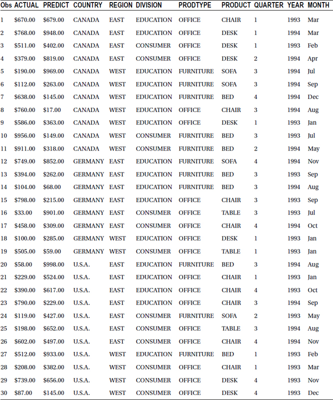
- Print the first 20 observations of Prdsale data and write your observations.
proc print data = sashelp.prdsale(obs=20);
run;
Table 5-3 lists the output of this code.
Table 5-3. Output of PROC PRINT on prdsale Dataset – 1st 20 observations

Observations from Table 5-3:
- The data set contains monthly actual and predicted sales figures along with product types and regions.
- The product type in the first 20 records is furniture, and the product is sofa.
- It looks like the data is from 1993 and onward.
- What is the size of population?
proc contents data=sashelp.prdsale varnum;
run;
The size of the population in this example is the total number of records. Proc contents show there are 1,440 records in total. Refer to Table 5-4 for the output.
Table 5-4. Results of PROC CONTENTS on predsale Dataset With varnum Option

- Filter the data and take a sample (where country=Canada).
data prod_sample;
set  sashelp.prdsale;
where country='CANADA';
run;
Here is the log file for the previous code:
NOTE: There were 480 observations read from the data set SASHELP.PRDSALE.
      WHERE country='CANADA';
NOTE: The data set WORK.PROD_SAMPLE has 480 observations and 10 variables.
NOTE: DATA statement used (Total process time):
      real time           0.67 seconds
cpu time 0.10 seconds - Take a random sample of size 30.
proc surveyselect data = sashelp.prdsale
method = SRS
rep = 1
sampsize = 30 seed = 12345 out = prod_sample_30;
id _all_;
run;
Note The method SRS represents the type of sampling. SRS stands for Simple random Sampling. Seed will make sure that we will have the same random sample drawn again. To refer to same sample, we need an index. Seed will make sure that same sample of 30 observations is drawn again.
Table 5-5 lists the output.
Table 5-5. Result of PROC SURVEYSELECT on prdsale
The SURVEYSELECT Procedure
Selection Method
Simple Random Sampling
Input Data Set
PRDSALE
Random Number Seed
12345
Sample Size
30
Selection Probability
0.020833
Sampling Weight
48
Output Data Set
PROD_SAMPLE_30
The following SAS code prints the sample prod_sample_30.
proc print data=prod_sample_30;
run;
Table 5-6 lists the output of this code.
Table 5-6. Output of PROC PRINT on prod_sample_30 Dataset
Observations:
This sample data output clearly gives a better picture of the overall population rather than printing the first few observations. We can see various product types, various countries, and so on.
- Identify the continuous, discrete, and categorical variables.
Here are the continuous variables:
- Actual (Actual Sales)
- Predicted (Predicted Sales)
These two variables are continuous as they can take any real values. For example, the sample values can be $200, $201, or $201.5.
Here are the numerical discrete variables:
- QUARTER
- YEAR
These variables can take a set of values only. Quarter can take 1 or 2; it can’t be equal to 1.5. Hence it is a discrete variable. Year is also a discrete variable.
Here are the categorical variables:
- COUNTRY
- REGION
- DIVISION
- PRODTYPE
- PRODUCT
These are not numeric type of variables.
- Which are independent variables? What are dependent variables?
- Actual and Predicted sales is the effect or the dependent variables.
- The independent variables make up the rest of the list.
- The sales here depend on country, region, product month, year, quarter, and so on. These all are independent variables.
- Calculate a parameter (mean actual sales of the population).
proc means data=sashelp.prdsale ;
var actual;
run;
Means is a SAS procedure name. In this example we have given the variable name as actual. The PROC MEANS procedure will act on this variable to find the mean.
Table 5-7 lists the output of this code.
Table 5-7. The Result of PROC MEANS on prdsale
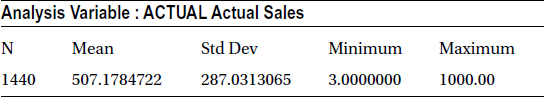
The mean sale of the population is 507.17. Details about averages will be presented later in this chapter.
- Calculate a statistic (mean actual sales of the sample).
proc means data=prod_sample_30 ;
var actual;
run;
The output of this code is listed in Table 5-8.
Table 5-8. Mean and Standard Deviation on prod_sample_30; Variable = actual

The mean sale of the sample is 451.8.
- How close is the statistic to a parameter? Is it a good estimate?
- The statistic is not very close to parameter. The sample average sale does not really represent the overall population average sales.
- There is almost an 11% difference between parameter and statistic.
- An increase in sample size might help get a good estimate. Increasing the sample size to 100 might be a better option.
- The following SAS code extracts a sample of size 100 from prdsale dataset and then calculates the mean.
/* Simple Random Sample; Size is 100 */
proc surveyselect data = sashelp.prdsale
method = SRS
rep = 1
sampsize = 100 seed = 12345 out = prod_sample_100;
id _all_;
run;

proc means data=prod_sample_100 ;
var actual;
run;
Table 5-9 lists the output of SAS code for calculating the mean and standard deviation of variable actual.
Table 5-9. Mean and Standard Deviation on prod_sample_100; Variable = actual
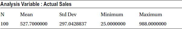
The average sales estimate (the statistic) looks closer to the overall sales of the population. The new difference is less than 5 %
There are three methods of Statistical analysis: descriptive, inferential, and predictive. In descriptive statistics methods, the data is simply summarized using statistical central tendencies and variations. In inferential statistics, a sample is drawn from the population to infer on the full set of data or population. Predictive statistics, as expected, can predict the dependent variable using methodologies such as linear and logistic regression. Some of these terms might appear strange at this point, but they will be explained in detail in the coming chapters.
Descriptive Statistics
Descriptive statistics is the right solution for presenting an overall picture about a set of data. These methodologies represent summaries, which give a fair picture about a given population. The business insights earned from the analysis of data will be in the form of tables and charts. Descriptive statistics output might help draw useful inferences, but this output in itself is not an inference.
Here is a sales example. Descriptive statistics, applied on one year’s worth of sales data, might include average sales in the last 12 months, maximum and minimum sales of the past 12 months, and so on. The business expert can infer on the performance on his or her business, based on this analysis.
The following are the important measures or outcomes of descriptive statistics:
- Measures of central tendency: Mean, median, mode, and midrange
- Measures of variation: Range, variance, standard deviation, z-scores
The next chapter will examine these terms in more detail.
You now know it is not always easy to analyze a whole population every time because of various constraints. It is therefore better to analyze a representative sample and draw inferences on the entire population. If done carefully, it can be the right decision most of the time. But since only a portion of the data is analyzed, inferences drawn on the whole data set, factors such as sample size and errors, become very important.
- Example 1: A bottling machine is supposed to fill 300 ml of soft drink in every bottle. The population size is a few thousand per day. You took a representative sample of 400 bottles and found that the sample average is 300.5 ml. Is the machine performing well?
- Example 2: Two notebook computer buyers, among a sample of 300, reported a problem with the screen. Is that a reason for concern? Based on this, can you draw the conclusion about the screen quality on a population size of about 10,000 at least?
Predictive statistics is the science of predicting future results, based on historical events. Predictive modeling or model building is like driving a car while looking into the rear-view mirror, expecting that the road ahead will be same as the road that has already been traveled on. Predictive statistics tries to predict a dependent variable or outcome by using a combination of independent variables or predictors. The historical data needs to be developed into a mathematical equation between Y (dependent variable) and Xi (independent variables).
Various techniques can be used to build the predictive model. Regression, logistic regression, and time-series analysis are good representative samples. A classic example of using predictive statistics is a bank building a credit risk model to decide whether to offer a loan to an individual.
Solving a Problem Using Statistical Analysis
This section discusses the main steps involved in statistical data analysis, also known as business analytics problem solving.
Setting Up Business Objective and Planning
Any data analysis problem begins with the business objective. Why am I doing this analysis? What is in and out of scope? Do I have enough expertise available to perform the analysis? What are the challenges? How can I implement the results? Is all relevant data available? If it is available, is it reliable? Several questions such as these abound.
The scope and analysis design or approach is the major outcome of this process.
The data that is required for analysis can be gathered after deciding the objective and scope. The data might not be perfect for analysis, whether in format, quality, or completeness. There are bound to be some missing values, outliers, and other noise factors in the data set. Starting basic data exploration, validating it for accuracy and consistency and identifying all the issues are important tasks in building a model. All the issues must be resolved before going to analysis. The following are the major steps involved:
- Collect the data.
- Explore the data.
- Validate the data.
- Clean the data.
Descriptive Analysis and Visualization
Understanding and gaining insights into the data before moving on to building a model are important tasks. Understanding each variable and their relationships is also necessary. The following are the major steps:
- Visualize the data and gain simple insights.
- Perform simple descriptive statistics.
- Perform univariate analysis for each variable.
- Create derived variables and metrics if necessary.
- Find the correlation between the variables.
This step deals with building a model to address the objective. You need to identify the most appropriate analysis technique, identify the dependent variables, and remove any redundancies. The final step is to build the best fit. Model iterations are sometimes necessary. Interpreting the model helps to know the most impacting predictor variables. The following points summarize this step:
- Identify the modeling technique.
- Build the predictive model.
- Iterate the model and find the best fit.
- Interpret the model.
The following are the questions to be answered in this step. How good is the model you have just built? Is it good only on the sample data that is used to build this model? Can you get a similar but different sample and test the accuracy of the model? How robust is my model with regard to the accuracy of prediction? Understand the following terms in connection with this step:
- In-time validation: This involves taking a sample that looks the same as the development sample from a similar time period. Sometimes, the in-time sample is 20 to 30 percent of the overall records considered for analysis; the rest is used in model building. The validation using an in-time sample is in-time validation.
- Out-of-time validation: This method takes a sample from a different time period for model validation. Sometimes, the model is perfect only on the development and in-time validation samples. Cross-validation of sample from a different time period helps test the real robustness of the model.
The model is ready when it has passed all the tests of validation. It can now be used for the business objective it was built for. The model can be implemented and applied into the production systems for trial runs in the actual business environment. Finally, it needs to be documented and handed over to the end users.
Figure 5-1 shows all the steps used in the model building. This book will touch upon most of them.
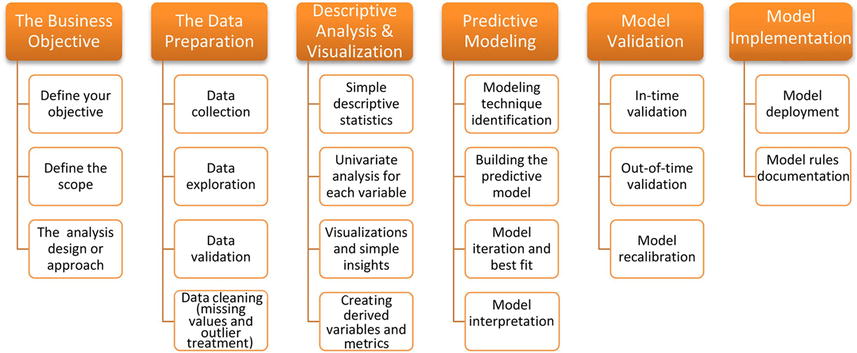
Figure 5-1. Steps Used in Model Building
An Example from the Real World: Credit Risk Life Cycle
Consider an example of credit risk model building. Every bank wants to analyze how risky it is to offer a loan or approve a credit card to an applicant. The approval or rejection is normally based on a predictive model, which may contain 15 to 20 variables that are filtered from 400 independent variables. The following are the basic steps in building a credit risk model.
Business Objective and Planning
The objective is to predict the risk factor on every potential applicant. Determining the portfolio size, creating growth plans, and simulating the competitive and business environment can be other objectives. Detailed project management plans can also be made at this stage.
Data Preparation
The required data is collected from customer historical records with the bank, in-house applications, and customer facing retail applications or any other federated data marts. Data from these multiple sources is likely to have heterogeneous data formats. Hence data cleansing and transformation is a must. Correction for outliers, missing value treatment, and other data cleansing steps are done at this stage. Creating dummy or derived variables is also done if required.
Descriptive Analysis and Visualization
The performance window is decided, which tells us how much historical data should be considered for analysis. The usual performance window for this kind of analysis is 12 months. Defining the good and bad accounts that will be used in model building later is done at this stage. Analysts must decide whether the population needs to be divided into various segments. If yes, then the segmentation variables are also identified.
This step identifies the most important factors that will have the most significant effect on the probability of default. For example, with the number of current loans versus age, consider which one of these two will be the most important factor in determining the credit risk.
Predictive Modeling
The predictive modeling step involves building a logistic regression model, which will give the probability of default using the finalized list of dependent variables. Building this model will be discussed in detail in later chapters. Typically three to four different models are built at this stage. The best one that gives the least error is selected.
How good is the model performing on the data other than the sample that was used for its construction? Statistics like Chi square, KS and rank ordering are used to validate the model performance. KS tells how good the model is in separating the good from the bad, while the PSI value gives you an idea of the similarity of the current population (the real production data) versus that of the development sample.
- KS test: KS stats for Kolmogorov-Smirnov. This is used to find whether the model is efficiently separating good from bad. The higher the KS, the better the model
- PSI: PSI stands for Population Stability Index. Banks have to make sure the current population on which the credit scoring model will be used is same as the development time population. If there is a drastic shift in the population, then the scorecard (model) might not be valid anymore.
Model Implementation
The final step is to start using the credit risk model, which will convert the risk into a score. The model, at this stage, is given to the IT developers for implementation. Whenever there is a new credit card application, the system, equipped with this model, will automatically calculate the credit score. Using this credit score the bank’s front end staff will approve or decline the application
Conclusion
This chapter defined some basic statistical terms. They will be useful in all the chapters that follow. It also covered the basic steps that are followed in solving business analytics problems. This was done with the help of a real-life bank scenario. The next few chapters will discuss descriptive statistics, followed by data preparation and predictive modeling. All the steps mentioned in Figure 5-1 will be discussed along with its terminology, which at this stage might look somewhat alien.