2	Matrix Models and Structured Population Dynamics

If a population or species is in decline and at risk of extinction, it is clear what we need to do: increase the birth rate, decrease the death rate, or both. But exactly whose birth or death rate are we talking about? For example, given limited human and financial resources, would it be more effective to create additional good nesting sites so more adult birds can breed each year, to shield eggs from predators so that each nest produces more offspring, or to augment food supply so that juveniles have a better shot at surviving to breeding age?

Trying to answer these questions in advance, rather than by trial and error, is an increasing part of the conservation biologist’s job. This chapter focuses on a type of model that is widely used for this task (Morris and Doak 2002): matrix models for the dynamics of structured populations. “Structured” means that the model incorporates differences among individuals. Models based on differences in age were developed centuries ago for the study of human populations—one basic result is credited to Euler (1707–1783)—and we will start by considering that case. To understand structured population models we need some aspects of matrix theory. We review this from the ground up, beginning by defining matrices and reviewing basic matrix algebra. We then consider some applications, including conservation planning, and finally some generalizations of the model.

This chapter and the next introduce our modus operandi of using a small number of in-depth case studies as the vehicle for presenting different types of models and for motivating the study of their properties. To indicate the range of applicability for matrix models, we will not give you a quick survey of examples from other areas of biology, or even a list of books and articles with other applications. Instead, we follow this chapter with one where matrix models (and other kinds of model) are applied in a totally different biological context. Within our own field of biology we feel confident about choosing good “role models” for you to study. For the rest, you’ll have to explore the literature and decide for yourself.

2.1 The Population Balance Law

The starting point for population modeling is the fundamental balance law

where N(t) is the number of individuals in the population or the population density (number per unit area) at time t. The balance law becomes a complete model when we specify formulas for the quantities on the right-hand side. The simplest model is to assume a closed population without immigration or emigration, and that the per capita (i.e., per individual) birth and death rates are constant:

Births = b × N(t), Deaths = d × N(t).

The balance law then becomes

where λ = 1 + b – d. This model is simple enough that we can solve it. Starting from any initial population size N(0) we get

N(1) = λN(0)

N(2) = λN(1) = λ(λN(0)) = λ²N(0)

N(3) = λN(2) = λ(λ²N(0)) = λ³N(0),

and so on, leading to the general solution

This is exponential population growth: defining r = log λ, we then have λ^t = (e^r)^t = e^rt and so

N(t) = e^rt N(0).

(Note that “log” means the natural (base-e) logarithm; we will use log₁₀ to indicate base-10 logarithms.)

Growth cannot go on forever, so [2.3] cannot be valid forever if λ > 1. This kind of limitation bothers biologists much more than it bothers physical scientists, who are used to the idea that different models for a given system may be valid in different circumstances. Anderson and May (1992, p. 9) compare simple biological models to Newton’s first law of motion:

A body remains in its state of rest or uniform motion in a straight line, unless acted on by external forces.

Exponential population growth has the same character—it tells us what happens if current conditions persist without change:

A closed population of self-reproducing entities—such as viruses, cells, animals, or plants—will grow or decay exponentially at a constant rate, unless a change in conditions alters the per entity birth or death rate.

Therefore, more general models are derived by considering the factors that can alter the average per entity birth and death rates.

2.2 Age-Structured Models

The biological theme of this chapter is that per entity birth and death rates are affected systematically by differences among individuals, such as their age. To take effects of age into account we need to describe the population by a state vector listing the numbers of individuals of each age. It is natural (but not necessary) to use years as the time unit; the state variables are then n_a(t), the number of a-year-old individuals in year t, with a running from 0 to the maximum possible age A.

For now we continue to assume a closed population without immigration or emigration. The model’s dynamic equations are bookkeeping expressed in mathematical symbols, as in the salmon model in Chapter 1. Consider one of the authors: 50 years old in January 2004. In order to reach that state, he must have been 49 years old in January 2003 and survived the next year. Consequently

where p₄₉ is the probability that a 49-year-old survives to age 50. In general, this line of reasoning tells us that

where p_x is the probability that an x-year-old individual survives to be age x + 1.

To complete the model we need to specify the number of births each year. If we assume that per individual birth rates are only a function of age, we can define f_a to be the average number of newborns next year, per age-a female this year. Then we have

Two conventions can be used: count everybody, or only count females—in which case f_a only includes female offspring. The females-only convention is by far the more common, and we will always use it here.

Exercise 2.1. Find at least two important assumptions that are necessary for [2.5] to be true.

Exercise 2.2. Define l₀ = 1, l_a = p₀p₁p₂· · · p_a−1, the probability of an individual surviving from birth to age a. Explain in words why

Exercise 2.3. The general theory developed later in this chapter tells us that in the long run a population governed by the age-structured model typically grows exponentially, as in [2.3]. In particular, n₀(t) = cλ^t will hold (with greater and greater accuracy as time goes on), for some λ and c. By substituting this approximation for n₀(t) into [2.7], show that the long-term population growth rate λ satisfies the equation

This is called the Euler, Lotka, or Euler-Lotka equation.

Exercise 2.4. (a) Show that the left-hand side of [2.8] is a decreasing function of λ by computing its derivative with respect to λ. (b) Compute the values of the left-hand side in the limits λ → 0 and λ → ∞. (c) Explain why (a) and (b) imply that [2.8] has one and only one positive real solution.

2.2.1 The Leslie Matrix

It is convenient and informative to express the age-structured model in matrix notation. In this form it is called the Leslie matrix model, after British ecologist P. H. Leslie who popularized age-structured models for animal populations in the mid-twentieth century.

First we need to review a bit about matrices. A matrix is a rectangular array of numbers. A matrix A with entries a_ij is said to have size m × n if it has m (horizontal) rows and n (vertical) columns. Thus the row index i takes the values 1, 2, . . . , m (1 indicating the top row) and the column index j takes the values 1, 2, . . . , n (1 indicating the leftmost column). A matrix with one column is called a column vector, and a matrix with a single row is called a row vector.

Matrix algebra was invented for studying systems of linear equations in several unknowns, such as

Solving one such equation in one unknown is a snap:

Matrix algebra lets us make [2.9] look like [2.10], so that we can solve it in the same way. We put the coefficients in [2.9] into a matrix

and put the variables and right-hand side into vectors Matrix-vector multiplication is then defined so that [2.9] is equivalent to the single matrix equation:

The definition that makes [2.9] and [2.12] mean the same thing is the following: if x = (x₁, x₂, . . . , x_n) is a column vector and A is a matrix with n columns, then Ax is the column vector

Algebraically, that works out to the following formula: for a matrix A with n columns and a column vector x of length n, Ax is the vector whose ith element is

where A_ij is the number in the ith row and jth column of the matrix A. Equation [2.14] says that the ith element of Ax is the inner product of the ith row of A with x, where the inner product of two vectors v and x of length n is defined as

This expression is sometimes called the dot product, and the alternate notations or (v, x) are also used.

The inner-product interpretation of [2.14] is how people are usually taught to do matrix-vector multiplication by hand. For example (and make sure that you understand this example!),

However, the conceptual definition [2.13] is essential for understanding the biological meaning of matrix models.

So what good does this do us? Suppose that we could find a multiplicative inverse to A—a matrix A⁻¹ such that A⁻¹(Ax) = x for any vector x. Then we could solve [2.12] the same way we solved [2.10]: just multiply both sides of equation [2.12] by the inverse of A to get the solution x = A⁻¹b. Figuring out when such inverses exist and how to compute them was one of the major accomplishments of nineteenth-century mathematics.

As is often the case in mathematics, a tool invented for one purpose turns out to be useful for many others. Notice that the equation [2.6] for births in the age-structured model has the same form as [2.14]. The survival equation [2.5] is also a sum, with only one term. So we can express these in matrix notation by putting the survival and birth rates in the right places:

or simply

where L is the matrix in [2.17], and n(t) is the population vector (n₀(t), n₁(t), . . . , n_A(t)). The top row of the matrix contains the births, and the other nonzero entries are survival.

For example, consider a plant with a maximum age of 2—this might be a plant that flowers once, at either age 1 or age 2, and then dies. Suppose that newborn offspring (age 0) have a 50% chance of surviving to age 1; age-1 plants produce f₁ offspring each on average, and have a 25% chance of surviving to age 2, and age-2 individuals have f₂ offspring each on average. The Leslie matrix is then

Definition [2.13] tells us how to “read” a matrix like [2.19]. Since n_i(t) multiplies the ith column of the Leslie matrix, the ith column of L gives the individuals of each age “next year” resulting from a single age-i individual “this year,” as a consequence of their survival and fecundity. So the first column says that for each age-0 individual this year, there will be (on average) half a 1 year old next year—the ones that survive. The second says that for each age-1 individual this year, the population next year will have f₁ age-0 individuals (the offspring of age-1 individuals) and 0.25 age-2 individuals (the age-1 individuals who survive to next year). Age-2 individuals all die, so their only contribution to next year’s population is their offspring (f₂ per 2 year old). In the same way, the jth column of the general Leslie matrix [2.17] says that for each j year old “this year,” next year’s population will have f_j offspring (age 0) and p_j survivors (age j + 1).

Note that it does not matter how survivorship and breeding at a given age are related to each other. For example, it could be the case in [2.19] that half the age-1 individuals reproduce and then die (having 2f₁ offspring each, on average) while those that do not reproduce have a 50% chance of surviving to age 2. Or it could be the case that all age-1 individuals reproduce, and all have a 25% chance of surviving to age 2. Either way the matrix is the same.

Exercise 2.5. Verify that the following are correct in three different ways: using [2.13], using the inner-product method illustrated in Equation [2.16], and by writing a script to do the calculations on the computer.

Exercise 2.6. Write a script file to run simulations of the biennial plant model [2.19] with f₁ = 1, f₂ = 5, starting from a single age-1 individual at time 0. Have the script plot as functions of time (1) the log of the total population size N(t) = n₀(t) + n₁(t) + n₂(t), and (2) the fraction of individuals of each age, w_i(t) = n_i(t)/N(t), i = 1, 2, 3, for t = 1 to 50. What long-term properties of the population do you see in your simulation results?

Exercise 2.7. Write down the Euler-Lotka equation [2.8] for the biennial plant model [2.19] with f₁ = 1, f₂ = 5, and numerically solve it for the value of λ. How does this compare to the rate of population growth that you saw in your simulations? [You can find λ approximately by having your script compute the left-hand side of [2.8] at a finely spaced set of λ values, and finding one at which the sum is closest to 1. Or if you’re adventurous, find a function in your scripting language that finds the roots of univariate functions, e.g., uniroot in R or fzero in MATLAB.]

2.2.2 Warning: Prebreeding versus Postbreeding Models

The interpretation of the f’s depends on when births occur relative to the annual census time. Suppose we census the population on January 1 each year. In humans, births occur year round, so f_a should be the average number of births over the coming calendar year, to an individual whose age was between a and a + 1 on January 1, but only counting offspring that survive until January 1 of next year. So f_a is the sum over all such individuals of

and so on.

In other cases it is more accurate to assume a once-per-year seasonal “pulse” of births, as if all offspring for the year were born at once. Let m_a be the number of offspring that an a year old has in the current birth pulse. If we census the population immediately after the pulse (postbreeding census) then

f_a = p_a [survival to next year]

×m_a+1 [# offspring in next year’s birth pulse].

But if we census just before the pulse (prebreeding census), then

f_a = m_a [# offspring now—but not counted until next year]

×p₀ [fraction of offspring who survive to be counted].

Both of these are valid under their assumptions about census timing, and both are used. As a result, formulas for things like life expectancy, population growth rate, and so on, exist in two different versions for prebreeding and postbreeding models. An additional complication is that some authors (e.g., Caswell 2001) number age-classes starting at 1 rather than 0, so that their n₁(t) is equivalent to our n₀(t). Even experts get confused by all these options, and many books and papers include a mix of formulas based on incompatible assumptions. So when you see f₄ in a book or paper, it’s important to check what the author intends it to mean.

2.3 Matrix Models Based on Stage Classes

In most applications to nonhuman organisms, the oldest age A really consists of individuals aged A or older, due to lack of data. The meaning of “extreme old age” is that most individuals die before they get there, so there always are relatively few observations of what happens to extremely old individuals. For example, suppose during your study of a lizard population, there is one hardy 4 year old who lives to be 5, then lives to be 6, and then dies, while all other individuals die before they reach the age of 4. So would you then take p₄ = 1, p₅ = 1, p₆ = 0? A better option is to assume that all individuals above some age are identical, so that you can get a reasonable estimate of their average survival probability.

Collapsing all ages above some cutoff into one “age-class” is our first example of the tradeoff between model error and parameter error. Model error means errors due to incorrect assumptions, where the model simplifies or omits known aspects of reality. Combining all individuals of age 3 or above is likely to create model error, because we have no grounds for believing that there really are no systematic differences between a 3 year old and a 5 year old. Parameter error means errors due to parameters being estimated inexactly from a limited set of data. By combining all 3+ year olds, we avoid the parameter errors that would result from estimating p₄, p₅, and p₆ from a sample of size 1. The resulting model has a category of individuals who are likely to be fairly similar, with parameters for the category being “average” or “typical” values for members of the category. It is always possible to reduce model error by making a model more complex, but parameter error usually goes up because you have to somehow estimate more parameters from the same amount of data. We discuss this tradeoff more fully in Chapter 9.

More generally, individuals can be classified by their stage in the life cycle. Sometimes there really are discrete life stages, such as caterpillar-cocoon-butterfly (or more generally larva-pupa-adult in insects). But sometimes it is just a group of individuals defined by some measurable feature, such as length or weight, that is the best available attribute for predicting their fate over the next period of time.

The most common attributes for defining categories are measures of individual size. These have long been popular in the forestry literature, because size is generally much better than age for predicting tree growth and mortality. Now size is used also for animal populations, with recent examples including sea turtles, desert tortoise, geese, corals, copepods, and fish (Caswell 2001). Size categories are usually defined so that between one census and the next individuals can grow or shrink by at most one category, and all newborns are in the smallest category, but this is not always the case. For example, Valverde and Silvertown (1998) used size-classified matrix models for the woodland herbaceous plant Primula vulgaris in which individuals could grow by two categories, in order to study how Primula population growth was affected by the degree of forest canopy closure. For one of their study sites (Woburn Wood), the projection matrix for 1993 to 1994 was with the categories being defined by plant area (see the right-hand side of Table 2.1). As with our hypothetical model [2.19] we “read” this matrix by recognizing that each column specifies the contribution of one category to next year’s population.

A useful way to graphically represent a stage-classified matrix model is the life cycle graph in which each “node” represents a stage, and arrows show possible changes in stage for individuals between one time interval and the next. Figures 2.1 and 2.2 show two examples. By convention, staying put in a stage is drawn as an arrow, but deaths are omitted on the assumption that no life stage is invulnerable. Also note that there is no distinction in the diagram between survival and fecundity. Since a basic premise of the model is that an individual’s stage classification provides complete information about its future prospects, it does not matter (in the model) if a small individual is a newborn or an older individual who shrank back down to newborn size. The life cycle diagram represents your idea of a good way of classifying individuals. If there are discrete stages, it is probably a good idea to use those in the model. Otherwise, experience suggests that the most important issue is selecting which trait to use as the basis for classifying individuals (e.g., age versus size). The trait used for classifying individuals is sometimes called the individual state variable or the i-state variable.

Table 2.1 Two examples of stage classifications based in part on individual size. Asterisks indicate reproductive categories. The two left columns give the categories used by Doak et al. (1994) for desert tortoise in the western Mojave desert, which were the same as those used by the Bureau of Land Management in the population monitoring program that provided the data for the model. The two right columns give the categories defined by Valverde and Silvertown for the forest herb Primula vulgaris.

Figure 2.1 The standard size-class model. Size categories are broad enough that individuals can’t change by more than one category between population censuses, and all newborn individuals are in the smallest size class. These all look the same apart from the number of “stages”.

Figure 2.2 Stage-structured model for killer whales (from Brault and Caswell 1993). The stages recognized were 1 = yearling, 2 = juvenile, 3 = mature female, and 4 = postreproductive female.

Given the right data, alternative choices of i-state variable can be compared objectively. For example, if you know an individual’s size, can you predict her fecundity more accurately if you also know her age? Caswell (2001, section 3.3) presents several examples of this kind of comparison. However, the classification is often dictated by circumstances. For example, Doak et al. (1994) based their model on data that had already been collected by the Bureau of Land Management. They had no choice but to use size as their i-state variable, with the categories used in the BLM surveys (Table 2.1). Valverde and Silvertown (1998) based their classification on knowledge of the species’ natural history, with class boundaries chosen so that each category had sufficient sample size for estimating matrix entries.

Having chosen a stage classification, the model is completed by specifying the projection matrix entries a_ij,

a_ij = number of type-i individuals at time t + 1, per type-j individual at time t.

Contributions from j to i may be survival, fecundity, or a combination of these. As in the age-structured model, we assume (for now) that the a_ij are constant. The fundamental balance law is then

The projection matrix A is defined to be the n × n matrix with entries a_ij, and the model then becomes

Estimating the value of matrix entries is a subject in itself. Entire careers (and entire books, e.g., Williams et al. 2002) are devoted to methods for analyzing census data on populations in order to estimate demographic rates. Morris and Doak (2002, Chapter 6) give some guidelines on how to conduct field studies to estimate demographic rates. The ideal situation is if individuals can be given a unique tag or mark (or come with unique markings), and you can come back later to see what happened to them. Plants sit still and wait to be counted, but with animals it is often hard to distinguish between death and emigration out of the study area.

Similarly for fecundities, the best situation is if you can identify and count the offspring of each parent. This is often possible with large animals or animals that live in family groups. For plants, a common approach is to count seeds while they are still on the parent plant. Then, assuming that (once released) a seed is a seed is a seed, you can estimate

F_i = (average number of seeds produced by a class-i plant)

× (fraction of all seeds that survive to be seedlings at the next census).

The same idea has also been used for estimating fecundity in birds: do a census of offspring in their natal nest, and decrement those counts by the overall fraction of nestlings that survive to the next census.

There are also ways to indirectly estimate parameters from population count data. Indirect methods begin by assuming that the model is valid, and then asking: What must the survival (or growth or fecundity) parameters be, in order to generate the population that I observed? This is more difficult than direct estimates and less secure, because of the a priori assumption that the model is valid. Indirect methods for structured population models are reviewed by Wood (1997) and Caswell (2001, section 6.2).

Exercise 2.8. State in words the meaning of the second and fourth columns of the projection matrix given above for Primula vulgaris in Woburn Wood.

Exercise 2.9. Draw the life cycle graph for Primula vulgaris in Woburn Wood.

2.4 Matrices and Matrix Operations

Our goal now is to derive general properties of matrix models that allow us to make connections between the matrix entries and the long-term fate of a population governed by [2.21]. For example, in conservation planning it is important to know which matrix entries have the greatest impact on whether the population is growing or shrinking, so that those can be targets for remediation efforts (e.g., striving to increase the survival during particularly important stages of the life cycle).

Rewriting the balance equations [2.20] in matrix form [2.21] is more than a convenience, because the algebra of matrices (called linear algebra) has a lot to tell us about the equations. This section reviews some concepts and results from linear algebra that will give us much insight into the balance equations for populations. Moreover, these results will be employed in Chapter 3 in an entirely different setting, to model the gating of membrane channels in neurons.

2.4.1 Review of Matrix Operations

Addition and subtraction of matrices are done element by element, and are therefore only defined for matrices of the same size:

Multiplication of a matrix by a scalar (real number) is also element by element:

Examples are

Matrix multiplication is more complicated. The product C = AB is defined if the number of columns of A is equal to the number of rows of B. If A = (a_ij) has size m × n and B = (b_ij) has size n × r, then C = A · B has size m × r and

Note that if B has only one column, this reduces to the definition of matrix-vector multiplication [2.14]. Thus, another definition of matrix multiplication is the following:

Our attitude is that matrix multiplication is usually best done on the computer. It is important to understand the conceptual definition [2.26] and the algebraic formula [2.25], but when working with actual numbers, it is easier and less error-prone to use a computer language that includes matrices and matrix multiplication.

Matrix operations share many properties with the familiar arithmetic of real numbers. For example,

• Matrix addition is associative [A + (B + C) = (A + B) + C] and commutative [A + B = B + A].

• Matrix multiplication is associative [A(BC) = (AB)C] and distributive over addition [A(B + C) = AB + AC, (A + B)C = AC + BC].

However, matrix multiplication is not commutative—typically AB ≠ BA. Indeed, unless A and B are square matrices of the same size, either one of the produ AB and BA will be undefined, or the two products will be matrices of different sizes. But even in the case of square matrices commutativity typically does not hold. Here is a simple example:

but

However, scalar multiplication is commutative in the sense that A(cB) = c(AB).

2.4.2 Solution of the Matrix Model

Having defined matrix multiplication, we can now easily write down the solution to the matrix model [2.21], in the same way that we solved the unstructured model [2.2]. Starting from some initial population vector n(0) we get

leading to the general solution

where A^t denotes the product of A with itself t times. We can form these products because A is a square matrix, and the order of operations in computing the products does not matter because matrix multiplication is associative.

2.5 Eigenvalues and a Second Solution of the Model

The most basic question we can ask about a population is whether it will grow or become extinct in the long run. The solution of the matrix model shows that the answer depends on the behavior of A^t, the powers of the projection matrix as t increases. We can determine the properties of A^t through the eigenvalues and eigenvectors of the matrix A.

A number (possibly complex) λ is an eigenvalue of A if there is a nonzero vector w such that Aw = λw, and w is called the corresponding eigenvector. Eigenvectors are defined only up to scaling factors: if w is an eigenvector for λ then so is cw for any number c ≠ 0. An n × n matrix A must have at least one eigenvalue-eigenvector pair, and it can have up to n (see this chapter’s Appendix for an explanation of why this is true). The typical situation is to have n distinct eigenvalues each with a corresponding eigenvector—this is typical in the sense that if matrix entries are chosen at random according to some smooth probability distribution, the probability of the resulting matrix having n distinct eigenvalues is 1.

There is a useful formula for the eigenvalues of a 2 × 2 matrix A. If T = a₁₁ + a₂₂ is the trace (sum of diagonal elements) and Δ = a₁₁ a₂₂ − a₁₂a₂₁ is the determinant then the eigenvalues are

Back to equation [2.21]. Assuming there are n distinct eigenvalues, the corresponding eigenvectors w_i are linearly independent, which means that for any n(0) it is possible to find constants c_i such that

Then

Comparing [2.30] with [2.31] we see that going forward one step in time corresponds to multiplying all the coefficients c_i by the corresponding eigenvalue λ_i. We can go from t = 1 to t = 2 in the same way, getting

and so forth. Thus the solution of the matrix model is

An eigenvalue λ₁ is called dominant if |λ_i| < |λ₁| for all other eigenvalues of A. If so, it follows from [2.33] that the long-run behavior of the population is determined by the dominant eigenvalue and its eigenvector:

The meaning of ~ in equation [2.34] is that as t → ∞ the relative error goes to zero.

Equation [2.34] tells us two things about the population. First, in the long run the total population size grows exponentially at rate λ₁, just as in the unstructured model [2.2]. Second, the population vector becomes becomes proportional to w₁; in particular, the relative numbers in each stage become constant. For that reason, w₁ is called the stable stage distribution.

The Perron-Frobenius theorem from linear algebra provides an easy-to-check condition which guarantees existence of a dominant eigenvalue. A matrix A is called power-positive if there is an integer m > 0 such that all entries of the matrix A^m are strictly positive. The most important result is the following:

If a non-negative, square matrix A is power-positive, then A has a unique dominant eigenvalue λ which is real and positive, and the eigenvector w corresponding to λ has all positive entries.

This criterion for existence of a dominant eigenvalue is especially useful because power-positivity depends only on which elements in the matrix are positive, not on their numerical values. It is also useful that there is a simple test to determine if a non-negative matrix is power-positive (Horn and Johnson 1985, p. 520), which is easy to implement on the computer:

If A is a non-negative square matrix with n rows and columns, then A is power-positive if and only if all entries of A^n2−2n+2 are positive.

Because eigenvectors are defined only up to multiplication by a constant, the statement that the dominant eigenvector has all positive entries really means that all entries in any dominant eigenvector have the same sign. A software package may give you an eigenvector (call it w*) with all negative entries, in which case w = − w* is the strictly positive eigenvector guaranteed by Perron-Frobenius¹.

Exercise 2.10. Write a script to verify that the following projection matrix is power-positive:

Exercise 2.11. Find a 4 × 4 Leslie matrix L₁ that is power-positive, and a second Leslie matrix L₂ that is not power-positive. In the latter case, verify your conclusion by writing a script that computes and prints the smallest value in the matrix for each j = 1, 2, . . . , n² – 2n + 2. What happens to the age structure, starting from a single newborn, in your non-power-positive example? [Note: a Leslie matrix is a matrix of the form [2.17], in which all of the p’s are positive, and at least one of the f’s must be positive.]

Exercise 2.12. According to Lande (1988) females of the Northern Spotted Owl begin breeding at age a = 3, and are estimated to have an average of 0.24 female offspring per year until they die (f_a = 0.24 for a ≥ 3). The survival probability from birth to age 3 is estimated to be 0.0722, and the annual survival probability of adults (age 3 or older) is 0.942 (these values refer to the notational conventions that we used in the age-structured model, so that a newborn individual is 0). This owl has been controversial, because of the conflict between the need to preserve old-growth forests as habitat for spotted owl, and the interest of logging companies in harvesting those forests.

(a) We told you that l₃ = p₀p₁p₂ = 0.0722 but not the values of the individual p’s. That is because any choice of p’s with this product will result in the same population growth rate. Why is that true? (Note: the answer to this question should be verbal; no formulas are needed).

(b) Construct a projection matrix for the population based on the estimates above.

(c) Compute the owl’s long-term growth rate λ from the projection matrix. Does it appear that the population is safe, or in danger of extinction?

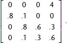
Exercise 2.13. Killer whales (Orcinus orca) are long-lived marine mammals that live in stable social groups called “pods.” Their stable social structure and the fact that individual whales can be photo-identified makes them especially well suited to scientific study. Demographic data on killer whale populations in the coastal waters of British Columbia and Washington state have been collected since 1973. Brault and Caswell (1993) used the 1973–1987 data and a stage-structured matrix model to investigate several demographic questions concerning the whales. They model the females with a mixed age-stage classification: yearlings, juveniles (past the first year, but not mature), mature, and postreproductive. The life cycle graph is shown in Figure 2.2 and the projection matrix A is given below:

Write a script file that

(a) computes the dominant eigenvalue λ and stable stage distribution w for the whale population;

(b) projects the population dynamics for the next 50 years assuming that the current population vector is x₀ = (10, 60, 110, 70);

(c) plots on three separate graphs the projected changes over time in

• N(t) = total population size in year t,

• the annual population growth rate λ(t) = N(t + 1)/N(t),

• the proportion of individuals in each stage.

Does the population structure become stable? How does it change over time? How quickly does the annual growth rate λ(t) converge to the dominant eigenvalue λ?

Exercise 2.14. Rerun your script for killer whale population dynamics with the following initial population vectors:x₀ = (250, 0, 0, 0), (0, 250, 0, 0), (0, 0, 250, 0), and (0, 0, 0, 250). Compare and contrast the four population projections—for example, (a) consider the stage distribution and its stability; (b) which stage seems to be the most important in terms of the future growth of the population?

Exercise 2.15. Consider a possible harvest from the killer whale population, consisting of individuals from a single stage, for example, all juveniles or all reproductive adults. Suppose that the initial population structure is the stable distribution w with a total of 250 individuals. What is the maximum number of juveniles that can be taken each year such that the population is not driven to extinction? What is the maximum number of reproductive adults? Note: Assume that harvest will take place after the breeding season, so that the model becomes x(t + 1) = Ax(t) − h where h = (h₁; h₂; h₃; h₄) is a vector of the number of individuals harvested from each stage each year, h_i. Assume that h is constant: same harvest each year.

2.5.1 Left Eigenvectors

There is a definition of left eigenvalues and eigenvectors analogous to that for right eigenvalues and eigenvectors: if vA = λv (where v is a nonzero row vector of length n) then v is a left eigenvector and λ is the corresponding eigenvalues. There are three key properties:

• The left eigenvalues of a matrix A are the same as the right eigenvalues.

• The left eigenvectors of A are the right eigenvectors of its transpose A^T. A^T is the matrix whose (i, j)th element is a_ji. That is, the rows of A become the columns of A^T, for example,

• If A is power-positive so is A^T, and hence the dominant left eigenvalue has all positive entries.

Left eigenvectors are important for the long-term dynamics of matrix models. First, they determine eigenvalue sensitivity: the extent to which each matrix entry affects the dominant eigenvalue. Let v and w be the left and right eigenvectors corresponding to the dominant eigenvalue λ of a power-positive projection matrix A. Then

where v · w is the dot product defined above [equation (2.15)].

Second, the dominant left eigenvector (when it exists) has a biological interpretation as the “reproductive value” of different stages, a concept due to R. A. Fisher. Think of different stages as alternate “investments” in long-term population growth. If you could put one dollar into any one of these investments (~ one individual in any of the stages) what is their relative payoff in the long run (relative size of the resulting population in the distant future)? The answer is that the “payoff” from a stage-j individual is proportional to v_j (see the Appendix of this chapter). In age-structured models it is conventional to scale v so that v₀ = 1, that is, so that its entries are reproductive values relative to that of a newborn.

Exercise 2.16. Compute the reproductive value vector v for the killer whale model [2.35], scaled so that v₁ = 1. How does this relate to your conclusions from simulating the population starting from different initial populations?

Exercise 2.17. Construct the projection matrix A, and then find λ, v, and w for an age-structured model with the following survival and fecundity parameters. Age-classes 0–5 are genuine age classes with survival probabilities [p₀, p₁, . . . , p₅] = [0.3, 0.4, 0.5, 0.6, 0.6, 0.7]. Note that p_j = a_{j + 1,j}, the chance of surviving from age j to age j + 1, for these ages. Age-class 6 are adults (age 6 or older), with survival 0.9 and fecundity 12.

2.6 Some Applications of Matrix Models

Table 2.2 summarizes the main theoretical results for the case of a power-positive projection matrix A. From here on λ, v, w without subscripts will refer to the dominant eigenvalue (formerly λ₁) and corresponding left and right eigenvectors, whose existence is guaranteed by the Perron-Frobenius theorem. We now present two applications of these results to biological questions that have been addressed using matrix population models.

2.6.1 Why Do We Age?

Evolutionary biologists distinguish between proximate and ultimate explanations for phenomena. A proximate explanation tells us how the phenomenon occurs—for example, the physical and biochemical processes involved in meiotic cell division as part of sexual reproduction. An ultimate explanation attempts to say why the phenomenon occurs—for example, why some species have evolved to have sexual reproduction while others have not.

Model	n(t + 1) = An(t), n(0) = n0
Solution
Eigenmode expansion
Long-term exponential growth
Stable stage distribution
Stage-specific reproductive value	Proportional to v
Eigenvalue sensitivity formula

Table 2.2 Main properties of a matrix model with power-positive projection matrix A

Models are important for developing ultimate explanations, because they let us consider the consequences of the alternatives that are not seen in nature. As R. A. Fisher observed, if we want to understand why humans have two sexes rather than three or more, we must “work out the detailed consequences experienced by organisms having three or more sexes” (Fisher 1930). To understand the “why” of traits molded by evolution, we first need to compare things as they are with the other ways things might have been. Only then can we start to hypothesize why evolution produced one outcome rather than the other.

For modeling evolution of the life cycle, the growth rate λ can be identified with Darwinian fitness: the contribution of offspring to future generations. On the reasonable assumption that matrix entries are determined by the organism’s genotype, and if multiple genotypes are present within a population, then population genetic models predict (with some caveats) that the genotype with the largest λ for its matrix becomes fixed in the population (Charlesworth 1994). The main caveat is a standard one in population genetics theory: if the most fit genotype is a heterozygote, then a stable polymorphism is maintained.

An ultimate explanation for sexual reproduction still eludes us: theories abound, and new ones are proposed as quickly as old ones are rejected. But for aging (technically called senescence), there is a widely accepted theory based on the eigenvalue sensitivity [equation [2.36]]. This explanation is derived by modeling a life cycle without aging—the alternative that is not seen in nature—and then asking whether a little bit of aging would lead to increased Darwinian fitness.

Life without aging means that females start reproducing at some age m (for “maturity”), and thereafter have constant fecundity f_j = f and survival p_j = p < 1 for all ages j ≥ m. We have assumed that p < 1 to represent an age-independent rate of deaths unrelated to aging.

The eigenvalue sensitivity formula lets us compute the relative eigenvalue sensitivities at different ages for this life cycle without any hard calculations, so long as λ = 1. Populations cannot grow or decline without limit, so λ must be near 1. The reproductive value of adults (v_i, i ≥ m) is independent of age because all adults have exactly the same future prospects and therefore make the same long-term contribution to future generations. On the other hand, the stable age distribution w_j goes down with age. With λ = 1 the number of m year olds is constant, so we can compute n_m+k(t) = n_m(t − k)p^k = n_m(t)p^k. That is, in order to be age (m + k) now, you must have been m years old k years ago, and you must have survived for the k years between then and now. Therefore

Consequently, the relative sensitivity of λ to changes in either the fecundity a_1,j or survival a_j+1,j of age-j females, is proportional to p^j−m. In both cases, as j changes the relevant w_j is proportional to p^j−m while the reproductive value v_j stays the same. This has two consequences:

1. The strength of selection against deleterious mutations acting late in life is weaker than selection against deleterious mutations acting early in life.

2. Mutations that increase survival or fecundity early in life, at the expense of an equal decrease later in life, will be favored by natural selection.

These are known, respectively, as the mutation accumulation and antagonistic pleiotropy theories of aging. In addition there is a particular form of antagonistic pleiotropy, the disposable soma hypothesis, which posits that the connection between early and late vigor is mediated by investment in maintenance and repair mechanisms at the cellular and molecular levels, such as DNA repair and antioxidant systems.

Distinguishing between these theories is difficult because they agree on the fundamental prediction: If the level of unavoidable extrinsic mortality is high then the organism is predicted to be short lived even in a protected environment, while low levels of unavoidable extrinsic mortality should lead to potentially long-lived organisms. Experiments—mainly on Drosophila—have uniformly supported this prediction (Kirkwood and Austad 2000). In addition, there is some direct support for each mechanism.

Antagonistic pleiotropy.

There is abundant evidence for antagonistic tradeoffs (e.g., Roff 2001, Chapter 3). The ideal organism would mature instantly, live forever, breed often, and have many offspring each time. In reality we never see this because improvements on one front are paid for on another. For example, early maturation typically entails smaller adult body size and hence lower fecundity. Conversely, experimental selection against early fecundity in Drosophila led to increased fecundity later in life. Similar results have been obtained on other insects, birds, and mice (Roff 2001).

Disposable soma.

A unique prediction of this theory, also supported by numerous studies, is that intrinsically long-lived organisms should have higher levels of cellular-level maintenance and repair processes. For example, DNA repair capacity correlates with lifespan in mammals, as does the level of poly(ADP-ribose) polymerase, an enzyme that is important in maintaining DNA integrity. Intrinsic longevity also correlates with levels of defense against thermal extremes and chemical toxins (Kirkwood and Austad 2000).

Mutation accumulation.

A unique prediction of this theory is that genetic variability should increase with age. There is some evidence in Drosophila for genetic variance in male mating success and mortality rate, but experiments on other traits have found no evidence of mutation buildup with age.

So it seems likely that all three hypothesis play some role in actual patterns of aging. As usual in biology, it’s not quite that simple. An essential assumption of the theory is that age-independent mortality is unavoidable. If some mortality risks can be reduced by retaining youthful vigor—for example, predator avoidance—then populations exposed to higher mortality might have reduced senescence in traits that reduce the avoidable mortality (Abrams 1993). This idea has recently been invoked to explain a “mosaic” pattern of senescence observed in guppies, in which some traits exhibit more rapid aging in populations exposed to high predation, while other traits do not (Reznick et al. 2004).

The more general message of this section is that structured population models provide a framework for understanding the life cycles of organisms as adaptations for maximizing fitness subject to tradeoffs and constraints. This topic, called life history theory, has been an active research area since the 1960s. Stearns (2000) gives a good short overview, and Roff (2001) is a recent comprehensive text.

2.6.2 Elasticity Analysis and Conservation Biology

The dominant eigenvalue-eigenvector pair summarize what will happen to the population if nothing changes. A value of λ > 1 implies a growing population, and λ < 1 means that the population is predicted to decline to extinction.

In the latter case, the practical issue is, what can we do to improve things? One approach to that question was based on using the eigenvalue sensitivity formula to identify matrix entries with the biggest effect on λ. Fairly soon, the objection was raised that survival and fecundity entries are on intrinsically different scales: a survival must lie between 0 and 1 while fecundities can be enormous (balanced by high mortality between birth and maturation). As a result, survival rates often have higher sensitivity than fecundity: changing newborn survival from 0.1 to 0.4 will probably have a large impact, but changing adult fecundity from 1000.1 to 1000.4 will not do much at all. As this example indicates, a better measure is the proportional sensitivity or elasticity, defined as

The value of e_ij says nothing about which matrix entries actually could be changed, or by how much, but it does identify potential targets of opportunity. So in many applications of matrix population models, the main goal of building the model is to compute the elasticities. Note also that [2.37] applies only to small changes in matrix entries, and effects of large changes have to be computed directly, by modifying the matrix and recomputing λ.

Desert tortoise.

A structured population model for the desert tortoise Gopherus agassizii (Doak et al. 1994) illustrates how an imperfect model can still be valuable because its relative predictions are robust in the face of uncertainty about parameter values. The desert tortoise was listed as endangered in 1989 and a draft recovery plan was issued in 1993. Particularly severe declines were occurring in the western Mojave desert. Direct human impacts on the tortoise include

• habitat degradation by off-road vehicles

• habitat loss to urban or agricultural uses

• deliberate hunting (up to 14% of mortality in some areas)

• getting run over by cars or off-road vehicles

There are also indirect impacts, including

• habitat degradation by sheep or cattle grazing

• predation by ravens (which are associated with human presence and attack yearlings and juveniles)

• an upper respiratory tract infection that may have been introduced by release of pet tortoises into the wild

Doak et al. (1994) had two goals. The first was to assess the potential threat to the tortoise posed by the U.S. Army’s proposed expansion of Fort Irwin. The second was to compare two management scenarios being considered or implemented: reducing human disturbance and removing ravens. Human disturbance mainly affects larger individuals, while raven predation is limited to smaller ones.

The model was based mainly on government reports and previously unanalyzed mark-recapture data at eight Bureau of Land Management permanent study plots in the western Mojave. Individuals were classified based on size and life stage (Table 2.1). The data included multiple (site × year) combinations for which stage-specific growth or survival rates could be estimated (6–18 combinations for the different stages and rates). However, data on fecundity were limited. For the Mojave there were no direct observations of individual fecundity. Instead, the modelers divided yearling counts by the number of females censused at the time the yearlings would have been born. Because yearlings are much harder to find than adults, this value was regarded as an underestimate and Doak et al. (1994) applied an arbitrary tenfold factor to compensate for undercounting of yearlings. In addition, they considered fecundity estimates based on direct observations of egg production and two estimates of survival to hatching at a different site in the eastern Mojave, where tortoise populations were not in decline. This gave a total of four fecundity estimates for the breeding classes. The overall matrix model is Even this enormous range of possible fecundity estimates is not necessarily catastrophic, because the predictions that you care about may not be affected. Beginning modelers often doubt such claims, but sometimes you get lucky and the parameters that you know the least about turn out to be the least important. In this case, Figure 2.3 shows that the eigenvalue elasticities are consistently highest for survival of larger individuals. The management implication is to forget about ravens, and concentrate on reducing the impacts of humans on larger individuals.

Figure 2.3 Eigenvalue elasticities for the Doak et al. (1994) stage-structured model for desert tortoise. The stages are 1 = yearling, 2, 3 = juveniles, 4, 5 = immature, 6 = subadult, 7 = smaller adult, 8 = larger adult.

The recovery plan for desert tortoise, summarized by Berry (1997), accepted this conclusion and proposed to create fourteen reserves where the tortoise would be protected from detrimental human activities, including cattle grazing. Some of the proposed reserve areas have been established, while others (at this writing) are in dispute because court-ordered grazing restrictions have not been implemented.

Loggerhead sea turtles.

These studies were also intended to evaluate two different management strategies, in this case for loggerhead sea turtles Caretta caretta in the southeastern United States (Heppell et al. 1998). Loggerheads are listed as threatened under the U.S. Endangered Species Act. Conservation efforts for marine turtles had focused on reducing egg mortality on human-impacted beaches, but after twenty or thirty years of effort the numbers of nesting turtles were not showing any increases. In addition, incidental trapping and drowning of sea turtles in commercial fishing gear, especially shrimp trawlers, led the National Marine Fisheries Service (NMFS) to develop a turtle excluder device (TED) that released 97% of trapped turtles while keeping most shrimp in the net. However, the shrimping industry complained that TEDs led to loss of valuable harvest, damage to their gear, and crew injuries, whereas nest protection projects were yielding large increases in hatchling production at very low cost.

Crouse et al. (1987) used very rough estimates of age-specific survival, growth, and fecundity rates to derive a seven-class structured model for loggerheads. This was later revised to a five-class structured model (Crowder et al. 1994).

The eigenvalue elasticities for the five-stage model, shown in Figure 2.4, provide an explanation for the ineffectiveness of strategies aimed at eggs and nestlings, and suggest that TEDs will be far more effective. Note that an increase in a stage-specific survival (σ_i) will increase both P_i and G_i values by the same proportional amount. If TEDs were to increase the annual survival of all individuals in stages 2-5, then the proportional sensitivity would be given by the sum of the diagonal and subdiagonal bar heights, which is 0.88. That is, a 10% increase in annual survival applied to all these stages would lead to an 0.88 × 10% = 8.8% increase in λ, which would be sufficient to bring the model’s λ above 1. In contrast, even if the stage-1 survival were increased to 100%, λ would still be less than 1. So nest protection is helpful but not sufficient to reverse the population decline. The same was found to be true for “head-starting,” measures aimed at increasing the survival of hatchlings (Heppell et al. 1996).

Based in large part on the original analysis, the National Academy of Sciences recommended requiring TEDs, and the National Marine Fisheries Service expanded seasonal TED requirements to all southeastern shrimp trawls starting in December 1994. By 1998, loggerhead populations were found to be stable or increasing on most monitored nesting beaches (Heppell et al. 1998). Because this was an “uncontrolled experiment” we cannot have full scientific certainty, but it is highly suggestive that a change in management plans prescribed on the basis of population models allowed the population to quickly rebound.

Figure 2.4 Eigenvalue elasticities for the Crowder et al. (1994) stage-structured model for loggerhead sea turtles. Stages [stage durations] in the model are 1 = egg and hatchling [1 yr], 2 = small juvenile [7 yr], 3 = large juvenile [8 yr], 4 = subadult [6 yr], 5 = adult [indefinite].

Biological control and pest management.

Matrix models can also be used to compare alternative options for controlling an undesired species, but for some reason such applications have been rare until very recently. Rockwell et al. (1997) developed a matrix model for the lesser snow goose, which has overgrazed and damaged areas of salt marsh in Canada large enough to be clearly visible in satellite images. As one author of that study puts it, “If you can see it from space, it’s a real problem” (Evan Cooch, personal communication). Rockwell et al. (1997) found that the elasticity of adult survival was 87%, which implies that the only means for controlling the geese is to reduce adult survival. As a result of this and other analyses, the U.S. Fish and Wildlife Service relaxed its restrictions on goose hunting in order to increase the harvest of migrating adults. Similarly Shea and Kelly (1998), McEvoy and Coombs (1999), and Parker (2000) describe matrix models for the control of invasive and other undesirable plant populations.

Exercise 2.18. Johnson and Braun (1999) constructed a matrix model for an exploited population of sage grouse; in this and subsequent exercises we consider a simplified version of their model. The mean matrix estimated from 23 years of field survey data is

with the stages being age 0–1, age 1–2, and age > 2. For this matrix, compute the dominant eigenvalue, and the matrix of elasticities e_ij. As the manager responsible for survival of this population, which vital rates would you be trying to improve? [Note: the yearling and adult stages could be combined for projecting population growth, but Johnson and Braun (1999) kept them separate to consider possible age-selective harvesting policies.]

2.6.3 How Much Should We Trust These Models?

Simple matrix models omit many potentially important factors for population persistence: emigration and immigration, density dependence in fecundity and survival, environmental variability, and effects of finite population size (demographic stochasticity). The use of these models to guide conservation policy, despite their limitations, brings to the fore the issue of their reliability.

Our examples focused on predicting the relative effectiveness of possible actions, but models are also asked to make absolute predictions. For example, Kareiva et al. (2000) used a matrix model to predict whether dam removals (a proposed but highly controversial action) would be sufficient to reverse the precipitous decline in salmon stocks in the Columbia River basin. Quantitative predictions of absolute extinction risk are also among the listing criteria for the IUCN Red List of Threatened Species (IUCN 2001; also at http://www.redlist.org), which plays a major role in guiding conservation efforts worldwide. Appreciable risk of extinction is also the main criterion for listing under the U.S. Endangered Species Act (USFWS 1988). Consequently, one of the main uses for models in conservation is to make quantitative predictions about extinction risk (Morris and Doak 2002).

We still have little evidence as to the accuracy of relative predictions, because we usually only know what happened under the one policy that was actually implemented. Comparisons of absolute predictions with actual outcomes are also rare. The most comprehensive study is by Brook et al. (2000); they compared observed and predicted population growth rates and risk of extinction (more precisely “quasiextinction,” meaning decline below some threshold density at which extinction is considered to be inevitable). They compiled population studies for twenty-one animal species, of sufficient duration that they could use the first half of each populations’ data to parameterize a simple structured population model. They then used the model to predict population changes over the second half of the time period covered by the data, and compared these with the actual data. Brook et al. (2000) found remarkably close agreement between the observed and predicted total number of extinctions, and no tendency to systematically under-or overestimate the final population size. Holmes and Fagan (2002) performed a similar test, with similarly good results, for U.S. Pacific Northwest salmon stocks.

These tests indicate that good modelers, with access to a few decades of good data, can make reliable predictions about groups of related species or populations, such as the total number of bird or amphibian species expected to go extinct in the next fifty years. Unfortunately the tests do not tell us about the reliability of predictions for each individual species (Ellner et al. 2002). Theoretical analysis (Fieberg and Ellner 2000) and simulation studies (Ludwig 1999; Ellner et al. 2002) indicate that species-by-species predictions of long-term extinction risk will not be very accurate, given the amounts of data generally available.

On the other hand, the Doak et al. (1994) analysis illustrates that the important predictions may still be robust, especially comparisons of options within a single population. A recent simulation study suggests that relative predictions will often be reliable even when absolute predictions are not (McCarthy et al. 2003). The only way to find out in any particular case is to build the model, and then quantify how much uncertainty in the relevant predictions is produced by your uncertainty about parameter values and other aspects of the model. Some general computational methods for quantifying prediction uncertainty are reviewed by Ellner and Fieberg (2003), and illustrated on models for salmon stocks in the Northwest United States. Decisions have to be made, and an imperfect model based on limited data is better than none at all, so long as you examine model predictions across the range of plausible parameter values and model assumptions (Morris and Doak 2002; Reed et al. 2002).

2.7 Generalizing the Matrix Model

Before moving on to other models we briefly mention three important ways in which matrix models can be made more realistic. The first two involve dropping the assumption that matrix entries are constant.

2.7.1 Stochastic Matrix Models

In natural animal and plant populations, fecundity has been observed to vary enormously between years (by factors of up to 333 in plants, 38 in terrestrial vertebrates, and 2200 in birds; Hairston et al. 1996). When sufficient data are available, random variability in transition rates can be incorporated into a matrix model. There are two main ways of doing so.

1. A nonparametric “bootstrap” approach can be used if a population has been studied for a series of years, resulting in a series of different estimates of the matrix, A₁, A₂, . . . , A_k. The model is then

n(t + 1) = A(t)n(t)

where A(t) is drawn at random from A₁, A₂, . . . , A_k. Some of the variability among the estimated A’s will typically be sampling error rather than real variation in vital rates, so this approach will tend to overestimate variability.

2. The “parametric” approach is to fit statistical distributions to the observed patterns of variation and covariation in matrix entries, and simulate the model by drawing an A matrix for each year from the fitted distributions. Morris and Doak (2002) review methods for estimating stochastic matrix models from empirical data.

The theory of stochastic matrix models requires mathematics beyond that presented in this chapter. We refer interested readers to Caswell (2001) for a readable and practically oriented summary, and to Tuljapurkar (1990) for a comprehensive review of the theory. One very important result is that there is typically still a long-term growth rate, analogous to the dominant eigenvector λ. Knowing that this rate exists, it is then possible to compute its numerical value by simulation, and also elasticities and the like.

Exercise 2.19. This exercise continues our study of the (simplified) Johnson-Braun (1999) sage grouse model. Johnson and Braun also estimated the variability over time in matrix entries; the matrix S below gives the standard deviations:

Write a script to simulate the sage grouse model with random variability in the vital rates, using the standard deviations above and assuming a normal distribution for each entry, and initial population vector n(0) = (430, 140, 430). Since each simulation run will have a different outcome, have your program do 1000 simulations, record (in a vector) the minimum population size (total number of individuals in all size classes) over the course of 100 years in each run, and plot a histogram of the minimum population sizes in the 1000 runs.

Exercise 2.20. When you computed elasticities for the deterministic version of the sage grouse model, you should have found that the highest elasticity is for adult (age >2) survival. Therefore, a 20% increase in the mean adult survival has a larger beneficial impact than a 20% increase in mean adult fecundity, based on the mean matrix A₀. Use simulations to check if this is also true in the stochastic model of the previous exercise, by comparing (in some informative way) the results from 1000 simulations each of the two scenarios (1, 20% higher mean adult fecundity; 2, 20% higher mean adult survival).

2.7.2 Density-Dependent Matrix Models

As a second extension, we can allow density-dependent limits to population growth. Here the changes in vital rates are assumed to occur due to endogenous feedbacks, such as decreased survival when there is stiff competition for resources, or difficulty in finding mates when the population is too sparse. In contrast to random variation, these feedbacks can give rise to completely new kinds of dynamic behavior. We will soon explore these behaviors in a different context—differential equation models—so for the moment we give only one illustrative example. Through a series of elegant experiments a simple three-stage model has been shown to give remarkably accurate predictions for laboratory populations of flour beetles Tribolium castaneum (Cushing et al. 2002; Dennis et al. 1997, 2001; Henson et al. 2001). The model is

Here L, P, and A are the numbers in the larval, pupal, and adult stages of the beetle life cycle. A time-step of the model corresponds to two weeks of real time, which is the approximate duration of the larval and pupal stages under laboratory conditions. Population growth is limited by cannibalism. Foraging adults consume eggs and pupae (which are immobile), and foraging larvae consume eggs. The model parameters are the birth rate b in the absence of cannibalism, intrinsic larval mortality µ_l and adult mortality µ_a, and cannibalism rate parameters c_el, c_al, c_pa.

Figure 2.5 shows some of the possible dynamical behaviors. We plot the number of larvae, which shows the patterns most clearly; the total population size has the same qualitative dynamics in each case. In panel (A), the population quickly reaches a steady state. Matrix entries are then constant (because L, P, and A are all constant), and such that the dominant eigenvalue is λ = 1 exactly: there is neither growth nor decline. The population self-regulates to a state where each individual (on average) replaces itself exactly. In panel (B) the population oscillates: it grows to such a high density that almost all new eggs are cannibalized, and consequently then drops to a lower density at which higher egg survival allows the population to rebound. Panels (C) and (D) show more complicated patterns of overgrowth, crash, and recovery, with periodic oscillations in (C) and aperiodic chaotic oscillations in (D). Note that there is nothing random in this model: the erratic behavior in (D) is entirely due to the nonlinear feedback of population density on population growth rate mediated by cannibalism.

The LPA model has been extensively validated by experiments in which parameter values of the laboratory population are manipulated (e.g., removing or adding adults to alter the effective values of µ_a and c_pa), and experimental data are compared with model predictions. Panels (E) and (F) show one example out of many (Cushing et al. 2002). Setting high values of µ_a and so c_pa and using other parameter values estimated from experimental data, cycles of period 3 with an on/off/off sequence of egg laying are predicted in model simulations (panel E) and observed in experiments (panel F). The on’s are variable in the data, rather than constant as predicted by the model. To capture this variability we would need a more complex model that simulated variability in egg-laying rates, and the actual process of cannibalism upon random encounters of beetles burrowing through flour. But clearly the simple model [2.40] has captured the essentials of the experimental dynamics. In other species, however, a stage-structured matrix model was inadequate because there was too much within-stage variation among individuals (Benton et al. 2004), so more complex models (such as those described in the next section) would be needed.

Figure 2.5 The LPA model. Panels (A)–(D) show simulations started with 20 individuals in each life stage and running for 40 two-week time steps of the model. Panels (E) and (F) compare model simulations with experimental results for high values of µ_a and c_pa; model simulations used the same initial conditions as the experiments, [L(0), P(0), A(0)] = [250, 5, 100].

The exercises below are an introduction to how nonlinearity can affect population dynamics. First, consider a population model for discrete, nonoverlapping generations defined by

Models of this kind have been used for insects like gypsy moths that have one generation each year, with adults that do not survive from one year to the next, and eggs that overwinter. The parameter b is the “intrinsic” birth rate that holds when the population size is small, and the term exp(–cx(t)) represents density-dependent decreases in the birth rate. A fixed point x for the model is a value of x for which f(x) = x. If x(t) is a fixed point, then the population size remains constant: x(t + 1) = x(t).

Exercise 2.21. (a) For which values of the parameters b and c does the model have a positive fixed point?

(b) Can the model have more than one positive fixed point? [There is a fixed point for this model where x = bx exp ( − cx); this occurs if x = 0 or if . . .].

A fixed point x_e is stable if nearby values of the population evolve to the fixed point: if x = x(0) is close to x_e, then the sequence x(t) has x_e as a limit. When a fixed point is unstable, the behavior of the population model is more complicated.

Exercise 2.22. Write a script file to simulate model [2.41]. For parameter values c = 0.01 and b = 4, 8, 12, 16, 20, 24, and initial population size x(1) = 1, have the script compute and graph x(t) for 1 ≤ t ≤ 100. Have all six graphs appear in a single window, and put the value of b in the title of each graph.

Exercise 2.23. Write a script file to simulate the LPA model and replicate the results in Figure 2.5.

2.7.3 Continuous Size Distributions

In many applications of matrix models individuals are categorized based on a continuously varying attribute such as body size, rather than by discrete life stages. These modeler-defined “stages” are an artifice imposed to allow the convenience of using a matrix model. Our final case study in this chapter is a cautionary tale about the limits of this approach and a possible solution.

Northern Monkshood Aconitum noveboracense is an herbaceous perennial plant listed as threatened under the U.S. Endangered Species Act (Dixon and Cook 1990). Transition rates were estimated by repeated census of marked individuals in a series of populations in the Catskill mountains, with stem diameter and number of leaves recorded as measures of size. Dixon and Cook (1990) and Dixon et al. (1997) analyzed the data using matrix models with a small number of size classes. Figure 2.6 shows elasticity analysis for two matrix models differing only in their choice of class boundaries. The left panel shows the elasticities using the “stages” selected by Dixon and Cook (1990), with parameters estimated from three years of data at one of their sites (Easterling et al. 2000). The right panel shows elasticities based on exactly the same data, but with boundaries set so that there were an equal number of observations for each stage class.

Figure 2.6 Left panel: Eigenvalue elasticities for a matrix model of northern monkshood using the size-based classification of Dixon and Cook: seedling, juvenile, small (< 2 mm), medium (2–4 mm), and large (>4 mm). The seedling stage is omitted because the subset of populations used to parameterize the model did not have any reproduction by seed during the study period. Right panel: Eigenvalue elasticities when class boundaries are set based on stem diameter, so that each class contained the same number of censused individuals.

The elasticities and their implications for managing the population appear to be very different. This discrepancy occurs because the size categories used to build the population model are also used for sensitivity analysis. These objectives may conflict. To predict future population trends, size categories should contain individuals who are similar in survival and fecundity under current conditions. To predict the effect of management actions, size categories should contain individuals who are similar in their response to possible actions. In principle we could achieve both goals by using a large number of small categories containing very similar individuals. But then we would have very little data on each category and therefore poor parameter estimates—another example of the tradeoff between model error and parameter error.

Figure 2.7 Elasticity surface for the integral projection model for northern monkshood.

To avoid these problems, Easterling et al. (2000) proposed that the matrix model should be replaced by an integral projection model (IPM) in which size is a continuous variable, and the population state is described by a continuous size distribution n(y, t) such that is the number of individuals whose size is between a and b at time t. Instead of a projection matrix A the IPM has a “projection kernel” function K, defined so that

where s and S are the minimum and maximum possible sizes of individuals. This integral model does the same thing as the matrix model [equation [2.20]], computing n(y, t + 1) as the total contribution of size-y individuals “now” from individuals of any size x “last year,” through either fecundity or individual survival and growth.

Easterling et al. (2000) describe how a projection kernel can be estimated from the same data on monkshood that were used to estimate a projection matrix. Eigenvalue sensitivity and elasticity can then be calculated using a formula similar to [2.36] (Easterling et al. 2000). For monkshood (Figure 2.7) the elasticity surface has regions of high elasticity that could be the focus of management actions. The narrow, high ridge occurs at the typical size of newborn plants and thus corresponds to survival from age 1 to age 2. The broader diagonal mound corresponds to survival of mid-size individuals, with stem diameter up to 2 or 2.5 mm.

Mark Rees and collaborators (Rees and Rose 2002; Rees et al. 2004; Childs et al. 2003, 2004) have recently extended the integral model to include size-and age-dependent demography, as well as stochastic variation. A benefit of the integral model in these cases is that age and size dependence are described by smooth functions that may involve only a few parameters. For example, in the Childs et al. (2004) model for the monocarpic thistle Carlina vulgaris, data on the probability of flowering as a function of age a and size x (the log-transformed length of the longest leaf) were fitted by the function

while the seed production of flowering plants was size dependent and fitted by s(x) = exp(A + Bx). The complete pattern of age- and size-dependent fecundity is specified by five parameters, whereas a matrix model would require cross-classifying individuals by age and size and a separate fecundity parameter for each age-size class. Using the model to predict how natural selection acts on the value of the flowering function parameters, it was possible to show that the observed strategy, where flowering depends on both age and size, is an adaptation to random variation across years in mortality and growth—models ignoring random variation gave incorrect predictions of the distribution of plant size at flowering, whereas a model incorporating observed levels of variation gave very accurate predictions (Childs et al. 2004).

2.8 Summary and Conclusions

We have covered a lot of ground in this chapter, for two reasons. First, to understand matrix models for structured populations we had to review some matrix algebra. The payoff for this mathematical investment has only begun. In the next chapter we will see that the eigenvalues and eigenvectors that characterize the long-term behavior of a matrix population model also summarize important predictions of Markov chain models for ion channels. In later chapters they will be essential for understanding differential equation models of gene regulation and infectious disease dynamics—the universality of mathematics can sometimes be astonishing. Second, we have tried to illustrate how these general properties are useful in both basic and applied settings, and how simple matrix models are being used as the starting point for more general models of structured populations. Structured populations are everywhere, even inside you. The neurons in your brain, the T-cells in your immune system, the mercury atoms that you’ve absorbed from tuna fish sandwiches—what characteristics distinguish one T-cell (or neuron or · · ·) from another? What processes cause those characteristics to change? How much of the resulting dynamics of T-cell diversification (or neuron aging or · · ·) could you summarize in a matrix model? How rapidly does mercury move among different tissues in your body, and how much of it is lost each year—it’s not exactly like asking how many sea turtles will still be alive and how big they will be, but it’s not entirely different. Once you get started, it becomes natural to think of just about everything as a structured population of its constituent components, and then to start wondering what you can learn by modeling from that perspective.

Exercise 2.24. Give an example of a structured population that you have seen in the last month, ideally one very different from the ones presented in this chapter. Would a simple matrix model be appropriate? Why or why not?

2.9 Appendix

Here we fill in some mathematical details for readers who have had a course in linear algebra.

2.9.1 Existence and Number of Eigenvalues

λ is an eigenvalue of A if and only if it satisfies the characteristic equation det(A – λI) = 0, since this is equivalent to (A – λI)w = 0 having a nonzero solution w. Here I is the identity matrix having 1’s on its diagonal (running from top left to bottom right) and all other elements zero. It is so named because AI = A and IB = B for any matrices A, B. The characteristic equation is a polynomial of degree n, so it has at least 1 and at most n distinct solutions in the set of complex numbers.

2.9.2 Reproductive Value

Here we show that reproductive values v_i from the left eigenvector of the projection matrix give the long-term relative sizes of populations descended from a single founding individual in stage i. First, observe that v defines an exponentially growing weighted sum of the population vector n(t). That is,

So if V_j(t) is the value of V(t) when the population is started from a single stage-j individual at time 0, we have

But we also have

where the constant C_j depends on the stage j of the founding individual. Equating the two expressions above for V_j(t) we see that C_j is proportional to v_j, as claimed.

Another way of expressing this result is that for large t,

regarding w as a column vector (size n × 1) and v as a row vector (size 1 × n)) so that w _* v is a size-n square matrix. From the definition of matrix multiplication we see that w _* v is the matrix whose jth column is w × v_j. If we start with a single single stage-j individual, the population at time t is the jth column of A^t. Since the population structure converges to w for any initial population, and the total number of individuals is proportional to v_jλ^t, the conclusion is that A^t is given by (2.43).

2.10 References

Abrams, P. A. 1993. Does increased mortality favor the evolution of more rapid senescence? Evolution 47: 877–887.

Anderson, R. M. and R. M. May. 1992. Infectious Disease of Humans: Dynamics and Control. Oxford University Press, Oxford.

Benton, T. G., T. C. Cameron, and A. Grant. 2004. Population responses to perturbations: Predictions and responses from laboratory mite populations. Journal of Animal Ecology 73: 983–995.

Berry, K. H. 1997. The desert tortoise recovery plan: An ambitious effort to conserve biodiversity in the Mojave and Colorado Deserts of the United States. Pages 430–440 in Proceedings: Conservation, Restoration, and Management of Tortoises and Turtles: An International Conference. New York Turtle and Tortoise Society.

Brault, S., and H. Caswell. 1993. Pod-specific demography of killer whales (Orcinus orca). Ecology 74: 1444–1454.

Brook, B. W., J. J. O’Grady, A. P. Chapman, M. A. Burgman, R. Akcakaya, and R. Frankham. 2000. Predictive accuracy of population viability analysis in conservation biology. Nature 404: 385–387.

Caswell, H. 2001. Matrix Population Models: Construction, Analysis, and Interpretation, 2nd edition. Sinauer Associates, Sunderland, MA.

Charlesworth, B. C. 1994. Evolution in Age-Structured Populations, 2nd edition. Cambridge University Press, Cambridge U.K. (1st edition 1980).

Childs, D. Z., M. Rees, K. E. Rose, P. J. Grubb, and S. P. Ellner. 2003. Evolution of complex flowering strategies: An age-and size-structured integral projection model. Proceedings of the Royal Society B 270: 1829–1839.

Childs, D. Z., M. Rees, K. E. Rose, P. J. Grubb, and S. P. Ellner. 2004. Evolution of size dependent flowering in a variable environment: Construction and analysis of a stochastic integral projection model. Proceedings of the Royal Society B 271: 425–434.

Crouse, D. T., L. B. Crowder, and H. Caswell. 1987. A stage-based population model for loggerhead sea turtles and implications for conservation. Ecology 68: 1412–1423.

Crowder, L. B., D. T. Crouse, S. S. Heppell, and T. H. Martin. 1994. Predicting the impact of turtle excluder devices on loggerhead sea turtle populations. Ecological Applications 4: 437–445.

Cushing, J. M., R. F. Costantino, B. Dennis, R. A. Desharnais, and S. M. Henson. 2002. Chaos in Ecology: Experimental Nonlinear Dynamics. Academic Press, San Diego.

Dennis, B., R. A. Desharnais, J. M. Cushing, and R. F. Costantino. 1997. Transitions in population dynamics: equilibria to periodic cycles to aperiodic cycles. Journal of Animal Ecology 66: 704–729.

Dennis, B., R. A. Desharnais, J. M. Cushing, S. M. Henson, and R. F. Costantino. 2001. Estimating chaos and complex dynamics in an insect population. Ecological Monographs 71: 277–303.

Dixon, P. M., and R. E. Cook. 1990. Life History and Demography of Northern Monkshood (Aconitum noveboracense) in New York State. Report, Cornell Plantations, Ithaca, NY.

Dixon, P. M., N. Friday, P. Ang, S. Heppell, and M. Kshatriya. 1997. Sensitivity analysis of structured-population models for management and conservation. Pages 471–513 in S. Tuljapurkar and H. Caswell (eds.), Structured Population Models in Marine, Terrestrial and Freshwater Systems. Chapman and Hall, London.

Doak, D., P. Kareiva, and B. Klepetka. 1994. Modeling population viability for the desert tortoise in the Western Mojave desert. Ecological Applications 4, 446–460.

Easterling, M. R., S. P. Ellner, and P. Dixon. 2000. Size-specific sensitivity: Applying a new structured population model. Ecology 81: 694–708.

Ellner, S. P., J. Fieberg, D. Ludwig, and C. Wilcox. 2002. Precision of population viability analysis. Conservation Biology 16: 258–261.

Ellner, S. P., and J. Fieberg. 2003. Using PVA for management despite uncertainty: Effects of habitat, hatcheries, and harvest on salmon. Ecology 84: 1359–1369.

Fieberg, J., and S. P. Ellner. 2000. When is it meaningful to estimate an extinction probability? Ecology 81: 2040–2047.

Fisher, R. A. 1930. The Genetical Theory of Natural Selection. Oxford University Press, Oxford. Second ed. Dover, New York, 1958.

Hairston, N. G., S. Ellner, and C. M. Kearns. 1996. Overlapping generations: the storage effect and the maintenance of biotic diversity. Pages 109–145 in O. E. Rhodes, R. K. Chesser, and M. H. Smith (eds), Population Dynamics in Ecological Space and Time. University of Chicago Press, Chicago.

Henson, S. M., R. F. Costantino, J. M. Cushing, R. A. Desharnais, B. Dennis, and A. A. King, 2001. Lattice effects observed in chaotic dynamics of experimental populations. Science 294: 602–605.

Heppell, S. S., L. B. Crowder, and D. T. Crouse. 1996. Model to evaluate headstarting as a management tool for long-lived turtles. Ecological Applications 6: 556–565.

Heppell, S. S., D. R. Crouse, and L. B. Crowder. 1998. Using matrix models to focus research and management efforts in conservation. Pages 148–168 in S. Ferson and M. Burgman (eds.), Quantitative Methods for Conservation Biology. Springer, New York.

Holmes, E. E., and W. F. Fagan. 2002. Validating population viability analysis for corrupted data sets. Ecology 83: 2379–2386.

Horn, R. A. and C. R. Johnson. 1985. Matrix Analysis. Cambridge University Press, Cambridge U.K.

IUCN 2001. IUCN Red List Categories and Criteria: Version 3.1. Report, IUCN Species Survival Commission. IUCN, Gland, Switzerland and Cambridge, U.K. Online at http://www.iucn.org/themes/ssc/realists/RLcats2001booklet.html

Johnson, K. H., and C. E. Braun. 1999. Viability and conservation of an exploited sage grouse population. Conservation Biology 13: 77–84.

Kareiva, P., M. Marvier, and M. McClure. 2000. Recovery and management options for spring/summer Chinook salmon in the Columbia River basin. Science 290: 977–979.

Kirkwood, T.B.L., and S. N. Austad. 2000. Why do we age? Nature 408: 233–238.

Lande, R. 1988. Demographic models of the Northern Spotted Owl (strix occidentalis caurina). Oecologia 7S: 601–607.

Ludwig, D. 1999. Is it meaningful to estimate a probability of extinction? Ecology 80: 298–310.

McCarthy, M. A, S. J. Andelman, and H. P. Possingham. 2003. Reliability of relative predictions in population viability analysis. Conservation Biology 17: 982–989.

McEvoy, P. B. and E. M. Coombs. 1999. Biological control of plant invaders: Regional patterns, field experiments, and structured population models. Ecological Applications 9: 387–401.

Morris, W. F. and D. F. Doak. 2002. Quantitative Conservation Biology: Theory and Practice of Population Viability Analysis. Sinauer, Sunderland, MA.

Parker, I. M. 2000. Invasion dynamics of Cytisus scoparius: A matrix model approach. Ecological Applications 10: 726–743.

Reed, J. M., L. S. Mills, J. B. Dunning, Jr., E. S. Menges, K. S. McKelvey, R. Frye, S. R. Beissinger, M.-C. Anstett, and P. Miller. 2002. Emerging issues in population viability analysis. Conservation Biology 16: 7–19.

Rees, M., and K. E. Rose. 2002. Evolution of flowering strategies in Oenothera glazioviana: An integral projection model approach. Proceedings of the Royal Society B 269: 1509–1515.

Rees, M., D. Z. Childs, K. E. Rose, and P. J. Grubb. 2004. Evolution of size dependent flowering in a variable environment: Partitioning the effects of fluctuating selection. Proceedings of the Royal Society B 271: 471–475.

Reznick, D. N. M. J. Bryant, D. Roff, C. K. Ghalambor, and D. E. Ghalambor. 2004. Effect of extrinsic mortality on the evolution of senescence in guppies. Nature 431: 1095–1099.

Rockwell, R. F., E. G. Cooch, and S. Brault. 1997. Dynamics of the mid-continent population of lesser snow geese: Projected impacts of reductions in survival and fertility on population growth rates. Pages 73–100 in B. Batt (ed.), Arctic Goose Habitat Working Group Report. U.S. Fish and Wildlife Service, Washington, DC, and Canadian Wildlife Service, Ottowa, ON.

Roff, D. A. 2001. Life History Evolution. Sinauer Associates, Sunderland, MA.

Shea, K., and D. Kelly. 1998. Estimating biocontrol agent impact with matrix models: Carduus nutans in New Zealand. Ecological Applications 8: 824–832.

Stearns, S. C. 2000. Life history theory: Successes, limitations, and prospects. Naturwissenschaften 87: 476–486.

Tuljapurkar, S. 1990. Population Dynamics in Variable Environments. Springer-Verlag, New York.

USFWS. 1988. Endangered Species Act of 1973 as amended through the 100th Congress. U.S. Department of Interior, Fish and Wildlife Service, Washington, DC.

Valverde, T. and J. Silvertown. 1998. Variation in the demography of a woodland understorey herb (Primula vulgaris) along the forest regeneration cycle: Projection matrix analysis. Journal of Ecology 86: 545–562.

Williams, B. K., J. D. Nichols, and M. J. Conroy. 2002. Analysis and Management of Animal Populations. Academic Press, New York.

Wood, S. N. 1997. Inverse problems and structured population dynamics. Pages 555–586 in S. Tuljapurkar and H. Caswell (eds.), Structured Population Models in Marine, Terrestrial and Freshwater Systems. Chapman and Hall, New York.

¹Power-positivity does not guarantee that there are n distinct eigenvalues, but so long as there is a dominant eigenvalue, equation [2.34] still holds—this is not hard to show using the Jordan Canonical Form for matrices.