5	Dynamical Systems

This chapter is a mathematical interlude about dynamical systems theory of ordinary differential equations. The goal of this theory is to describe the solutions of these systems in geometric terms. The theory classifies patterns that are found in simulations of many models and gives a mathematical justification for why these particular patterns are observed. We emphasize the descriptive language developed by the theory and the associated concepts, but this chapter can only give the briefest of introductions to this rich theory. The second half of the chapter explores the dynamics of the Morris-Lecar model introduced in Chapter 3 as a case study for application of the theory.

The conceptual picture at the center of dynamical systems theory is that of points moving in an abstract phase space according to well-defined rules. For deterministic systems, we assume that where points go is determined by their current position in the phase space. The path through the phase space that a point takes is called its trajectory. Usually, we will be interested in the asymptotic or limit behavior of the trajectories, where they go after long times. A common behavior is for regions of trajectories to approach the same limit set. This limit set is called an attractor for the system. In the case of the bistable switch considered in Chapter 4, the phase space is the positive quadrant of the plane, and the system has two attractors, both equilibrium points or steady states. The number and types of attractors that exist may vary with changes in system parameters. These changes are called bifurcations of the system and its attractors.

This chapter restricts its attention to systems with one- and two-dimensional phase spaces. The phase spaces of these systems are easier to visualize than those of higher-dimensional systems, and their attractors have a simpler structure than the chaotic attractors which are possible in higher dimensions. Pictures that divide the phase spaces into regions with different limit sets are phase portraits. Generic planar dynamical systems have attractors that are equilibrium points and periodic orbits. We will describe how to systematically compute the attractors of generic planar systems and the regions of trajectories tending toward them, using the Morris-Lecar system as a case study. Computer algorithms are used to find equilibrium points and compute trajectories in determining these phase portraits. Qualitative differences in the phase portraits for two sets of parameter values signal that a bifurcation occurs if one follows a path in parameter space joining them. We describe the bifurcations that one expects to encounter in such investigations—there are only a small number of different types that occur as a single parameter is varied. In this analysis, we shall encounter the algebra of eigenvalues and eigenvectors once again.

The chapter begins with a description of one-dimensional systems. The next section introduces general terminology and considers mathematical foundations. The third section discusses linear systems of differential equations and how these are used to study properties of a system near an equilibrium point. This is followed by a section that gives guidelines for analyzing nonlinear two-dimensional systems. These guidelines are applied to the Morris-Lecar example in the fifth section. The sixth section describes several bifurcations and gives illustrations from the Morris-Lecar model. The final section of the chapter gives a brief discussion of some of the issues that arise in numerically computing trajectories.

5.1 Geometry of a Single Differential Equation

We begin our discussion of dynamical systems in one dimension. A single differential equation

defines the motion of a point on the line. The function x(t) describes the position x of the point at each time, and f(x) gives the velocity at which the point is moving. We want to determine the limit of x(t) as t → ∞. Geometrically, what can happen is pretty simple. The values of x at which f (x) = 0 are equilibrium points: if f (x₀) = 0 the constant function x(t) ≡ x₀ is a solution to the equation. The equilibrium points divide the line into intervals on which f(x) is positive and intervals on which it is negative; see Figure 5.1. In an interval on which f(x) is positive, x(t) increases, while in an interval on which f(x) is negative, x(t) decreases. If f is itself a differentiable function of x, trajectories do not cross the equilibrium points. Each trajectory that is not an equilibrium then either increases or decreases. Moreover, each trajectory will tend either to an equilibrium or to ±∞ as t → ∞. This is a simple example of a phase portrait for a dynamical system. The line is the phase space of the system and the solution trajectories move along the line. The equilibrium points identify the asymptotic behavior of trajectories: where they go as t → ±∞. In slightly more technical terms, the limit set of a bounded trajectory is an equilibrium point. Similarly, the backward limit set of a trajectory that is bounded as t → −∞ is an equilibrium point.

Figure 5.1 The phase line of a one-dimensional differential equation with three equilibrium points. The values of the vector field are plotted as the graph of a function and arrows show the direction of the vector field along the line.

The classical logistic model for density-dependent population growth is defined by the one-dimensional vector field

Here x represents the size of a population whose per capita growth rate declines with population size, decreasing linearly from a value r at very small population sizes to 0 at population size K. This equation can be solved explicitly, but we choose to represent its solutions graphically in Figure 5.2. This figure gives a different perspective on the phase line of this equation as a dynamical system. The vertical direction is the phase line of the system. The graphs of solutions show how they move up or down along the phase line as a function of time. As t → ∞, the trajectories that are shown approach the equilibrium point at x = K. As t → −∞, the two lower trajectories approach the equilibrium point 0. The upper trajectory tends to ∞ as t decreases, “reaching” ∞ in finite time. Observe that x increases when as given by the equation is positive and decreases when is negative.

Exercise 5.1. Compare the graph of f(x) = rx(1 − x/K) with Figure 5.2. What is the relationship of the maximum values of f(x) to the trajectories of the differential equation plotted in Figure 5.2? How will Figure 5.2 change if the values of r and K are changed in the equation?

Figure 5.2 Plots of solutions x(t) to the differential equation . The equilibrium points are at x = 0 and x = 3. Solutions in the interval (0, 3) approach 3 as t → ∞ and 0 as t → −∞. Solutions with x > 0 also approach 3 as t → ∞ but tend to ∞ as t decreases.

Exercise 5.2. Imagine a population in which deaths exceed births when the population is small, but per capita reproductive rate increases with population size. This might happen, for example, if it is easier to find a mate in a larger population. If the differential equation describing growth rate of this population is

analyze what can happen to trajectories with x(0) > 0.

5.2 Mathematical Foundations: A Fundamental Theorem

Dynamical systems are defined by systems of ordinary differential equations that express the rates at which a collection of dependent variables (x₁, x₂, . . . , x_n) vary in time. The dependent variables can represent any quantities, and we write x_i(t) to denote the function that describes how the ith dependent variable changes in time. We will also collect the dependent variables into an n-dimensional vector x = (x₁, x₂, . . . , x_n) and write x(t) for the function that describes how the vector changes in time. We use Rⁿ to denote the set of all n-dimensional vectors. When n = 2 or 3, we think of the vector x(t) as a point moving in the plane or in space. When n > 3, visualization of the vector x strains our imagination and we often resort to looking at simultaneous plots of the functions x_i(t). Nonetheless, we still regard x(t) as a moving point that sweeps out a curve. The differential equations themselves take the form

expressing the rates of change of each dependent variable in terms of the current values of all the dependent variables. In this equation, we write _i for the derivative of x_i with respect to time.¹ We also gather the equations together in the vector form = f(x).

The equations [5.4] define a vector field that assigns the vector f(x) to the point x.² In this setting, the set of all x at which f is defined is called the phase space of the vector field and the solutions are called trajectories. This is most readily visualized in the case n = 2 when the phase space is the plane, and we can interpret the vector field as assigning an arrow to each point of the plane. Figure 5.3 shows an example of a two-dimensional vector field, the arrows giving the values of the vector field on a grid of points and the heavy solid curves showing three solutions to the system of differential equations

Most of this chapter will deal with vector fields in the plane.

A vector field “points the way” for trajectories of [5.4], giving the tangent vectors to the solution curves. It is plausible (and true if f is itself differentiable) that there is exactly one solution beginning at each location of phase space at time t = 0. This is the content of the existence and uniqueness theorem for ordinary differential equations.

Solving the differential equations produces the curve x(t). The vector field determines trajectories, but an initial point x(0) must be chosen to specify a unique trajectory. The solutions fit together: if the solution x(t) arrives at the point y₀ at time s, then the solution y beginning at y₀ follows the same path as the trajectory that began at x(0). In a formula, the trajectories satisfy y(t) = x(s + t).

Figure 5.3 A “quiver plot” of the vector field defined by the differential equations [5.5]. The solid curves are the solutions of the equations passing through the points (0, 0), (0, −0.5), and (−1, 0). The vector field arrows are tangent to the solution curves passing through the tail of the arrows.

The resulting picture is that the phase space is partitioned into curves. Through each point there is a curve, and different curves never intersect. These curves constitute the phase portrait of the system and they are the main object that we want to study. Dynamical systems theory seeks to describe the phase portraits geometrically and determine how the phase portraits change as the underlying vector field varies. The theory has developed a language to describe the patterns displayed by phase portraits and a mathematical perspective that explains the ubiquity of some of these patterns. The complexity possible in these pictures depends upon the dimension of the phase space. One dimension allows few possibilities; two dimensions provide room for a richer set of alternatives. For systems with more than two dependent phase space variables, chaotic trajectories that combine unpredictability with surprising order may occur. We shall restrict attention in this chapter to models with just two dependent variables.

5.3 Linearization and Linear Systems

5.3.1 Equilibrium Points

Equilibrium points play a special role in the analysis of one-dimensional vector fields. This is also true in higher dimensions. The location and analysis of equilibrium points is a starting point for the mathematical description of phase portraits. In this section, we study the properties of a vector field near an equilibrium point by linearization of the vector field at the equilibrium. We describe how to compute the linearization as the Jacobian matrix of derivatives at the equilibrium, and how to solve the linear system with elementary functions in terms of its eigenvalues and eigenvectors. More complete developments of this theory can be found in many texts on differential equations, for example, Blanchard et al. (2002); Hirsch et al. (2004). At the end of the section, we discuss the relationship between the flow of a vector field near an equilibrium and its linearization.

We begin our discussion of linearization with dimension one. A one-dimensional vector field is defined by a single differential equation = f(x). This equation has an equilibrium point at x₀ if f(x₀) = 0. The derivative f′(x₀) is the slope of the best linear approximation to f at x₀. The linearization of the differential equation at x₀ is defined to be the equation = ay with a = f′ (x₀). The solutions of the linearized equation have the form y(t) = c exp(at) where the constant c is determined by initial conditions. If a < 0, then the solutions of the linearized equation tend to 0 as t → ∞, while if a > 0, the solutions of the linearized equation tend to 0 as t → −∞. This behavior carries over to the original equation in the following way. If f′(x₀) < 0, then f is positive in an interval immediately to the left of x₀ and negative in an interval immediately to the right of x₀. Thus, there is an interval containing x₀ so that all solutions in the interval tend to x₀ as t → ∞. Similarly, if f’(x₀) > 0, there is an interval containing x₀ so that all solutions in the interval tend to x₀ as t → −∞. Thus, the stability of the equilibrium point is determined by the linearized vector field when f′(x₀) ≠ 0.

Exercise 5.3. Can anything be said in geneneral about the stability of an equilibrium x₀ where f′(x₀) = 0? Consider the behavior of the systems defined by , , and in the vicinity of the origin.

We turn now to the n-dimensional vector field defined by = f(x). Equilibrium solutions are solutions x(t) ≡ x₀ with f(x₀) = 0. Finding equilibria is one of the first steps that we undertake in computing phase portraits. Stable equilibria can be located as the limits of trajectories, but we desire methods that will directly locate all the equilibria. Iterative root-finding algorithms are used for this purpose. Newton’s method is the most frequently used root-finding algorithm, and one of the simplest. We describe here how it works. Newton’s method uses the Jacobian of f, defined as the matrix Df whose (i, j) entry is

If u is a vector at which f(u) is pretty small, the linear approximation of f near u is f(u) + Df(x – u) with Df evaluated at u. Assuming that Df has a matrix inverse, we solve the system of equations f(u) + Df(x – u) = 0 to obtain x = u − (Df)⁻¹f(u). Newton’s method uses this value of x as the next guess for a solution of f(x) = 0. It iterates this procedure by defining the discrete map N(u) = u − (Df)^–1f(u). Beginning with an initial vector u₀, one defines u₁, u₂, . . . by u₁ = N(u₀), u₂ = N(u₁), and generally u_j+1 = N(u_j). If f(x₀) = 0, Df(x₀) has a matrix inverse, and u₀ is close enough to x₀, then the iterates u_i of the Newton map converge to x₀ very rapidly. The method doesn’t always work, either because the Jacobian has no inverse or because u₀ was not close enough to a root of f. Newton’s method is fast enough that it can be tried repeatedly with many randomly chosen initial vectors u₀. As a cautionary note, it is always a good idea to check your answer to a problem—even if the answer was produced by a computer. The most direct way to check whether you have found an equilibrium is to evaluate f(x). No computer method is guaranteed to find all of the equilibria of all systems, so do not be surprised if a software package fails sometimes in this task.

Exercise 5.4. Compute the equilibrium points of the repressilator and toggle switch models of Chapter 4 with Newton’s method: write a script that takes an initial point as input, iterates the Newton map N, and checks to see whether each iterate has converged to a specified tolerance. If it has, then the script should return this value. If convergence is not obtained after a chosen number of iterates, the script should return an “error” message.

5.3.2 Linearization at Equilibria

Having located an equilibrium x₀ for the vector field defined by = f(x), its linearization at x₀ is the system = Ay where A is the Jacobian matrix Df at x₀:

Here, y represents the displacement x − x₀ from equilibrium. Computing the matrix (A_ij) of the linearization is an exercise in differentiation. On large systems, this may take too long to carry out “by hand” and people are error-prone, so automated methods are often used. The simplest method is to use the finite-difference approximation

where e_j is the jth unit vector, in which all components are 0 except for a 1 as the jth component. However, there is a subtlety in obtaining highly accurate values of the Jacobian through suitable choices of the increment h. The issue involves the balance between “round-off” and “truncation” errors. Truncation error refers to the fact that the difference quotient on the right-hand side of [5.8] is only an approximation to the derivative, with an error that is comparable in magnitude to h. Round-off error occurs because computer arithmetic is not exact. To limit memory requirements, computers normally round numbers to a fixed number of leading binary “digits.” Call this number k. So, when we compute products or more complex arithmetic expressions, there is usually a round-off error that occurs after k significant digits. This is likely to happen when we compute f(x₀) and f(x₀ + he_j). The difference f_i (x₀ + he_j) – fi(x₀) subtracts two numbers that are almost equal, each of which has only k significant digits. When we perform the subtraction, leading significant digits cancel and the result has fewer significant digits than either term. When we divide by h, the error is amplified. If h is small enough, this amplified round-off error may be larger than the truncation error. The best approximation achievable with finite-difference approximation using [5.8] is typically half the number of digits of precision used in the computer arithmetic. A better approximation can be obtained from a centered finite difference

but this requires more function evaluations.

Example.

We illustrate the accuracy of finite-difference calculations with a simple example. Consider the quadratic function f(x) = 1 + x + 3x². The derivative of f is f′(x) = 1 + 3x. Let us approximate f′(1) with finite-difference approximations

and evaluate the residual r(h) = g(h) − f′(1) = g(h) − 7. A bit of algebra gives the exact value of the residual as r(h) = 3h. This is the truncation error in calculating the derivative with the finite-difference formula. It suggests that the smaller we take h, the more precise our approximation of the derivative. In practice, that’s not what happens when we use a computer to evaluate the finite difference formula [5.8]! Figure 5.4 shows a log-log plot of the absolute value of r(h) versus h, calculated with Matlab by substituting h into the formula (1/h)(1 + (1 + h) + 3(1 + h)² − 5) − 7. The figure shows that the best accuracy is obtained for values of h that are approximately 10⁻⁸ and that the accuracy which is achieved is also about 10⁻⁸. What is happening is that for smaller values of h, the round-off error in calculating the numerator (f(1 + h) − f (1) of g has magnitude roughly 10⁻¹⁶.³ Dividing this round-off error by h, makes the error grow. If h = 10^–k, then the error has magnitude roughly 10^k–16. When k > 8, the round-off error becomes larger than the truncation error. Bottom line: If it is easy to use an explicit formula for the derivative of a function f, do so.

Figure 5.4 A log-log plot of the residual (error) |r(h)| obtained in calculating the derivative of the function f(x) = 1 + x + 3x² with a finite-difference formula.

Exercise 5.5. Compute the linearization of the equilibrium points of the toggle switch model of Chapter 4 in two ways: with analytical formulas for the derivatives and with finite differences. Do this twice, once for parameter values for which there is a single equilibrium and once for parameter values for which there are three equilibria.

5.3.3 Solving Linear Systems of Differential Equations

We want to extend results from one-variable calculus to solve the linear system = Ay. Recall that the solutions of the scalar equation = ay are y(t) = c exp(at). The value of c is typically determined by an initial condition. If y₀ = y(t₀) is the initial condition, then c = exp(–at₀)y₀. These formulas can be extended to work with matrices. If v is an eigenvector of A with real eigenvalue λ, recall that then Av = λv. This implies that y(t) = c exp(λt)v is a solution of the linear system = Ay for any value of c, as is verified by differentiating y(t) to obtain

The system = Ay is linear because sums and scalar multiples of solutions are also solutions. In formulas, if y(t) and w(t) are solutions and c is a scalar, then y(t) + w(t) and cy(t) are also solutions. This, too, is verified by substitution into the equation. Some matrices A have n distinct real eigenvalues λ_i. If vi are their eigenvectors, then every vector y can be written in exactly one way as a sum for suitable constants c_i. (This says that the vi are a basis of Rⁿ.) Using the linearity of the differential equation, we find that y(t) = Σ c_i exp(tλ_i)v_i is a solution. In the case of n distinct real eigenvalues, all solutions can be written this way. To solve the initial value problem with y₀ = y(t₀) specified, we solve y₀ = Σc_i exp(t₀λ_i)vi for the ci. This is a system of n linear equations in n unknowns that has a unique solution since the eigenvectors v_i are linearly independent.

The signs of the eigenvalues have a large impact on the qualitative properties of the solutions to the linear system = Ay. In the directions of eigenvectors having negative eigenvalues, the solutions tend toward the origin with increasing time, while in the directions of eigenvectors having positive eigenvalues, the solutions tend away from the origin. Let us examine the possibilities for n = 2:

• Two negative eigenvalues—stable node: The origin is an attractor. All solutions tend toward it.

• One negative, one positive eigenvalue—saddle: Solutions tend toward the origin along one eigenvector and away from it along the other.

• Two positive eigenvalues—unstable node: The origin is a repellor. All solutions tend away from it.

Figure 5.5 shows plots of phase portraits of a stable node and a saddle. The phase portrait of an unstable node looks exactly like the phase portrait of a stable node except that the direction of motion is away from the origin. In each case, the matrix A is diagonal and the equations for the coordinates x and y have the form = λu. The eigenvalues for the stable node are −1 for x and −5 for y. The function exp(−5t) decreases much more rapidly than exp(–t), so the ratio y(t)/x(t) → 0 and trajectories approach the origin along the x-axis. The y-axis is the exception since x(t) remains 0 along this line. For the saddle shown in Figure 5.5b, the eigenvalues are 1 for x and –2 for y. The coordinate axes are invariant under the flow. The trajectories on the y-axis approach the origin, the ones on the x-axis tend away from the origin. All of the other trajectories approach the x-axis as t → ∞ and the y-axis as t → –∞ .

Figure 5.5 Phase portraits of two-dimensional linear vector fields with (a) a stable node and (b) a saddle.

If the eigenvectors of a linear system are not orthogonal as in the previous example, then the phase portraits shown above can be significantly distorted. Figure 5.6 shows phase portraits of vector fields with the matrices

The matrix A has eigenvalues −1 and −5 with eigenvectors (1, 1) and (1, 0). Its phase portrait is displayed in Figure 5.6a. All trajectories converge to the origin, but for many the distance to the origin increases for some time while the trajectory approaches the line of slope 1. As in the previous example, the trajectories flow roughly parallel to the eigenvector of the “fast” eigenvalue −5 and then approach the origin along the eigenvector of the “slow” eigenvalue –1. The matrix B has eigenvalues 1 and −2 with the same eigenvectors (1, 0) and (1, 1) as A. Its phase portrait is displayed in Figure 5.6b. The trajectories flow toward the x-axis while moving away from the line of slope 1. Points on the line of slope 1 approach the origin, while all other trajectories are unbounded as t→ ∞.

These pictures illustrate the flow of linear two-dimensional vector fields with two real, nonzero eigenvalues. However, many matrices have complex eigenvalues and we want to solve these systems as well. A fundamental example is the matrix

By direct substitution into the equation = Ay, we find that the functions

Figure 5.6 Phase portraits of two-dimensional linear vector fields with (a) a stable node and (b) a saddle with eigenvectors that are not orthogonal.

are solutions. The general solutions are linear combinations of these two:

The behavior of the phase portraits depends upon the value of a. There are three cases:

• a < 0—stable focus: The origin is an attractor. All solutions spiral toward it.

• a = 0—center: Solutions lie on circles, and points in the phase plane rotate around the origin at uniform velocity.

• a > 0—unstable focus: The origin is a repellor. All solutions spiral away from it.

Figure 5.7 displays phase portraits for (a, b) = (–0.1, 1) and for (a, b) = (0,1). The general case of a 2 × 2 matrix with complex eigenvalues can be reduced to this one by linear changes of coordinates. When the eigenvalues are purely imaginary, the trajectories are ellipses that need not be circles.

The remaining cases of 2 × 2 matrices that we have not yet discussed are those with a zero eigenvalue and those with a single eigenvalue of multiplicity 2. Along the eigenvector of a zero eigenvalue, there is an entire line of equilibrium points. If the second eigenvalue is negative, all trajectories approach the line of equilibria along a trajectory that is parallel to the second eigenvector.

Cases with a single eigenvalue are somewhat more complicated. Consider the matrix

Figure 5.7 Phase portraits of two-dimensional linear vector fields with (a) a stable focus and (b) a center.

When a ≠ 0, this matrix has only one eigenvalue, namely, λ, and a single eigenvector along the x-axis. The general solution of the equation = Ay is

When a ≠ 0 and λ < 0, these curves all tend toward the origin tangent to the x-axis. This is typical of what happens for systems with a single negative eigenvalue that has only one eigenvector. Contrast this with the behavior of the system when a = 0 and λ <0 . Then every vector is an eigenvector and all trajectories flow radially toward the origin. Similarly, when λ > 0, all of the solutions flow from the origin tangent to the x-axis (a ≠ 0) or radially (a = 0). When λ = 0 and a ≠ 0 trajectories are lines parallel to the x-axis, while if λ = 0 and a ≠ 0, A = 0 and all points are equilibria.

Exercise 5.6. Draw phase portraits for the following matrices that illustrate the three cases discussed in the previous paragraph:

This completes our discussion of linear vector fields in dimension two. We comment briefly on the solution of linear systems in dimensions larger than two. The first step is to find the eigenvalues of the matrix A, both real and complex. Theoretically, the eigenvalues are roots of the characteristic polynomial of A, a polynomial of degree n. Complex eigenvalues therefore come in complex conjugate pairs a ± bi. Each pair of complex eigenvalues has a two-dimensional plane and a basis for this plane in which the origin is a focus (a ≠ 0) or a center (a = 0). When there are no multiple roots of the characteristic polynomial, Rⁿ has a basis consisting of eigenvectors, including the basis vectors in the planes of complex eigenvalues. When there are multiple eigenvalues, a more refined analysis that determines the Jordan normal form of the matrix is required. In all cases, the solutions can be written explicitly as elementary functions and the solution of the initial value problem can be found with linear algebra.

5.3.4 Invariant Manifolds

We continue our discussion of the general linear system = Ay. A linear subspace V ⊂ Rⁿ is a set that is closed under scalar multiplication and vector addition: if v, w ∈ V and a, b ∈ R, then av + bw ∈ V. The subspace V is an invariant subspace of A if v ∈ V implies Av ∈ V. In addition, trajectories with initial point in an invariant subspace V remain entirely within V. One dimensional invariant sub-spaces are just lines through the origin in the direction of eigenvectors. Finding the invariant subspaces of A is a problem in linear algebra, one whose solution we do not describe here. Nonetheless, we will make use of particular invariant subspaces that have dynamical meaning. The stable manifold E^s of A is the largest invariant subspace so that all the eigenvalues of A restricted to E^s have negative real parts; i.e, the eigenvalues are a < 0 or a + bi with a < 0. Similarly the unstable manifold E^u is the largest invariant subspace so that all the eigenvalues of A restricted to E^u have positive real parts. The center manifold E^c of A is the largest invariant subspace so that all the eigenvalues of A restricted to E^c have zero real parts. It is a theorem of linear algebra that Rⁿ is the direct sum of E^s, E^u, and E^c; that is, every vector v ∈ Rⁿ can be written in a unique way as v = v_s + v_u + v_c with v_s ∈ W^s,v_u ∈ W^u and v_c ∈ W^c. If Rⁿ has a basis of eigenvectors of A, then each lies in the stable, unstable, or center manifold depending on whether its real part is negative, positive, or zero. Each of these manifolds then has a basis consisting of eigenvectors of A.

The dynamical significance of the stable manifold E^s is that the trajectories in E^s are the ones that approach the origin as t → ∞. Moreover, the convergence happens at an exponential rate: if there are no eigenvalues with real parts in the interval [−a, 0), a > 0, then there is a constant c so that

|y(t)| ≤ c exp(–at)|y(0)|

for all trajectories in E^s and t > 0. The trajectories in E^u approach the origin in negative time as t → −∞. Trajectories in E^c do not tend to the origin in either forward or backward time. Thus the “splitting” of Rⁿ into stable, unstable, and center subspaces contains the stability information about trajectories. In particular, the origin is an asymptotically stable equilibrium of a linear system if and only if all of its eigenvalues have negative real parts.

For a nonlinear system with an equilibrium x₀, we would like to use the linearization at x₀ to deduce stability information about the nonlinear system in a region around x0. This can be done successfully except in the case of the center manifold directions. An equilibrium that has no center directions is called hyperbolic. For hyperbolic equilibria, the stable manifold theorem asserts the existence of nonlinear counterparts of the stable and unstable manifolds of the linearized system. Specifically, it proves that there are maps h^s : E^s → Rⁿ and h^u : E^u → Rⁿ whose images are invariant under the flow of the nonlinear system and tangent to E^s and E^u. The nonlinear stable manifold of x₀ consists of points that flow to x₀ as t → ∞, while the nonlinear unstable manifold of x₀ consists of points that flow to x₀ as t → –∞. In particular, equilibria whose eigenvalues all have negative real parts are asymptotically stable. Equilibria whose eigenvalues all have positive real parts are sources, with all nearby trajectories tending to the equilibria as t → –∞.

In two-dimensional systems, an equilibrium with one positive and one negative equilibrium is a saddle with one-dimensional stable and unstable manifolds. Each of these manifolds is formed by a pair of trajectories, called separatrices. Trajectories near the stable manifold, but not on it, approach the equilibrium and then depart near one of the two separatrices comprising the unstable manifold. The separatrices play a central role in dividing the phase plane into regions with similar asymptotic behavior as t → ±∞.

The linearization of an equilibrium does not determine stability of the nonlinear system in center directions. Consider the one-dimensional system = x². The origin is an equilibrium point, and its eigenvalue is 0. Except at 0, > 0, so trajectories with negative initial conditions approach 0 as t → ∞ while trajectories with positive initial conditions tend to ∞ . Thus, the origin is an equilibrium that is stable from one side of its central direction and unstable from the other.

5.3.5 Periodic Orbits

The technique of linearization can be applied to periodic orbits as well as equilibria. Recall that a periodic orbit of period T is a trajectory with x(t + T) = x(t) for all times t. The flow map _T defined by following trajectories for T time units from each point: _T(y) is x(T) where x(t) is the trajectory with initial condition x(0) = y. A periodic orbit with period T consists of fixed points of the flow map _T. To study the periodic orbit containing the point y, we compute the Jacobian derivative D_T of _T at y. The map _T is normally computed by numerical integrating trajectories, so we expect to use numerical integration to compute D_T as well. The eigenvalues of D_T give stability information about the periodic orbit. There is always an eigenvalue 1 with eigenvector in the flow direction. This direction is also tangent to the periodic orbit. If there are n – 1 eigenvalues with magnitude smaller than one, then the periodic orbit is an attractor with nearby trajectories tending toward it. If there is an eigenvalue with magnitude larger than one, then the periodic orbit is unstable and some nearby trajectories tend away from it. There is a version of the stable manifold theorem for periodic orbits, but in two dimensional systems the situation is quite simple since there is only one direction transverse to the periodic orbit. Unless 1 is a double eigenvalue of D_T, the periodic orbit is either an attractor (eigenvalue with magnitude smaller than one) or repellor (eigenvalue with magnitude larger than one).

5.4 Phase Planes

We turn now to two-dimensional vector fields with phase space the plane. Chapter 4 introduced the example

and discussed some of its properties. In particular, we found parameters for the model for which there were two stable nodes and one saddle. Our goal here is to learn how to draw the phase portraits of systems like this in a systematic way, relying upon numerical methods for three basic tasks: finding equilibrium points, computing individual trajectories, and computing eigenvalues of matrices. While individual trajectories can be approximated with numerical methods, we want more than individual trajectories. We want enough information that we can predict qualitatively what all the trajectories look like, after computing only a few of them. This task is easy for one-dimensional systems: nonequilibrium trajectories are increasing or decreasing functions of time that tend to equilibria or ±∞. When the phase space is two dimensional, we can still give a pretty complete “recipe” for determining phase portraits with rather mild assumptions.

The key to drawing phase portraits of two-dimensional systems is to determine where trajectories go as t →±∞. This idea is embodied in the concept of the limit sets of a trajectory. The (forward or ω) limit set of a trajectory is the set of points that the trajectory repeatedly gets closer and closer to as t → ∞. The (backward or α) limit set of a trajectory is the set of points that the trajectory repeatedly gets closer and closer to as t → –∞. Periodic orbits and equilibrium points are their own forward and backward limit sets. One objective in determining a phase portrait is to find the limit sets, and for each limit set to find the points with that limit set. The plane is divided into subsets, so that all of the trajectories in each subset have the same forward limit set and the same backward limit set. Once we know these subsets, when we select an initial point for a trajectory, we know where the trajectory is going and where it came from. An especially important type of system is one in which all trajectories have a single equilibrium point x₀ as forward limit. In this case, x₀ is said to be globally attracting. The origin is globally attracting for a linear system in which all of the eigenvalues have negative real part. Figures 5.5a and 5.7a show examples.

Limit sets of flows in the plane are highly restricted because trajectories do not cross each other. The key result is the Poincaré-Bendixson theorem which states that a limit set of a bounded trajectory is either a periodic orbit or contains an equilibrium point. Figure 5.8 gives an example of a limit set in a two-dimensional vector field that is more complicated than a single equilibrium point or a periodic orbit. The Poincaré-Bendixson theorem leads to a systematic procedure for finding the phase portrait of the vector field

in the plane. There are three steps.

1. Locate the equilibrium points and determine their stability by linearization. A graphical procedure for finding the equilibria is to draw the nullclines. The x nullcline is the curve f(x, y) = 0 on which the vector field points vertically up or down; the y nullcline is the curve g(x, y) = 0 on which the vector field points horizontally. The equilibrium points are the intersections of the nullclines. The matrix of partial derivatives

evaluated at an equilibrium point is its Jacobian. When the eigenvalues of A are neither zero nor pure imaginary, the equilibrium is hyperbolic. As we saw in Section 5.3.4 the eigenvalues determine the qualitative features of trajectories near the equilibrium.

2. Compute the stable and unstable manifolds of any saddle equilibria. To compute the unstable manifold, we numerically compute two trajectories with initial conditions that are slightly displaced from the equilibrium along the direction of the eigenvector with positive eigenvalue. For the second trajectory, we start on the opposite side of the equilibrium point from the first initial point. To compute the stable manifold, we compute two trajectories backward in time, starting with initial conditions slightly displaced from the equilibrium along the direction of the eigenvector with negative eigenvalue. The forward limit set of each of the two trajectories in the unstable manifold will be a stable equilibrium, a stable limit cycle, a saddle point (perhaps the same one!) or the trajectory will be unbounded. Similarly, the backward limit set of each of the two trajectories in the stable manifold will be an unstable equilibrium, an unstable limit cycle, a saddle or the trajectory will be unbounded in backward time. Knowing this, we make sure to integrate for long enough that the limit behavior of the trajectories is apparent.

Figure 5.8 The heavy triangle is the forward limit set of the spiraling trajectory. There are three saddles at the vertices of the triangle. Each side of the triangle is a heteroclinic trajectory that lies in the stable manifold of one vertex and the unstable manifold of another.

3. Search for periodic orbits. Every periodic orbit must contain an equilibrium point in its interior. Continuing to assume that no eigenvalues at equilibria are zero or pure imaginary, there must be an interior equilibrium point that is not a saddle.⁴ This prompts us to look for periodic orbits by numerically integrating trajectories that start near attracting or repelling equilibrium points. We compute trajectories forward in time from the neighborhood of an unstable equilibrium and backward from the neighborhood of a stable equilibrium. If none of these trajectories converges to a periodic orbit, then there are none. If we do find periodic orbits, then we want to continue searching for more. There may be two or more periodic orbits that are nested inside each other, with the inner and outer ones forming a ring. The stable and unstable periodic orbits in such a nest will alternate. Between two adjacent periodic orbits, the trajectories will flow from the unstable periodic orbit to the stable periodic orbit. Once we have found one periodic orbit γ in a nest, we can search for the next one by numerically integrating a trajectory with initial conditions that start on opposite side of y, but near it. If γ is unstable, we compute trajectories forward in time; if γ is stable, we compute trajectories backward in time. Each time we find a new periodic orbit as the limit of a trajectory, we search for the next by integrating a trajectory that starts on the opposite side. When we find a trajectory that does approach a periodic orbit, we have found all the orbits in the nest. This procedure works so long as there are a finite number of periodic orbits.⁵

That’s it. Once we have found the equilibria, the periodic orbits and the stable and unstable manifolds of the saddles, we can see what the the forward and backward limits of all the other trajectories must be. These objects divide the phase plane into different regions, and the trajectories in each region will have the same forward and backward limit sets. Since trajectories cannot cross one another, there is no ambiguity about what are the limit sets for each region. To make this discussion concrete, we now analyze the dynamics of a model system.

Exercise 5.7. Draw phase portraits of the toggle switch model of Chapter 4. There are no periodic orbits, so the main task beyond those of previous exercises is to compute the stable and unstable manifolds of the saddle point, when there is a saddle point.

5.5 An Example: The Morris-Lecar Model

Recall from Chapter 5 that the Morris-Lecar equations are a model for the membrane potential of a barnacle muscle, defined by the following equations:

The variables are the membrane potential v and a gating variable w that represents activation of a potassium current. Here we have made the assumption that the calcium activation variable m is always at its voltage-dependent steady state. This makes m an explicit function of voltage rather than a phase space variable and reduces the dimension of the system from three to two.

The Morris-Lecar system displays a variety of dynamical phenomena (Rinzel and Ermentrout 1998). We examine two sets of parameter values, chosen for illustrative purposes rather than their biological significance. The two sets of parameters give qualitatively different phase portraits and are listed in Table 5.1.⁶ We follow the procedure described in the previous section for constructing the phase portraits. Figure 5.9 shows the nullclines for these two sets of parameter values. For parameter set 1, the nullclines have a single point of intersection and the Jacobian at this point has complex eigenvalues whose values are approximately –0.009 ± 0.080i. Thus, this equilibrium is a stable focus. For parameter set 2, there are three intersections of the nullclines. From lower left to upper right, the eigenvalues at these equilibria are approximately (–0.025 ± 0.114i), (–0.046, 0.274), and (0.076 ± 0.199i). The equilibria are a stable focus, a saddle, and an unstable focus, respectively. The computation of the equilibria and their stability completes the first step in determining their phase portraits.

Figure 5.10 is a phase portrait for the set of parameters with a single equilibrium point. Since there are no saddle points, we proceed to look for periodic trajectories. We begin by computing a backward trajectory with initial point near the equilibrium. This is seen to converge to a periodic orbit. We next select an initial point on the outside of this unstable periodic orbit and compute its trajectory forward. This converges to another (stable) periodic orbit. Trajectories outside the stable limit cycle tend to ∞, as seen by computing backward from an initial point just outside the second periodic orbit. Five trajectories are plotted in Figure 5.10. The triangle is located at the stable equilibrium point. The two bold trajectories are the periodic orbits: the small periodic orbit is unstable and the large periodic is stable. The figure also shows two trajectories, one that flows from the outside of the unstable periodic orbit to the stable periodic orbit and one that flows from the unstable periodic orbit to the equilibrium point.

Table 5.1 Parameter values for the Morris-Lecar system.

Figure 5.11 overlays graphs of v(t) and w(t) along the large periodic orbit. The graph of v shows v rising from a membrane potential of approximately –50 mV to a threshold near –20 mV and then abruptly increasing to a membrane potential of approximately 30 mV. The membrane then repolarizes with its potential returning to its minimum of about –50 mV. The gating variable w oscillates in response to these changes in membrane potential. As the membrane potential v rises and falls, w evolves toward its “steady-state” value w_∞(v). However, the rate at which it does this is slow enough that it seldom reaches its instantaneous steady state value before v changes substantially. Thus, the changes in w “lag” behind the changes in v, with w reaching its minimum and maximum values after v has reached its minimum and maximum values.

We can use the phase portrait Figure 5.10 to determine the limit set of all other trajectories for parameter set 1. Initial points that lie inside the unstable periodic orbit tend to the equilibrium point as time increases, spiraling as they do so because the equilibrium is a focus. As time decreases, these initial points tend to the unstable periodic orbit. Initial points between the two periodic orbits converge to the stable periodic orbit as time increases and the unstable periodic orbit as time decreases. Initial points outside the stable periodic orbit tend to the stable periodic orbit as time increases and tend to ∞ as time decreases.

Figure 5.12 shows the phase portrait of the Morris-Lecar model for the parameters with three equilibrium points. The two parameters g_Ca and have changed their values from the previous set. We have determined that there are three equilibrium points, each with different stability. The next step in computing the phase portrait is to compute the stable and unstable manifolds of the saddle.

Figure 5.9 Nullclines for the Morris-Lecar model for parameter values given in Table 5.1.

Figure 5.10 Phase portrait of the Morris-Lecar model. There are two periodic orbits (bold curves) and a stable equilibrium (triangle). One trajectory flows from the small unstable periodic orbit to the large stable periodic orbit; the remaining trajectory flows from the small unstable periodic orbit to the equilibrium point. Parameter values are given by Set 1 in Table 5.1.

Figure 5.11 Time series of (v, w) for the large periodic orbit of the Morris-Lecar model shown in Figure 5.10. The graph of v is drawn bold.

Figure 5.12 Phase portrait of the Morris-Lecar model. There is one periodic orbits (bold curve) and a three equilibrium points, one stable (triangle), one saddle (plus) and one source (square). The stable and unstable manifolds of the saddle are shown. Parameter values are given by Set 2 in Table 5.1

This is done by choosing four initial conditions near the saddle along the eigenvectors of the linearization. We compute two trajectories backward from the initial conditions that lie on opposite sides of the saddle in the direction of the stable eigenvector, and we compute two trajectories forward from the initial conditions that lie on opposite sides of the saddle in the direction of the unstable eigenvector. We observe that one of the trajectories in the unstable manifold tends to the stable equilibrium but that the other accumulates at a stable periodic orbit, shown in bold. Both branches of the stable manifold tend to the unstable equilibrium point as t → –∞. The final step in determining the phase portrait is to look for additional periodic orbits. Periodic orbits cannot occur inside the periodic orbit we have found because every closed curve inside the periodic orbit either (1) does not surround an equilibrium point or (2) intersects the stable or unstable manifold of the saddle. Thus, the only possible location for another periodic orbit is outside the one we have found. However, backward trajectories with initial points outside this periodic orbit tend to ∞, as we verify by integration. We conclude that there is a single periodic orbit.

Exercise 5.8. Estimate the ratio by which the distance to the unstable equilibrium point increases each time a trajectory spirals once around the equilibrium point in Figure 5.10.

The two phase portraits shown in Figures 5.10 and 5.12 have different numbers of equilibrium points and periodic orbits. If we vary the parameters continuously from the first set in the Morris-Lecar example to the second set, i.e., g_Ca from 4.4 to 5.5 and from 0.04 to 0.22, then we must encounter bifurcations at which the phase portraits make qualitative changes. Comparing the two phase portraits, we must encounter parameters at which the number of equilibrium points increases and parameters at which the unstable periodic orbit of the first phase portrait disappears. The next section discusses rudiments of bifurcation theory, a subject that systematically studies qualitative changes in phase portraits.

Exercise 5.9. Compute another phase portrait for the Morris-Lecar model with parameter values v₁ = –1.2, v₂ = 18, v₃ = 2, v₄ = 30, g_Ca = 5.5, g_K = 8, g_L = 2, v_K = –84, v_L = –60, v_Ca = 120, C = 20, = 0.22, and i = 91. Only the parameter i has changed from those used in Figure 5.12. In what ways does the phase portrait differ from those displayed in Figures 5.10 and 5.12?

5.6 Bifurcations

The previous two sections discussed how to compute the phase portraits of two-dimensional vector fields. We implicitly emphasized the properties of structurally stable vector fields. A vector field is structurally stable if all small enough perturbations of the vector field have qualitatively similar phase portraits. For planar vector fields, structurally stable vector fields are characterized by the following properties:

1. Equilibrium points are hyperbolic, i.e., their linearizations have no zero or pure imaginary eigenvalues.

2. Periodic orbits are hyperbolic, i.e., their linearizations each have an eigenvalue different from 1.

3. There are no saddle connections: trajectories that lie in both the stable manifold of a saddle and the unstable manifold of a saddle (possibly the same saddle).

When a system depends upon parameters, like the the Morris-Lecar model, we expect to find regions in the parameter space with structurally stable vector fields separated by boundaries yielding vector fields that are not structurally stable. The two different parameter sets we examined in the Morris-Lecar model are each structurally stable, but they are qualitatively dissimilar, with different numbers of equilibria and periodic orbits. Here we investigate how we get from one phase portrait to another as we vary parameters in a model system. This is the subject of bifurcation theory.

Bifurcation theory looks at the typical behavior of families of vector fields that depend upon parameters. We designate a certain number of parameters as active parameters and examine how the phase portraits of the system change as the active parameters are varied. For example, there are thirteen parameters in the Morris-Lecar system, but we might designate g_Ca and as active parameters and look just at variations of these. We think in terms of determining phase portraits for the system across ranges of values for the active parameters. In a laboratory experiment, imagine running a series of experiments with different values of the active parameters. For each set of parameters, we do one or more experiments in which we allow the system time to reach its limit state. We may use initial conditions from the final state of a previous experiment or reset them. Numerically, we compute trajectories for different values of the active parameters as well as different initial points. In applying root finding algorithms to locate equilibrium points, we can try to track the position of the equilibria as continuous functions of the parameters.

Experience with many experiments and computations of this type suggests that there are modes of bifurcation that occur repeatedly in different systems. These modes have been mathematically analyzed and classified by ways in which vector fields may fail to be structurally stable. For two dimensional vector fields with one active parameter, the list of typical bifurcations is rather short, with just five types:

1. Saddle-node bifurcation: The Jacobian at an equilibrium point has a zero eigenvalue.

2. Hopf bifurcation: The Jacobian at an equilibrium point has a pair of pure imaginary eigenvalues.

3. Saddle-node of limit cycle bifurcation: A flow map Jacobian at a periodic orbit has double eigenvalue 1.

4. Homoclinic bifurcation: There is a trajectory in both the stable and unstable manifold of a single saddle.

5. Heteroclinic bifurcation: There is a trajectory in both the stable manifold of one saddle and the unstable manifold of another saddle.

The changes in phase portraits that occur with each type of bifurcation have also been characterized. We use examples to illustrate these patterns of bifurcation, but do not fully discuss their generality. We begin with the saddle-node bifurcation. The family of two-dimensional vector fields defined by

has a saddle-node bifurcation when μ = 0. We are interested in how the phase portraits of this system change as μ varies. The system is separable: the equation for is independent of y and the equation for is independent of x. Moreover, the behavior of the y variable is always the same, approaching 0 as t → ∞. Thus we restrict our attention to x and its dynamical behavior. The x-axis is invariant: trajectories with initial points on the x axis remain on the axis. There are equilibrium points along the curve μ = –x². When μ < –x², < 0 and x decreases, and when μ > –x², > 0 and x increases. The equilibrium points and trajectory directions are shown in Figure 5.13. You should think of this figure as a “stack” of phase lines for the x-axis, one for each value of μ. When μ < 0, there are two equilibrium points at x = ±. The negative equilibrium is stable and the positive equilibrium is unstable. When μ > 0, there are no equilibrium points, x → ∞ as t → ∞ and x → –∞ as t → –∞. When μ = 0, there is a single equilibrium point at (x, y) = (0,0). It is the forward limit set of trajectories that start with x < 0 and the backward limit set of trajectories that start with x > 0 and y = 0. At a general saddle-node bifurcation, a pair of equilibrium points coalesce and disappear, producing a qualitative change in the phase portrait. In order for saddle-node bifurcation to happen, there must be a zero eigenvalue at the bifurcating equilibrium point.⁷

Let us examine saddle-node bifurcation in the Morris-Lecar model with active parameter g_Ca. The equations that locate the saddle-node bifurcation are = 0, = 0, det(A) = 0 where A is the Jacobian of the vector field at (v, w). The dependence of these equations on v is complicated and messy, but the dependence on w and g_Ca is linear. We can exploit this observation to solve = 0, = 0 for w and g_Ca, obtaining

at an equilibrium point. Note that we allow ourselves to vary the parameter g_Ca to find an equilibrium at which v has a value that we specify. We substitute these values into det(A). With the help of the computer algebra system Maple, we compute the value of det(A) as a function of v, using these substitutions for w and g_Ca. Figure 5.14 plots these values. It is evident that there are two values of v for which det(A) = 0. The approximate values of g_Ca at these saddle-node points are 5.32 and 5.64. Figure 5.15 shows the nullclines for these two parameter values. This figure illustrates that the saddle-node bifurcations of a two-dimensional vector field occur when nullclines have a point of tangency. As the parameter g_Ca decreases from 5.32, the nullclines of v and w separate near the upper intersection where they are tangent. Simliarly, when g_Ca increases from 5.64, the nullclines of v and w separate near the lower, tangential intersection. When g_Ca is between the bifurcation values, the nullclines have three points of intersection.

Figure 5.13 The dynamics of system [5.22] along the x-axis for varying μ. The equilibrium points are the parabola, with the saddle-node point at the origin. The trajectories are horizontal, with their directions shown by the arrows. Above the equilibrium curve trajectories flow right, while below the equilibrium curve trajectories flow left.

Figure 5.14 The values of w and g_Ca have been determined when there is an equilibrium point at a specified value of v. The determinant of the Jacobian at the equilibrium is plotted as a function of v. Saddle-node bifurcations occur when this function vanishes.

Figure 5.15 Nullclines for the Morris-Lecar system for saddle-node parameter values.

Exercise 5.10. Compute phase portraits of the Morris-Lecar system for the saddle-node parameter values. Pay particular attention to the region around the saddle-node points.

Hopf bifurcation occurs when an equilibrium of a vector field depending upon a single active parameter has a pair of eigenvalues that cross the imaginary axis as the parameter changes. An example of a vector field which undergoes Hopf bifurcation is

This system has an equilibrium point at the origin for all μ, and its Jacobian is

When μ = 0, this system has a pair of purely imaginary eigenvalues. To analyze the dynamics of the system, we investigate how the function ρ(x, y) = x² + y² varies along trajectories. Differentiating with the chain rule, we obtain

When μ < 0, is negative everywhere but the origin and all trajectories approach the origin. When μ > 0, the circle ρ = μ is a stable periodic orbit that is the forward limit set of all trajectories except the equilibrium at the origin. The family of periodic orbits emerges from the origin as μ increases from 0. In general, the emergence of a family of periodic orbits, with amplitude growing like , is characteristic of Hopf bifurcation occurring at μ_c. This Hopf bifurcation is supercritical: the periodic orbits emerging from the equilibrium point are stable (Figure 5.16). The family

has a subcritical Hopf bifurcation (Figure 5.17). The periodic orbits are circles –μ = x² + y² which exist for μ < 0, and they are unstable. Linearization does not determine whether a Hopf bifurcation is subcritical or supercritical. A definitive quantity can be expressed in terms of the degree-3 Taylor series expansion of the vector field at the equilibrium point, but the simplest way to assess whether a Hopf bifurcation is subcritical or supercritical is to compute a few trajectories numerically.

Figure 5.16 Phase portraits of the supercritical Hopf bifurcation for (a) μ = −0.1 and (b) μ = 0.2.

Figure 5.17 Phase portraits of the subcritical Hopf bifurcation for (a) μ = −0.2 and (b) μ = 0.1.

Figure 5.18 Phase portrait of the Morris-Lecar model. There is a single periodic orbit (bold curve) and an unstable equilibrium (square). Trajectories inside the periodic orbit flow from the equilibrium to the periodic orbit. Parameter values are v₁ = −1.2, v₂ = 18, v₃ = 2, v₄ = 30, g_Ca = 4.4, g_K = 8, g_L = 2, v_K = –84, v_L = –60, v_Ca = 120, C = 20, = 0.02 and i = 90.

In the Morris-Lecar system, we investigate Hopf bifurcation with active parameter when g_Ca = 4.4. For these parameter values, there is a single equilibrium point near (v, w) = (–26.6,0.129).As varies, the equilibrium does not move, but its eigenvalues change. A Hopf bifurcation occurs when is approximately 0.0231. For larger values of the eigenvalues have negative real part and the equilibrium is a stable focus. For smaller values of the eigenvalues have positive real part and the equilibrium is an unstable focus. As decreases from its value 0.04 in Figure 5.10, the smaller periodic orbit shrinks. At the Hopf bifurcation value of , this unstable periodic orbit collapses onto the equilibrium point. Thus, this is a subcritical Hopf bifurcation in which a family of unstable periodic orbits surrounds a stable equilibrium point, shrinking as the equilibrium becomes unstable. Figure 5.18 shows the phase portrait of the system for = 0.02.

Exercise 5.11. Investigate the periodic orbits of the Morris-Lecar model in the vicinity of the bifurcating equilibrium. Plot how their amplitude (diameter) varies with .

Saddle node of limit cycle and homoclinic bifurcations involve changes in the number of periodic orbits. These bifurcations are global in that we must integrate trajectories in order to locate the bifurcations, as contrasted with the local saddle-node and Hopf bifurcations that can be determined from locating equilibrium points and their linearizations. At saddle node of limit cycle bifurcations, a pair of periodic orbits coalesce and disappear. In homoclinic bifurcations, there is an equilibrium point x₀ with a trajectory x(t) that lies in both its stable and unstable manifolds. Thus, x(t) → x₀ both as t → ∞ and as t → –∞, In a system undergoing homoclinic bifurcation, there is a family of periodic orbits that terminates at the homoclinic orbit. As it does so, its period becomes unbounded.⁸

We use the Morris-Lecar system to illustrate saddle-node of limit cycle and homoclinic bifurcations. Starting with the parameters in Figure 5.10 (g_Ca = 4.4), the two periodic orbits move toward each other as we increase the parameter from 0.04. When reaches a value slightly larger than 0.52, the periodic orbits coalesce with one each other and disappear. For larger values of the stable equilibrium point is a global attractor: it is the limit set of all trajectories (Figure 5.19).

To look for homoclinic orbits in the Morris-Lecar system, we need to choose parameter values for which there is a saddle point. Thus we set g_Ca = 5.5 and vary . We find that there is a homoclinic orbit that forms a loop “below” the saddle when is approximately 0.202554. Figure 5.20 shows phase portraits of the system when = 0.202553 and = 0.202554. Observe that for = 0.202553, there are two periodic orbits, one an unstable orbit that almost forms a loop with a corner at the saddle. One branch of the stable manifold of the saddle comes from this periodic orbit, while both branches of the unstable manifold of the saddle tend to the large stable periodic orbit. For = 0.202554, there is a single periodic orbit and both branches of the stable manifold of the saddle come from the unstable equilibrium point while one branch of the unstable manifold tends to the stable equilibrium point. In between these parameter values there is a homoclinic bifurcation that occurs at parameter values where the lower branches of the stable and unstable manifolds of the saddle coincide.

Exercise 5.12. There are additional values of that give different homoclinic bifurcations of the Morris-Lecar model when g_Ca = 5.5. Show that there is one near = 0.235 in which the lower branch of the stable manifold and the upper branch of the unstable manifold cross, and one near = 0.406 where the upper branches of the stable and unstable manifold cross. (Challenge: As varies from 0.01 to 0.5, draw a consistent set of pictures showing how periodic orbits and the stable and unstable manifolds of the saddle vary.)

Figure 5.19 Phase portraits of the Morris-Lecar system close to a saddle-node of periodic orbits. (a) Here = 0.05201 and there are two nearby periodic orbits. (b) Here = 0.05202 and a single trajectory is plotted. It passes very slowly through the region where the periodic orbits were located.

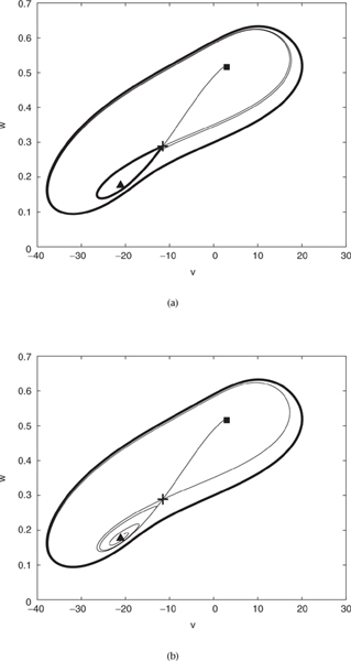
Figure 5.20 Phase portraits of the Morris-Lecar system close to a homoclinic orbit. (a) and (c) = 0.202553 (b) and (d) = 0.202554.

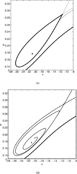
Figure 5.20 (continued) The phase portraits (c) and (d) show an expanded view of those in figures (a) and (b). Observe carefully the relative position of the stable and unstable manifolds of the saddle in (c) and (d).

Figure 5.21 Bifurcation curves of saddle-node (vertical) and Hopf bifurcation (curved) in the plane of the parameters (g_Ca, ). The curves intersect tangentially at the end point of the Hopf bifurcation curve, a Takens-Bogdanov point.

More complicated bifurcations than the ones described above can be expected to be found in a two-dimensional vector field with more than a single active parameter. The bifurcations encountered in generic systems with k active parameters are called codimension-k bifurcations. As k increases, the classification of codimension-k bifurcations becomes increasingly difficult. Even for two-dimensional vector fields, the largest value of k for which the classification is reasonably complete is k = 3. We give here two examples of codimension-2 bifurcations in the Morris-Lecar system. When both and g_Ca are varied at the same time, we can find parameter values for which 0 is the only eigenvalue of the Jacobian at an equilibrium point. These parameter values satisfy the defining equations for both saddle-node and Hopf bifurcations. Using Maple, we compute an approximate set of parameters for which this happens: (g_Ca, ) ≈ (5.6392, 0.2876). See Figure 5.21. This codimension-2 bifurcation is called a Takens-Bogdanov bifurcation, after the two mathematicians who first studied the properties of these bifurcations around 1970 (Guckenheimer and Holmes, 1983). Three of the bifurcations we have studied in the Morris-Lecar model—saddle nodes, Hopf bifurcation, and homoclinic bifurcation—come together at the Takens-Bogdanov bifurcation. The curve of homoclinic bifurcations lies above the curve of Hopf bifurcations in Figure 5.21, but is more difficult to compute. Figure 5.22 shows a phase portrait with (g_Ca, ) = (5.638, 0.276), parameters near the Takens-Bogdanov parameter values. This phase portrait has three equilibrium points, two of which are close together, and two periodic orbits, one of which is small. Figure 5.22b shows more detail of the region around the two nearby equilibrium points. One of the aspects of the Takens-Bogdanov bifurcation, evident in this figure, is that the eigenvectors of the saddle lie almost in the same direction. As the parameter is decreased or g_Ca is increased, the small unstable periodic orbit shrinks, meeting the equilibrium point at a subcritical Hopf bifurcation. As is increased or g_Ca is decreased, the small unstable periodic orbit becomes a homoclinic orbit and then disappears. When the parameter g_Ca increases, the two nearby equilibrium points coalesce with one another in a saddle-node bifurcation.

Figure 5.22 Phase portraits of the Morris-Lecar system close to a Takens-Bogdanov codimension-2 bifurcation. (a) There are three equilibrium points (a stable focus, a saddle and an unstable focus) and two periodic orbits. The small periodic orbit is not visible here, but can be seen in the small scale plot (b) of the phase portrait near the two lower equilibrium points.

A second type of codimension-2 bifurcation is the cusp. This bifurcation occurs in two-dimensional vector fields when the nullclines intersect with a third-order tangency, like the tangent line to a function at a point of inflection. The parameters that give the saddle-node bifurcation in Figure 5.9a appear to be close to such a point of tangency. We let i be a second active parameter with g_Ca and then find a cusp point near (g_Ca, i) = (4.97, 107.1). A pair of saddle-node curves emanate from the cusp in the parameter plane. Figure 5.23 shows the nullcline for the cusp values of the parameters along side a plot of the saddle-node curve in the (g_Ca, i) parameter plane.

5.7 Numerical Methods

Throughout the past two chapters, we have assumed that we have computer algorithms that reliably determine trajectories with specified initial conditions. This assumption is a good one, but there are pitfalls that must be avoided to obtain reliable results. Since the Morris-Lecar equations cannot be “solved” by finding explicit analytic formulas that express the trajectories as elementary functions, numerical methods that compute approximate solutions proceed step by step in time. There are many methods for solving these initial value problems. The results can vary substantially as we switch from one algorithm to another and as we change algorithmic parameters, so we discuss the fundamental ideas employed in a few of the simplest numerical methods and display some of their shortcomings. We begin with the simplest method of all, called the (explicit) Euler method.

Figure 5.23 (a) Nullclines of the Morris-Lecar system at a cusp point. The two nullclines intersect at a single point to third order. The parameters are as in Table 5.1 except that (g_Ca, i) = (4.9666, 107.06655). The location of the cusp point is independent of the parameter . (b) The saddle-node curve in the (g_Ca, i) parameter plane. The cusp bifurcation parameters are at the cusp of the saddle-node curve in this parameter plane.

In calculus, we learn that the derivative of a function gives the slope of its best linear approximations. If g(x) is a differentiable function and Δx = x – a, then the residual r(x) = g(x) – (g(a) + g′(a)(Δx)) has the property that r(x)/(Δx) → 0 as Δx → 0. For x close to a, g(a) + g′(a)(Δx) gives a good approximation to g(x). The same thing is true for solutions of the system of differential equations . If x(t) is the trajectory with x(t₀) = x₀, then x(t₀ + h) is well approximated by x₀ + hf(x₀) when the time increment h = t – t₀ is small. The line traced by x₀ + hf(x₀) as h varies is the one that the trajectory would follow if the vector field were constant, with the same value f(x₀) everywhere. Since the vector fields we study are not constant, we fix a (small) positive value of h and use x₁ = x₀ + hf(x₀) as an approximation to the point we reach on the trajectory at time t₁ = t₀ + h. We then take another step to time t₂ = t₁ + h and position x₂ = x₁ + hf(x₁). We continue in this fashion, using the iteration t_n+1 = t_n + h and x_n+1 = x_n + hf(x_n) to determine x_n+1, t_n+1 from x_n, t_n. To compute an approximation to x(T),we pick a time-step h = (T – t₀)/N for some integer N, and use N steps of this iteration. This is the Euler method. At each step, the Euler method makes an error that shrinks as h → 0. We hope that, as h → 0, the method will give values that converge to x(T). Since the number of steps grows as the step length h gets smaller, it is not evident whether we obtain this convergence or how good the approximation is. To study the approximations further, let us look at an example where we can derive formulas for the values of x(T) and and the points produced by the Euler method.

Example.

Consider the equation . From calculus, we know that the solutions to this equation are x(t) = x(0)e^t. Take T = 1 and x(0) = 1. Then x(T) = e ≈ 2.718281828 and we want to see how the values calculated by the Euler method vary when we use N steps of length h = 1/N starting at x₀ = 1. We compute the first three steps of the method to be x₁ = 1 + h, x₂ = x₁ + hx₁ = (1 + h)x₁ = (1 + h)², and x₃ = x₂ + hx₂ = (1 + h)x₂ = (1 + h)³. Continuing, we obtain x_N = (1 + h)^N = (1 + 1/N)^N. Now (1 + 1/N)^N → e as N → 0, but it does so quite slowly. Table 5.2 gives some data for this example, showing values obtained by the Euler method when N is a power of 10. The table indicates that ten thousand time-steps are required to obtain four digits of accuracy on this simple equation, a very poor performance. We also observe that each additional digit of accuracy requires about ten times the number of time-steps. In contrast to this method of calculating e and the solution to the differential equation , consider the Taylor series for

10	2.593742460
100	2.704813829
1000	2.716923932
10000	2.718145927
100000	2.718268237
1000000	2.718280469

Table 5.2 Approximate values for e obtained from the Euler method. The first column gives the number of time steps, the second column, the approximate value of e ≈ 2.718281828.

If we truncate this series after eleven terms (the last term we give has n = 10), it gives an approximate value of e as 2.718281801. Extrapolating from our observations about the Euler method, comparable accuracy would require roughly 100 million time steps! Thus the Euler method is a very poor way of obtaining highly accurate approximations to solutions of differential equations. We want methods that require fewer calculations to achieve a given accuracy.

One path to finding more accurate numerical methods for solving ordinary differential equations is to focus upon the order of the numerical methods. The order is defined by the relationship between the step length h and the error the method makes in computing x(t + h) from x(t). If the error in computing one step is proportional to h^d+1, then the method has order d. When we use N steps of length h = T/N to compute an approximate solution at time t₀ + T, N = T/h has order 1/h. Thus, the error of a method of order d in computing x(T) tends to zero as h^d as h → 0.

In our example of computing e by solving the differential equation , replacing the Euler method by the degree d truncation of the Taylor series of the exponential function gives increasingly accurate order-d approximations to the solution. For example, a single step of length 1 with d = 10 gives two more digits of accuracy than a million steps of the Euler method. Even “low”-degree methods give an enormous improvement: ten steps of length 1/10 with d = 4 give a value of 2.718279744, with accuracy comparable to the Euler method with a million steps.

There are varied approaches to the construction of higher-order methods for solving differential equations. We mention two, one to illustrate the principle and the second because it is frequently used. The second-order Heun’s method has time-step map H_h(x) = x + (h/2)(f(x) + f(x + hf(x))). Note that producing each time-step requires evaluating f twice, once at x and once at x + hf(x). To see that the method has second order, we first compute the Taylor expansion of H_h(x) in h, obtaining x + f(x)h + f′(x)f(x)h². Next we differentiate the equation with respect to t, to get using the chain rule. These equations imply that the degree-1 and -2 terms of the Taylor expansion of x(t) have coefficients f(x) and f′(x)f(x), agreeing with the Taylor expansion of Heun’s method. Similar, but longer, calculations lead to still higher-order methods. For example, the Runge-Kutta method with time-step map R_h defined by

has fourth order. When accuracy of a numerical simulation is important, use higher-order methods if at all possible.

In addition to accuracy, the stability of numerical methods for solving initial value problems is also important. To illustrate the issue, consider Euler’s method applied to the equation with a > 0 large. The solution of this equation with x(0) = x₀ is x(t) = e^–atx₀. As t → ∞, the solution approaches 0 very, very quickly. The time-step map from the Euler method is E_h(x) = x(1 – ah). N iterations of E_h send x to x(1 – ah)^N .If ah > 2, then |1 – ah| > 1 and |1 – ah|^N increases geometrically with N. Thus the behavior of the iterates of E_h is completely different from that of the solution of the differential equation. Instead of monotonically approaching 0, the iterates of E_h increase in magnitude with alternating signs. To avoid this unstable behavior of the numerical integration, the time-step is limited by ah < 2. If 1 < ah < 2, the iterates of E_h approach 0, but they oscillate in sign as they do so.

Constraints on the time-step h of a method are a big issue in applications of biological interest. If time-steps are limited by the fastest rates of exponential decay in a system, then we will have difficulty working with models that include fast processes that quickly approach equilibrium. The model for enzyme kinetics introduced in Chapter 1 is already an example of this phenomenon. Simulations of the three-dimensional motions of proteins provide a somewhat different challenge in handling multiple time scales in systems of differential equations. The frequencies of oscillations in individual bonds within a molecule are many orders of magnitude faster than the time required for the folding of the molecule. Attempts to predict three-dimensional structure from simulation of the molecular dynamics must encompass this range of time scales, a task that is still not feasible on today’s fastest computers. Within the numerical analysis literature, systems with multiple time scales are called stiff. Numerical methods have been created for integrating stiff systems. The simplest of these is the implicit Euler method.

Implicit methods require that one solves a system of equations to determine the point at the end of a step. The simplest example is the implicit Euler method defined by the equations I_h(x) = x + hf(I_h(x)). To determine I_h(x), we need to solve these equations at each step. Newton’s method is typically used to find the solution. As before, we can analyze the method completely for the linear equation . The equation to be solved is I_h(x) = x – haI_h(x) whose solution is I_h(x) = x/(1 + ah). This implies that after n steps, x is mapped to x/(1 + ah)ⁿ.As n increases, this tends to 0 in a monotone way for all a, h > 0. Thus the method avoids the instability and step length limitations of the explicit Euler method. In a stiff system, we can usually use step lengths based upon the slower time scales in the system without causing instability due to rapidly decaying components of a solution. Even though the implicit Euler method is more stable than the explicit Euler method, it still has first order. The second-degree Taylor expansion of x/(1 + ah) in h is x(1 − ah + a²h² – . . .) = x − ahx + a²h²x − . . . . The second-degree term in the Taylor expansion of e^–ahx is , not a²x, so the method is only first-order accurate. In general, implicit methods are slower than explicit methods when used with the same step size due to the time required to solve the implicit equations. Their advantage is that it is often possible to take much larger steps and still maintain stability.

The limitations on step size associated with accuracy and instability may change substantially along a trajectory. To deal with this, it is common practice to use methods that change step sizes during the calculation of trajectories. Procedures have been developed for estimating the error of a tentative step and adjusting the step length based upon this information. The simplest procedure is to do the following. If the estimated error exceeds a desired threshold, then a smaller step is chosen. If the estimated error is smaller than a lower threshold, then a larger step is attempted. The effect of such a strategy is to utilize the largest step sizes that are consistent with specified error tolerances. In practice, the additional computational cost in estimating error tolerances is more than offset by the smaller number of steps required to compute trajectories. On occasion, the step length selection procedures can be overly optimistic and give results that do become unstable.

We depend upon thoroughly tested computer algorithms to solve solutions to initial value problems for systems of differential equations, just as we depend upon algorithms to compute eigenvalues and eigenvectors of matrices. However, there is a wider range of performance and more choices to be made in solving differential equations. There are three things to keep in mind when using numerical integration:

• It is easy to get spurious results by misusing an algorithm. So be skeptical and check your results, for example by using more than one step size to solve the same problem, and by comparing solutions to the same problem computed with different methods.

• There are problems, like molecular simulations of protein folding, that remain beyond the capability of current methods. Be realistic in your expectations of what computers can do, and creative in dealing with problems that seem beyond the pale.

• There is a mathematical framework that is helpful in developing a consistent interpretation of simulation results. If numerical results appear to be at odds with the theory, work to resolve the discrepancies.

5.8 Summary

This chapter is the most mathematical in this book. Nonetheless, it gives only a brief introduction to dynamical systems theory. Systems of ordinary differential equations are perhaps the most common type of dynamic models in all of the sciences, so it is worthwhile to learn how to work with them. That is a task that involves lots of computation and lots of mathematics. The language that has been developed to describe the patterns formed by these systems and the logic of concentrating attention on generic systems can be intimidating when we first encounter them. As with most skills, proficiency with this type of analysis comes with experience and practice. We have used a single example, the Morris-Lecar model, to illustrate phenomena described in much greater generality by the theory. We hope that you will explore additional examples of differential equation models with complex dynamics and study the mathematics in more depth so that you can use it with confidence as a tool in your explorations.

The next chapter applies what we have learned here to differential equation models of infectious disease. In the simplest of these models, analytical techniques take us a long way and the dynamics are simpler than those of the Morris-Lecar model. However, sustained oscillations of childhood endemic diseases like chicken pox and measles have been observed, and we will use dynamic models to gain insight into the causes of these oscillations. Subsequent chapters will consider still more complex dynamic models of biological systems where the mathematical foundations for interpreting the model results are weaker than is the case for ordinary differential equations.

5.9 References

Blanchard, P., R. Devaney, and G. Hall. 2002. Differential Equations, 2nd edition. Brooks/Cole.

Guckenheimer, J., and P. Holmes. 1983. Nonlinear Oscillations, Dynamical Systems, and Bifurcation of Vector Fields. Springer-Verlag.

Hirsch, M. W., S. Smale, and R. L. Devaney. 2004. Differential Equations, Dynamical Systems, and an Introduction to Chaos. Elsevier, Amsterdam.

Rinzel J. and B. Ermentrout. 1998. Analysis of neural excitability and oscillations. Pages 251–292 in C. Koch and I. Seger (eds), Methods in Neuronal Modeling. MIT Press, Cambridge.

Strogatz, S. 1994. Nonlinear Dynamics and Chaos: With Applications to Physics, Biology, Chemistry and Engineering. Perseus Publishing.

¹The equations [5.4] are called autonomous because the functions f do not depend upon t. One can study nonautonomous equations in which the f may depend upon t, but the geometric interpretations of their solutions are more complicated.

²The terms vector and point are sometimes used interchangeably and sometimes in distinct ways. When both refer to x, we call f(f) a tangent vector to distinguish it from x. Some authors call the quantities x points and the quantities f(f) vectors. We have tried to avoid confusion by making minimal use of the term vector to describe either x or f (x).

³The smallest number larger than 1 that can be represented in “double-precision” floating-point arithmetic is approximately 1 + 10^–16.

⁴This statement is proved by studying the index of a vector field along closed curves. The index of the vector field on a curve without equilibrium points measures the number of times that the vector field rotates around the origin while traversing the curve.

⁵Some systems have continuous families of periodic orbits, something that is impossible to verify rigorously by numerical integration.

⁶The two parameters that differ between the two sets are g_Ca and . Experimentally, g_Ca can be reduced with substances that block calcium channels, while changes with temperature.

⁷The implicit function theorem implies that an equilibrium with no zero eigenvalues varies smoothly with respect to parameters. The determinant of a matrix is the product of the eigenvalues, so a defining equation for a saddle-node bifurcation is that the determinant of the Jacobian vanishes. Notice that the curve of equilibria in (x, μ) space is a smooth parabola, defined by μ + x² = 0. However, at the bifurcation, we cannot solve for the equilibrium point as a function of the parameters. Numerical continuation methods designed to track the curve of equilibria follow the curve around its “turning point” rather than incrementing the parameter and searching for equilibrium points at each fixed parameter value.

⁸A similar phenomenon happens at some saddle-node bifurcations of an equilibrium. After the equilibria disappear at the bifurcation, a periodic orbit that passes through the region where the equilibrium points were located may appear. The term snic (saddle node on invariant circle) was used by Rinzel and Ermentrout to describe these saddle-node bifurcations.