22.10.1 AABB

Assume we have an AABB, B, defined by a center point, c , and a positive half diagonal vector, h . Note that c and h can easily be derived from the minimum and maximum corners, b min and b max of B, that is, c = ( b max + b min ) / 2 , and h = ( b max - b min ) / 2 .

Now, we want to test B against a plane n · x + d = 0 . There is a surprisingly fast way of performing this test. The idea is to compute the “extent,” here denoted e, of the box when projected onto the plane normal, n . In theory, this can be done by projecting all the eight different half diagonals of the box onto the normal, and picking the longest one. In practice, however, this can be implemented rapidly as

Why is this equivalent to finding the maximum of the eight different half diagonals projections? These eight half diagonals are the combinations: g i = ( ± h x , ± h y , ± h z ) , and we want to compute g i · n for all eight i. The dot product g i · n will reach its maximum when each term in the dot product is positive. For the x-term, this will happen when n x has the same sign as h x i , but since we know that h x is positive already, we can compute the max term as h x | n x | . Doing this for y and z as well gives us Equation 22.18.

Next, we compute the signed distance, s, from the center point, c , to the plane. This is done with: s = c · n + d . Both s and e are illustrated in Figure 22.18. Assuming that the “outside” of the plane is the positive half-space, we can simply test if s - e > 0 , which then indicates that the box is fully outside the plane. Similarly, s + e < 0 indicates that the box is fully inside. Otherwise, the box intersects the plane. This technique is based on ideas by Ville Miettinen and his clever implementation. Pseudocode is below:

22.10.2. OBB

Testing an OBB against a plane differs only slightly from the AABB/plane test from the previous section. It is only the computation of the “extent” of the box that needs to be changed, which is done as

Recall that ( b u , b v , b w ) are the coordinate system axes (see the definition of the OBB in Section 22.2) of the OBB, and ( h u B , h v B , h w B ) are the lengths of the box along these axes.

22.11 Triangle/Triangle Intersection

Since graphics hardware uses the triangle as its most important (and optimized) drawing primitive, it is only natural to perform collision detection tests on this kind of data as well. So, the deepest levels of a collision detection algorithm typically have a routine that determines whether or not two triangles intersect. Given two triangles, T 1 = ▵ p 1 p 2 p 3 and T 2 = ▵ q 1 q 2 q 3 (which lie in the planes π 1 and π 2 , respectively), we want to determine whether or not they intersect.

From a high level, it is common to start by checking whether T 1 intersects with π 2 , and whether T 2 intersects with π 1 [1232]. If either of these tests fails, there can be no intersection. Assuming the triangles are not coplanar, we know that the intersection of the planes, π 1 and π 2 , will be a line, L. This is illustrated in Figure 22.19. From the figure, it can be concluded that if the triangles intersect, their intersections on L will also have to overlap. Otherwise, there will be no intersection. There are different ways to implement this, and we present the method by Guigue and Devillers [622] next.

In this implementation, there is heavy use of 4 × 4 determinants from four three-dimensional vectors, a , b , c , and d :

Geometrically, Equation 22.20 has an intuitive interpretation. The cross product, ( b - a ) × ( c - a ) , can be seen as computing the normal of a triangle, Δ a b c . By taking the dot product between this normal and the vector from a to d , we get a value that is positive if d is in the positive half-space of the triangle’s plane, Δ a b c . An alternative interpretation is that the sign of the determinant tells us whether a screw in the direction of b - a turns in the same direction as indicated by d - c . This is illustrated in Figure 22.20.

We first test whether T 1 intersects with π 2 , and vice versa. This can be done using the specialized determinants from Equation 22.20 by evaluating [ q 1 , q 2 , q 3 , p 1 ] , [ q 1 , q 2 , q 3 , p 2 ] , and [ q 1 , q 2 , q 3 , p 3 ] . The first test is equivalent to computing the normal of T 2 , and then testing which half-space the point p 1 is in. If the signs of these determinants are the same and nonzero, there can be no intersection, and the test ends. If all are zero, the triangles are coplanar, and a separate test is performed to handle this case. Otherwise, we continue testing whether T 2 intersects with π 1 , using the same type of test.

At this point, two intervals, I 1 = [ i , j ] and I 2 = [ k , l ] , on L are to be computed, where I 1 is computed from T 1 and I 2 from T 2 . To do this, the vertices for each triangle are reordered so the first vertex is alone on one side of the other triangle’s plane. If I 1 overlaps with I 2 , then the two triangles intersect, and this occurs only if k ≤ j and i ≤ l . To implement k ≤ j , we can use the sign test of the determinant (Equation 22.20), and note that j is derived from p 1 p 2 , and k from q 1 q 2 . Using the interpretation of the “screw test” of the determinant computation, we can conclude that k ≤ j if [ p 1 , p 2 , q 1 , q 2 ] ≤ 0 . The final test then becomes

The entire test starts with six determinant tests, and the first three share the first arguments, so many computations can be shared. In principle, the determinant can be computed using many smaller 2 × 2 subdeterminants, and when these occur in more than one 4 × 4 determinant, the computations can be shared. There is code on the web for this test [622], and it is also possible to augment the code to compute the actual line segment of intersection.

If the triangles are coplanar, they are projected onto the axis-aligned plane where the areas of the triangles are maximized (Section 22.9). Then, a simple two-dimensional triangle-triangle overlap test is performed. First, test all closed edges (i.e., including endpoints) of T 1 for intersection with the closed edges of T 2 . If any intersection is found, the triangles intersect. Otherwise, we must test whether T 1 is entirely contained in T 2 or vice versa. This can be done by performing a point-in-triangle test (Section 22.8) for one vertex of T 1 against T 2 , and vice versa.

Note that the separating axis test (see page 947) can be used to derive a triangle/triangle overlap test. We instead presented a test by Guigue and Devillers [622], which is faster than using SAT. Other algorithms exist for performing triangle/triangle intersection [713,1619,1787] as well. Architectural and compiler differences, as well as variation in expected hit ratios, mean that we cannot recommend a single algorithm that always performs best. Note that precision problems can occur as with any geometrical tests. Robbins and Whitesides [1501] use the exact arithmetic by Shewchuk [1624] to avoid this.

22.12 Triangle/Box Intersection

This section presents an algorithm for determining whether a triangle intersects an axis-aligned box. Such a test is useful for voxelization and for collision detection.

Green and Hatch [581] present an algorithm that can determine whether an arbitrary polygon overlaps a box. Akenine-Möller [21] developed a faster method that is based on the separating axis test (page 947), and which we present here. Triangle/sphere testing can also be performed using this test, see Ericson’s article [440] for details.

We focus on testing an axis-aligned bounding box (AABB), defined by a center c , and a vector of half lengths, h , against a triangle Δ u 0 u 1 u 2 . To simplify the tests, we first move the box and the triangle so that the box is centered around the origin, i.e., v i = u i - c , i ∈ { 0 , 1 , 2 } . This translation and the notation used is shown in Figure 22.21. To test against an oriented box, we would first rotate the triangle vertices by the inverse box transform, then use the test here. Based on the separating axis test (SAT), we test the following 13 axes:

1. [3 tests] e 0 = ( 1 , 0 , 0 ) , e 1 = ( 0 , 1 , 0 ) , e 2 = ( 0 , 0 , 1 ) (the normals of the AABB). In other words, test the AABB against the minimal AABB around the triangle.
2. [1 test] n , the normal of Δ u 0 u 1 u 2 . We use a fast plane/AABB overlap test (Section 22.10.1), which tests only the two vertices of the box diagonal whose direction is most closely aligned to the normal of the triangle.
3. [9 tests] a ij = e i × f j , i , j ∈ { 0 , 1 , 2 } , where f 0 = v 1 - v 0 , f 1 = v 2 - v 1 , and f 2 = v 0 - v 2 , i.e., edge vectors. These tests are similar in form and we will only show the derivation of the case where i = 0 and j = 0 (see below).

As soon as a separating axis is found the algorithm terminates and returns “no overlap.” If all tests pass, i.e., there is no separating axis, then the triangle overlaps the box.

Here we derive one of the nine tests, where i = 0 and j = 0 , in Step 3. This means that a 00 = e 0 × f 0 = ( 0 , - f 0 z , f 0 y ) . So, now we need to project the triangle vertices onto a 00 (hereafter called a ):

Normally, we would have had to find min ( p 0 , p 1 , p 2 ) and max ( p 0 , p 1 , p 2 ) , but fortunately p 0 = p 1 , which simplifies the computations. Now we only need to find min ( p 0 , p 2 ) and max ( p 0 , p 2 ) , which is significantly faster because conditional statements are expensive on modern CPUs.

After the projection of the triangle onto a , we need to project the box onto a as well. We compute a “radius,” r, of the box projected on a as

where the last step comes from that a x = 0 for this particular axis. Then, this axis test becomes

Code is available on the web [21].

22.13 Bounding-Volume/Bounding-Volume Intersection

The purpose of a bounding volume is to provide simpler intersection tests and make more efficient rejections. For example, to test whether or not two cars collide, first find their BVs and test if these overlap. If they do not, then the cars are guaranteed not to collide (which we assume is the most common case). We then have avoided testing each primitive of one car against each primitive of the other, thereby saving computation.

A fundamental operation is to test whether or not two bounding volumes overlap. Methods of testing overlap for the AABB, the k-DOP, and the OBB are presented in the following sections. See Section 22.3 for algorithms that form BVs around primitives.

The reason for using more complex BVs than the sphere and the AABB is that more complex BVs often have a tighter fit. This is illustrated in Figure 22.22. Other bounding volumes are possible, of course. For example, cylinders and ellipsoids are sometimes used as bounding volumes for objects. Also, several spheres can be placed to enclose a single object [782,1582].

For capsule and lozenge BVs it is a relatively quick operation to compute the minimum distance. Therefore, they are often used in tolerance verification applications, where one wants to verify that two (or more) objects are at least a certain distance apart. Eberly [404] and Larsen et al. [979] derive formulae and efficient algorithms for these types of bounding volumes.

22.13.1. Sphere/Sphere Intersection

For spheres, the intersection test is simple and quick: Compute the distance between the two spheres’ centers and then reject if this distance is greater than the sum of the two spheres’ radii. Otherwise, they intersect. In implementing this algorithm, it is best to use the squared distances of these two quantities, since all that is desired is the result of the comparison. In this way, computing the square root (an expensive operation) is avoided. Ericson [435] gives SSE code for testing four separate pairs of spheres simultaneously.

22.13.2. Sphere/Box Intersection

An algorithm for testing whether a sphere and an AABB intersect was first presented by Arvo [70] and is surprisingly simple. The idea is to find the point on the AABB that is closest to the sphere’s center, c . One-dimensional tests are used, one for each of the three axes of the AABB. The sphere’s center coordinate for an axis is tested against the bounds of the AABB. If it is outside the bounds, the distance between the sphere center and the box along this axis (a subtraction) is computed and squared. After we have done this along the three axes, the sum of these squared distances is compared to the squared radius, r 2 , of the sphere. If the sum is less than the squared radius, the closest point is inside the sphere, and the box overlaps. As Arvo shows, this algorithm can be modified to handle hollow boxes and spheres, as well as axis-aligned ellipsoids.

Larsson et al. [982] present some variants of this algorithm, including a considerably faster SSE vectorized version. Their insight is to use simple rejection tests early on, either per axis or all at the start. The rejection test is to see if the center-to-box distance along an axis is greater than the radius. If so, testing can end early, since the sphere then cannot possibly overlap with the box. When the chance of overlap is low, this early rejection method is noticeably faster. What follows is the QRI (quick rejections intertwined) version of their test. The early out tests are at lines 4 and 7, and can be removed if desired.

For a fast vectorized (using SSE) implementation, Larsson et al. propose to eliminate most of the branches. The idea is to evaluate lines 3 and 6 simultaneously using the following expression:

Normally, we would then update d as d = d + e 2 . However, using SSE, we can evaluate Equation 22.25 for x, y, and z in parallel. Pseudocode for the full test is given below.

Note that lines 1 and 2 can be implemented using a parallel SSE max function. Even though there are no early outs in this test, it is still faster than the other techniques. This is because branches have been eliminated and parallel computations used. Another approach to SSE is to vectorize the object pairs. Ericson [435] presents SIMD code to compare four spheres with four AABBs at the same time.

For sphere/OBB intersection, first transform the sphere’s center into the OBB’s space. That is, use the OBB’s normalized axes as the basis for transforming the sphere’s center. Now this center point is expressed relative to the OBB’s axes, so the OBB can be treated as an AABB. The sphere/AABB algorithm is then used to test for intersection.

Larsson [983] gives an efficient method for ellipsoid/OBB intersection testing. First, both objects are scaled so that the ellipsoid becomes a sphere and the OBB a parallelepiped. Sphere/slab intersection testing can be performed for quick acceptance and rejection. Finally, the sphere is tested for intersection with only those parallelograms facing it.

22.13.3. AABB/AABB Intersection

An AABB is, as its name implies, a box whose faces are aligned with the main axis directions. Therefore, two points are sufficient to describe such a volume. Here we use the definition of the AABB presented in Section 22.2.

Due to their simplicity, AABBs are commonly employed both in collision detection algorithms and as bounding volumes for the nodes in a scene graph. The test for intersection between two AABBs, A and B, is trivial and is summarized below:

Lines 1 and 2 loop over all three standard axis directions x, y, and z. Ericson [435] provides SSE code for testing four separate pairs of AABBs simultaneously.

22.13.4. k-DOP/k-DOP Intersection

The intersection test for a k-DOP with another k-DOP consists of only k / 2 interval overlap tests. Klosowski et al. [910] have shown that, for moderate values of k, the overlap test for two k-DOPs is an order of magnitude faster than the test for two OBBs. In Figure 22.4 on page 946, a simple two-dimensional k-DOP is depicted. Note that the AABB is a special case of a 6-DOP where the normals are the positive and negative main axis directions. OBBs are also a form of 6-DOP, but this fast test can be used only when the two OBBs share the same axes.

The intersection test that follows is simple and extremely fast, inexact but conservative. If two k-DOPs, A and B (superscripted with indices A and B), are to be tested for intersection, then test all parallel pairs of slabs ( S i A , S i B ) for overlap; s i = S i A ∩ S i B is a one-dimensional interval overlap test, which is solved with ease. This is an example of dimension reduction, as the rules of thumb in Section 22.5 recommend. Here, a three-dimensional slab test is simplified into a one-dimensional interval overlap test.

If at any time s i = ∅ (i.e., the empty set), then the BVs are disjoint and the test is terminated. Otherwise, the slab overlap tests continues. If and only if all s i ≠ ∅ , 1 ≤ i ≤ k / 2 , then the BVs are considered overlapping. According to the separating axis test (Section 22.2), one also needs to test an axis parallel to the cross product of one edge from each k-DOP. However, these tests are often omitted because they cost more than they give back in performance. Therefore, if the test below returns that the k-DOPs overlap, then they might actually be disjoint. Here is the pseudocode for the k-DOP/k-DOP overlap test:

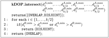
Note that only k scalar values need to be stored with each instance of the k-DOP (the normals, n i , are stored once for all k-DOPs since they are static). If the k-DOPs are translated by t A and t B , respectively, the test gets a tiny bit more complicated. Project t A onto the normals, n i , e.g., p i A = t A · n i (note that this is independent of any k-DOP and therefore needs to be computed only once for each t A or t B ) and add p i A to d i A , min and d i A , max in the if-statement. The same is done for t B . In other words, a translation changes the distance of the k-DOP along each normal’s direction.

Laine and Karras [965] present an extension to k-DOPs called the apex point map. The idea is to map a set of plane normals to various points on the k-DOP, such that each point stored represents the most distant location along that direction. This point and the direction form a plane that fully contains the model in one half-space, i.e., the point is at the apex of the model’s k-DOP. During testing, the apex point retrieved for a given direction can be used for a more accurate intersection test between k-DOPs, for improved frustum culling, and for finding tighter AABBs after rotation, as some examples.

22.13.5. OBB/OBB Intersection

In this section we briefly outline a fast method for testing intersection between two OBBs, A and B [436,576,577]. The algorithm uses the separating axis test, and is about an order of magnitude faster than previous methods, which use closest features or linear programming. The definition of the OBB may be found in Section 22.2.

The test is done in the coordinate system formed by A’s center and axes. This means that the origin is a c = ( 0 , 0 , 0 ) and that the main axes in this coordinate system are a u = ( 1 , 0 , 0 ) , a v = ( 0 , 1 , 0 ) , and a w = ( 0 , 0 , 1 ) . Moreover, B is assumed to be located relative to A, with a translation t and a rotation (matrix) R .

According to the separating axis test, it is sufficient to find one axis that separates A and B to be sure that they are disjoint (do not overlap). Fifteen axes have to be tested: three from the faces of A, three from the faces of B, and 3 · 3 = 9 from combinations of edges from A and B. This is shown in two dimensions in Figure 22.23. As a consequence of the orthonormality of the matrix A = ( a u a v a w ) , the potential separating axes that should be orthogonal to the faces of A are simply the axes a u , a v , and a w . The same holds for B. The remaining nine potential axes, formed by one edge each from both A and B, are then c ij = a i × b j , ∀ i ∈ { u , v , w } and ∀ j ∈ { u , v , w } . Luckily, there is optimized code online for this [1574].

22.14 View Frustum Intersection

As has been seen in Section 19.4, hierarchical view frustum culling is essential for rapid rendering of a complex scene. One of the few operations called during bounding-volume-hierarchy cull traversal is the intersection test between the view frustum and a bounding volume. These operations are thus critical to fast execution. Ideally, they should determine whether the BV is fully inside (inclusion), it is entirely outside (exclusion), or it intersects the frustum.

To review, a view frustum is a pyramid that is truncated by a near and a far plane (which are parallel), making the volume finite. In fact, it becomes a polyhedron. This is shown in Figure 22.24, where the names of the six planes, near, far, left, right, top, and bottom also are marked. The view frustum volume defines the parts of the scene that should be visible and thus rendered (in perspective for a pyramidal frustum).

The most common bounding volumes used for internal nodes in a hierarchy (e.g., a scene graph) and for enclosing geometry are spheres, AABBs, and OBBs. Therefore frustum/sphere and frustum/AABB/OBB tests will be discussed and derived here.

To see why we need the three return results outside/inside/intersect, we will examine what happens when traversing the bounding volume hierarchy. If a BV is found to be entirely outside the view frustum, then that BV’s subtree will not be traversed further and none of its geometry will be rendered. On the other hand, if the BV is fully inside, then no more frustum/BV tests need to be computed for that subtree and every renderable leaf will be drawn. For a partially visible BV, i.e., one that intersects the frustum, the BV’s subtree is tested recursively against the frustum. If the BV is for a leaf, then that leaf must be rendered.

The complete test is called an exclusion/inclusion/intersection test. Sometimes the third state, intersection, may be considered too costly to compute. In this case, the BV is classified as “probably inside.” We call such a simplified algorithm an exclusion/inclusion test. If a BV cannot be excluded successfully, there are two choices. One is to treat the “probably inside” state as an inclusion, meaning that everything inside the BV is rendered. This is often inefficient, as no further culling is performed. The other choice is to test each node in the subtree in turn for exclusion. Such testing is often without benefit, as much of the subtree may indeed be inside the frustum. Because neither choice is particularly good, some attempt at quickly differentiating between intersection and inclusion is often worthwhile, even if the test is imperfect.

It is important to realize that the quick classification tests do not have to be exact for scene-graph culling, just conservative. For differentiating exclusion from inclusion, all that is required is that the test err on the side of inclusion. That is, objects that should actually be excluded can erroneously be included. Such mistakes simply cost extra time. On the other hand, objects that should be included should never be quickly classified as excluded by the tests, otherwise rendering errors will occur. With inclusion versus intersection, either type of incorrect classification is usually legal. If a fully included BV is classified as intersecting, time is wasted testing its subtree for intersection. If an intersected BV is considered fully inside, time is wasted by rendering all objects, some of which could have been culled.

Before we introduce the tests between a frustum and a sphere, AABB, or OBB, we shall describe an intersection test method between a frustum and a general object. This test is illustrated in Figure 22.25. The idea is to transform the test from a BV/frustum test to a point/volume test. First, a point relative to the BV is selected. Then the BV is moved along the outside of the frustum, as closely as possible to it without overlapping. During this movement, the point relative to the BV is traced, and its trace forms a new volume (a polygon with thick edges in Figure 22.25). The fact that the BV was moved as close as possible to the frustum means that if the point relative to the BV (in its original position) lies inside the traced-out volume, then the BV intersects or is inside the frustum. So, instead of testing the BV for intersection against a frustum, the point relative to the BV is tested against another new volume, which is traced out by the point. In the same way, the BV can be moved along the inside of the frustum and as close as possible to the frustum. This will trace out a new, smaller frustum with planes parallel to the original frustum [83]. If the point relative to the object is inside this new volume, then the BV is fully inside the frustum. This technique is used to derive tests in the subsequent sections. Note that the creation of the new volumes is independent of the position of the actual BV—it is dependent solely on the position of the point relative to the BV and the shape of the BV. This means that a BV with an arbitrary position can be tested against thesame volumes.

Saving just a parent BV’s intersection state with each child is a useful optimization. If the parent is known to be fully inside the frustum, none of the descendants need any further frustum testing. The plane masking and temporal coherence techniques discussed in Section can also noticeably improve testing against a bounding volume hierarchy, though are less useful with a SIMD implementation [529].

First, we derive the plane equations of the frustum, since these are needed for these sorts of tests. Frustum/sphere intersection is presented next, followed by an explanation of frustum/box intersection.

22.14.1. Frustum Plane Extraction

To do view frustum culling, the plane equations for the six different sides of the frustum are needed. We present here a clever and fast way of deriving these. Assume that the view matrix is V and that the projection matrix is P . The composite transform is then M = P V . A point s (where s w = 1 ) is transformed into t as t = M s . At this point, t may have t w ≠ 1 due to, for example, perspective projection. Therefore, all components in t are divided by t w to obtain a point u with u w = 1 . For points inside the view frustum, it holds that - 1 ≤ u i ≤ 1 , for i ∈ x , y , z , i.e., the point u is inside a unit cube. This is for the OpenGL type of projection matrices (Section ). For DirectX, the same holds, except that 0 ≤ u z ≤ 1 . The planes of the frustum can be derived directly from the rows of the composite transform matrix.

Focus for a moment on the volume on the right side of the left plane of the unit cube, for which - 1 ≤ u x . This is expanded below:

In the derivation, m i , denotes the ith row in M . The last step ( m 0 , + m 3 , ) · s ≥ 0 is, in fact, denoting a (half) plane equation of the left plane of the view frustum. This is so because the left plane in the unit cube has been transformed back to world coordinates. Also note that s w = 1 , which makes the equation a plane. To make the normal of the plane point outward from the frustum, the equation must be negated (as the original equation described the inside of the unit cube). This gives - ( m 3 , + m 0 , ) · ( x , y , z , 1 ) = 0 for the left plane of the frustum (where we use (x, y, z, 1) instead to use a plane equation of the form: a x + b y + c z + d = 0 ). To summarize, all the planes are

Code for doing this in OpenGL and DirectX is available on the web [600].

22.14.2. Frustum/Sphere Intersection

A frustum for an orthographic view is a box, so the overlap test in this case becomes a sphere/OBB intersection and can be solved using the algorithm presented in Section 22.13.2. To further test whether the sphere is entirely inside the box, we first check if the sphere’s center is between the box’s boundaries along each axis by a distance greater than its radius. If it is between these in all three dimensions, it is fully contained. For an efficient implementation of this modified algorithm, along with code, see Arvo’s article [70].

Following the method for deriving a frustum/BV test, for an arbitrary frustum we select the center of the sphere as the point p to trace. This is shown in Figure 22.26. If the sphere, with radius r, is moved along the inside and along the outside of the frustum and as close to the frustum as possible, then the trace of p gives us the volumes that are needed to reformulate the frustum/sphere test. The actual volumes are shown in the middle segment of Figure 22.26. As before, if p is outside the orange volume, then the sphere is outside the frustum. If p is inside the violet area, then the sphere is completely inside the frustum. If the point is inside the orange area, the sphere intersects the frustum sides planes. In this way, the exact test can be done. However, for the sake of efficiency we use the approximation that appears on the right side of Figure 22.26. Here, the orange volume has been extended in order to avoid the more complicated computations that the rounded corners would require. Note that the outer volume consists of the planes of the frustum moved r distance units outward in the direction of the frustum plane normal, and that the inner volume can be created by moving the planes of the frustum r distance units inward in the direction of the frustum plane normals.

Assume that the plane equations of the frustum are such that the positive half-space is located outside of the frustum. Then, an actual implementation would loop over the six planes of the frustum, and for each frustum plane, compute the signed distance from the sphere’s center to the plane. This is done by inserting the sphere center into the plane equation. If the distance is greater than the radius r, then the sphere is outside the frustum. If the distances to all six planes are less than - r , then the sphere is inside the frustum; otherwise the sphere intersects it. More correctly, we say that the sphere intersects the frustum, but the sphere center may be located in one of the sharp corner areas outside the rounded corners shown in Figure 22.26. This would mean that the sphere is outside the frustum, but we report it to be intersecting, to be conservatively correct.

To make the test more accurate, it is possible to add extra planes for testing if the sphere is outside. However, for the purposes of quickly culling out scene-graph nodes, occasional false hits simply cause unnecessary testing, not algorithm failure, and this additional testing will cost more time overall. Another more accurate, though still imprecise, method is described in Section 20.3, useful for when these sharp corner areas are significant.

For efficient shading techniques, the frusta are often highly asymmetrical and a special method for that is described in Figure 20.7 on page 895. Assarsson and Möller [83] provide a method that eliminates three planes from each test by dividing the frustum into octants and finding in which octant the center of the object is located.

22.14.3. Frustum/Box Intersection

If the view’s projection is orthographic (i.e., the frustum has a box shape), precise testing can be done using OBB/OBB intersection testing (Section 22.13.5). For general frustum/box intersection testing, there are two methods commonly used. One simple method is to transform all eight box corners to the frustum’s coordinate system by using the view and projection matrices for the frustum. Perform clip testing for the canonical view volume that extends [ - 1 , 1 ] along each axis (Section ). If all points are outside one boundary, the box is rejected; if all are in, the box is fully contained [529]. As this method emulates clipping, it can be used for any object delimited by a set of points, such as a line segment, triangle, or k-DOP. An advantage of this method is that no frustum plane extraction is needed. Its self-contained simplicity lends it to efficient use in a compute shader [1883,1884].

A method that is considerably more efficient on the CPU is to use the plane/box intersection test described in Section 22.10. Like the frustum/sphere test, the OBB or AABB is checked against the six view frustum planes. Instead of computing the signed distance of all eight corners from a plane, in the plane/box test we check at most two corners, determined by the plane’s normal. If the nearest corner is outside the plane, the box is fully outside and testing can end early. If the farthest corner for every plane is inside, then the box is contained inside the frustum. Note that the dot product distance computations for the near and far planes can be shared, since these planes are parallel. The only additional cost for this second method is that the frustum’s planes must first be derived, a trivial expense if a few boxes are tobe tested.

Like the frustum/sphere algorithm, the test suffers from classifying boxes as intersecting that are actually fully outside. Those kinds of errors are shown in Figure 22.27. Quílez [1452] notes that this can happen more frequently with fixed-size terrain meshes or other large objects. When an intersection is reported, his solution is to then also test the corners of the frustum against each of the planes forming the bounding box. If all points are outside a box’s plane, the frustum and box do not intersect. This additional test is equivalent to the second part of the separating axis test, where the axis tested is orthogonal to the second object’s faces. That said, such additional testing can be more costly than the benefits accrued. For his GIS renderer, Eng [425] found that this optimization cost 2 ms per frame of CPU time to save only a few draw calls.

Wihlidal [1884] goes the other direction with frustum culling, using only the four frustum side planes and not performing the near and far plane cull tests. He notes that these two planes do not help much in video games. The near plane is mostly redundant, since the side planes trim out almost all the space it does, and the far plane is normally set to view all objects in the scene.

Another approach is to use the separating axis test (found in Section 22.13) to derive an intersection routine. Several authors use the separating axis test for a general solution for two convex polyhedra [595,1574]. A single optimized test can then be used for any combination of line segments, triangles, AABBs, OBBs, k-DOPs, frusta, and convex polyhedra.

22.15 Line/Line Intersection

In this section, both two- and three-dimensional line/line intersection tests are derived and examined. Lines, rays, and line segments are intersected with one another, and methods that are both fast and elegant are described.

22.15.1. Two Dimensions

First Method

From a theoretical viewpoint, this first method of computing the intersection between a pair of two-dimensional lines is truly beautiful. Consider two lines, r 1 ( s ) = o 1 + s d 1 and r 2 ( t ) = o 2 + t d 2 . Since a · a ⊥ = 0 (the perp dot product [735] from Section ), the intersection calculations between r 1 ( s ) and r 2 ( t ) become elegant and simple. Note that all vectors are two-dimensional in this section:

If d 1 · d 2 ⊥ = 0 , then the lines are parallel and no intersection occurs. For lines of infinite length, all values of s and t are valid, but for line segments (with normalized directions), say of length l 1 and l 2 (starting at s = 0 and t = 0 and ending at s = l 1 and t = l 2 ), we have a valid intersection if and only if 0 ≤ s ≤ l 1 and 0 ≤ t ≤ l 2 . Or, if you set o 1 = p 1 and d 1 = p 2 - p 1 (meaning that the line segment starts at p 1 and ends at p 2 ) and do likewise for r 2 with start and end points q 1 and q 2 , then a valid intersection occurs if and only if 0 ≤ s ≤ 1 and 0 ≤ t ≤ 1 . For rays with origins, the valid range is s ≥ 0 and t ≥ 0 . The point of intersection is obtained either by plugging s into r 1 or by plugging t into r 2 .

Second Method

Antonio [61] describes another way of deciding whether two line segments (i.e., of finite length) intersect by doing more compares and early rejections and by avoiding the expensive calculations (divisions) in the previous formulae. This method is therefore faster. The previous notation is used again, i.e., the first line segment goes from p 1 to p 2 and the second from q 1 to q 2 . This means r 1 ( s ) = p 1 + s ( p 2 - p 1 ) and r 2 ( t ) = q 1 + t ( q 2 - q 1 ) . The result from Equation 22.28 is used to obtain a solution to r 1 ( s ) = r 2 ( t ) :

In Equation 22.29, a = q 2 - q 1 , b = p 2 - p 1 , c = p 1 - q 1 , d = c · a ⊥ , e = c · b ⊥ , and f = a · b ⊥ . The simplification step for the factor s comes from the fact that a ⊥ · b = - b ⊥ · a and a · b ⊥ = b ⊥ · a . If a · b ⊥ = 0 , then the lines are collinear. Antonio [61] observes that the denominators for both s and t are the same, and that, since s and t are not needed explicitly, the division operation can be omitted. Define s = d / f and t = e / f . To test if 0 ≤ s ≤ 1 the following code is used:

After this test, it is guaranteed that 0 ≤ s ≤ 1 . The same is then done for t = e / f (by replacing d by e in the code). If the routine has not returned after this test, the line segments do intersect, since the t-value is then also valid.

Source code for an integer version of this routine is available on the web [61], and is easily converted for use with floating point numbers.

22.15.2. Three Dimensions

Say we want to compute in three dimensions the intersection between two lines (defined by rays, Equation 22.1). The lines are again called r 1 ( s ) = o 1 + s d 1 and r 2 ( t ) = o 2 + t d 2 , with no limitation on the value of t. The three-dimensional counterpart of the perp dot product is, in this case, the cross product, since a × a = 0 , and therefore the derivation of the three-dimensional version is much like that of the two-dimensional version. The intersection between two lines is derived below:

Step 3 comes from subtracting o 1 ( o 2 ) from both sides and then crossing with d 2 ( d 1 ), and Step 4 is obtained by dotting with d 1 × d 2 ( d 2 × d 1 ). Finally, Step 5, the solution, is found by rewriting the right sides as determinants (and changing some signs in the bottom equation) and then by dividing by the term located to the right of s (t).

Goldman [548] notes that if the denominator | | d 1 × d 2 | | 2 equals 0, then the lines are parallel. He also observes that if the lines are skew (i.e., they do not share a common plane), then the s and t parameters represent the points of closest approach.

If the lines are to be treated like line segments, with lengths l 1 and l 2 (assuming the direction vectors d 1 and d 2 are normalized), then check whether 0 ≤ s ≤ l 1 and 0 ≤ t ≤ l 2 both hold. If not, then the intersection is rejected.

Rhodes [1490] gives an in-depth solution to the problem of intersecting two lines or line segments. He gives robust solutions that deal with special cases, and he discusses optimizations and provides source code.

22.16 Intersection between Three Planes

Given three planes, each described by a normalized normal vector, n i , and an arbitrary point on the plane, p i , i = 1 , 2, and 3, the unique point, p , of intersection between those planes is given by Equation 22.31 [549]. Note that the denominator, the determinant of the three plane normals, is zero if two or more planes are parallel:

This formula can be used to compute the corners of a BV consisting of a set of planes. An example is a k-DOP, which consists of k plane equations. Equation 22.31 can calculate the corners of the convex polyhedron if it is fed with the proper planes.

If, as is usual, the planes are given in implicit form, i.e., π i : n i · x + d i = 0 , then we need to find the points p i in order to be able to use the equation. Any arbitrary point on the plane can be chosen. We compute the point closest to the origin, since those calculations are inexpensive. Given a ray from the origin pointing along the plane’s normal, intersect this with the plane to get the point closest to the origin:

This result should not come as a surprise, since d i in the plane equation simply holds the perpendicular, negative distance from the origin to the plane (the normal must be of unit length if this is to be true).

Further Reading and Resources

Ericson’s Real-Time Collision Detection [435] and Eberly’s 3D Game Engine Design [404] cover a wide variety of object/object intersection tests and hierarchy traversal methods, along with much else, and include source code. Schneider and Eberly’s Geometric Tools for Computer Graphics [1574] provides many practical algorithms for two- and three-dimensional geometric intersection testing. The open-access Journal of Computer Graphics Techniques publishes improved algorithms and code for intersection testing. The older Practical Linear Algebra [461] is a good source for two-dimensional intersection routines and many other geometric manipulations useful in computer graphics. The Graphics Gems series [72,540,695,902,1344] includes many different kinds of intersection routines, and code is available on the web. The free Maxima [1148] software is good for manipulating equations and deriving formulae. This book’s website includes a page, http://www.w3.org/1999/xlink, summarizing resources available for many object/object intersection tests.