
Chapter 16
Polygonal Techniques
“It is indeed wonderful that so simple a figure
as the triangle is so inexhaustible.”
—Leopold Crelle
Up to this point, we have assumed that the model we rendered is available in exactly the format we need, and with just the right amount of detail. In reality, we are rarely so lucky. Modelers and data capture devices have their own particular quirks and limitations, giving rise to ambiguities and errors within the data set, and so within renderings. Often trade-offs are made among storage size, rendering efficiency, and quality of the results. In this chapter we discuss a variety of problems that are encountered within polygonal data sets, along with some of the fixes and workarounds for these problems. We then cover techniques to efficiently render and store polygonal models.
The overarching goals for polygonal representation in interactive computer graphics are visual accuracy and speed. “Accuracy” is a term that depends upon the context. For example, an engineer wants to examine and modify a machine part at interactive rates and requires that every bevel and chamfer on the object be visible at every moment. Compare this to a game, where if the frame rate is high enough, minor errors or inaccuracies in a given frame are allowable, since they may not occur where attention is focused, or may disappear in the next frame. In interactive graphics work it is important to know what the boundaries are to the problem being solved, since these determine what sorts of techniques can be applied.
The areas covered in this chapter are tessellation, consolidation, optimization, simplification, and compression. Polygons can arrive in many different forms and usually have to be split into more tractable primitives, such as triangles or quadrilaterals. This process is called triangulation or, more generally, tessellation. 1 Consolidation is our term for the process that encompasses merging separate polygons into a mesh structure, as well as deriving new data, such as normals, for surface shading. Optimization means ordering the polygonal data in a mesh so it will render more rapidly. Simplification is taking a mesh and removing insignificant features within it. Compression is concerned with minimizing the storage space needed for various elements describing the mesh.
Triangulation ensures that a given mesh description is displayed correctly. Consolidation further improves data display and often increases speed, by allowing computations to be shared and reducing the size in memory. Optimization techniques can increase speed still further. Simplification can provide even more speed by removing unneeded triangles. Compression can be used to further reduce the overall memory footprint, which can in turn improve speed by reducing memory and bus bandwidth.
16.1 Sources of Three-Dimensional Data
There are several ways a polygonal model can be created or generated:
- Directly typing in the geometric description.
- Writing programs that create such data. This is called procedural modeling.
- Transforming data found in other forms into surfaces or volumes, e.g., taking protein data and converting it into a set of spheres and cylinders.
- Using modeling programs to build up or sculpt an object.
- Reconstructing the surface from one or more photographs of the same object, called photogrammetry.
- Sampling a real model at various points, using a three-dimensional scanner, digitizer, or other sensing device.
- Generating an isosurface that represents identical values in some volume of space, such as data from CAT or MRI medical scans, or pressure or temperature samples measured in the atmosphere.
- Using some combination of these techniques.
In the modeling world, there are two main types of modelers: solid-based and surface-based. Solid-based modelers are usually seen in the area of computer aided design (CAD), and often emphasize modeling tools that correspond to actual machining processes, such as cutting, drilling, and planing. Internally, they will have a computational engine that rigorously manipulates the underlying topological boundaries of the objects. For display and analysis, such modelers have faceters. A faceter is software that turns the internal model representation into triangles that can then be displayed. For example, a sphere may be represented in a database by a center point and a radius, and the faceter could turn it into any number of triangles or quadrilaterals in order to represent it. Sometimes the best rendering speedup is the simplest: Turning down the visual accuracy required when the faceter is employed can increase speed and save storage space by generating fewer triangles.
An important consideration within CAD work is whether the faceter being used is designed for graphical rendering. For example, there are faceters for the finite element method (FEM), which aim to split the surface into nearly equal-area triangles. Such tessellations are strong candidates for simplification, as they contain much graphically useless data. Similarly, some faceters produce sets of triangles that are ideal for creating real-world objects using 3D printing, but that lack vertex normals and are often ill-suited for fast graphical display.
Modelers such as Blender or Maya are not based around a built-in concept of solidity. Instead, objects are defined by their surfaces. Like solid modelers, these surface-based systems may use internal representations and faceters to display objects such as spline or subdivision surfaces (Chapter 17). They may also allow direct manipulation of surfaces, such as adding or deleting triangles or vertices. The user can then manually lower the triangle count of a model.
There are other types of modelers, such as implicit surface (including “blobby” metaball) creation systems [67, 558], that work with concepts such as blends, weights, and fields. These modelers can create organic forms by generating surfaces that are defined by the solution to some function f (x, y, z) = 0. Polygonalization techniques such as marching cubes are then used to create sets of triangles for display (Section 17.3).
Point clouds are strong candidates for simplification techniques. The data are often sampled at regular intervals, so many samples have a negligible effect on the visual perception of the surfaces formed. Researchers have spent decades of work on techniques for filtering out defective data and reconstructing meshes from point clouds [137]. See Section 13.9 for more about this area.
Any number of cleanup or higher-order operations can be performed on meshes that have been generated from scanned data. For example, segmentation techniques analyze a polygonal model and attempt to identify separate parts [1612]. Doing so can aid in creating animations, applying texture maps, matching shapes, and other operations.
There are many other ways in which polygonal data can be generated for surface representation. The key is to understand how the data were created, and for what purpose. Often, the data are not generated specifically for efficient graphical display. Also, there are many different three-dimensional data file formats, and translating between any two is often not a lossless operation. Understanding what sorts of limitations and problems may be encountered with incoming data is a major theme of this chapter.
16.2 Tessellation and Triangulation
Tessellation is the process of splitting a surface into a set of polygons. Here, we focus on tessellating polygonal surfaces; curved surface tessellation is discussed in Section 17.6. Polygonal tessellation can be undertaken for a variety of reasons. The most common is that all graphics APIs and hardware are optimized for triangles. Triangles are almost like atoms, in that any surface can be made from them and rendered. Converting a complex polygon into triangles is called triangulation.
There are several possible goals when tessellating polygons. For example, an algorithm to be used may handle only convex polygons. Such tessellation is called convex partitioning. The surface may need to be subdivided (meshed) to store at each vertex the effect of shadows or interreflections using global illumination techniques [400]. Figure 16.1 shows examples of these different types of tessellation. Non-graphical reasons for tessellation include requirements such as having no triangle be larger than some given area, or for triangles to have angles at their vertices all be larger than some minimum angle. Delaunay triangulation has a requirement that each circle formed by the vertices of each triangle does not contain any of the remaining vertices, which maximizes the minimum angles. While such restrictions are normally a part of nongraphical applications such as finite element analysis, these can also serve to improve the appearance of a surface. Long, thin triangles are often worth avoiding, as they can cause artifacts when interpolating over distant vertices. They also can be inefficient to rasterize [530].
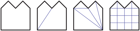
Figure 16.1 Various types of tessellation. The leftmost polygon is not tessellated, the next is partitioned into convex regions, the next is triangulated, and the rightmost is uniformly meshed.
Most tessellation algorithms work in two dimensions. They assume that all points in the polygon are in the same plane. However, some model creation systems can generate polygon facets that are badly warped and non-planar. A common case of this problem is the warped quadrilateral that is viewed nearly edge-on; this may form what is referred to as an hourglass or a bowtie quadrilateral. See Figure 16.2. While this particular polygon can be triangulated simply by creating a diagonal edge, more complex warped polygons cannot be so easily managed.

Figure 16.2 Warped quadrilateral viewed edge-on, forming an ill-defined bowtie or hourglass figure, along with the two possible triangulations.
When warped polygons are possible, one quick corrective action is to project the vertices onto a plane that is perpendicular to the polygon’s approximate normal. The normal for this plane is often found by computing the projected areas on the three orthogonal xy, xz, and yz planes. That is, the polygon’s area on the yz plane, found by dropping the x-coordinates, is the value for the x-component, on xz the y, and on xy the z. This method of computing an average normal is called Newell’s formula [1505, 1738].
The polygon cast onto this plane may still have self-intersection problems, where two or more of its edges cross. More elaborate and computationally expensive methods are then necessary. Zou et al. [1978] discuss previous work based on minimizing surface area or dihedral angles of the resulting tessellation, and present algorithms for optimizing a few non-planar polygons together in a set.
Schneider and Eberly [1574], Held [714], O’Rourke [1339], and de Berg et al. [135] each give an overview of a variety of triangulation methods. The most basic triangulation algorithm is to examine each line segment between any two given points on a polygon and see if it intersects or overlaps any edge of the polygon. If it does, the line segment cannot be used to split the polygon, so we examine the next possible pair of points. Else, split the polygon into two parts using this segment and triangulate these new polygons by the same method. This method is extremely slow, at O(n 3).
A more efficient method is ear clipping, which is O(n 2) when done as two processes. First, a pass is made over the polygon to find the ears, that is, to look at all triangles with vertex indices i, (i + 1), (i + 2) (modulo n) and check if the line segment i, (i + 2) does not intersect any polygon edges. If it does not, then triangle (i + 1) forms an ear. See Figure 16.3. Each ear available is removed from the polygon in turn, and the triangles at vertices i and (i + 2) are reexamined to see if they are now ears or not. Eventually all ears are removed and the polygon is triangulated. Other, more complex methods of triangulation are O(n log n) and some are effectively O(n) for typical cases. Pseudocode for ear clipping and other, faster triangulation methods is given by Schneider and Eberly [1574].
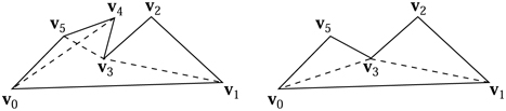
Figure 16.3 Ear clipping. A polygon with potential ears at v2, v4, and v5 shown. On the right, the ear at v4 is removed. The neighboring vertices v3 and v5 are reexamined to see if they now form ears; v5 does.
Rather than triangulating, partitioning a polygon into convex regions can be more efficient, both in storage and further computation costs. Code for a robust convexity test is given by Schorn and Fisher [1576]. Convex polygons can easily be represented by fans or strips of triangles, as discussed in Section 16.4. Some concave polygons can be treated as fans (such polygons are called star-shaped), but detecting these requires more work [1339, 1444]. Schneider and Eberly [1574] give two convex partitioning methods, a quick and dirty method and an optimal one.
Polygons are not always made of a single outline. Figure 16.4 shows a polygon made of three outlines, also called loops or contours. Such descriptions can always be converted to a single-outline polygon by carefully generating join edges (also called keyholed or bridge edges) between loops. Eberly [403] discusses how to find the mutually visible vertices that define such edges. This conversion process can also be reversed to retrieve the separate loops.

Figure 16.4 A polygon with three outlines converted to a single-outline polygon. Join edges are shown in red. Blue arrows inside the polygon show the order in which vertices are visited to make a single loop.
Writing a robust and general triangulator is a difficult undertaking. Various subtle bugs, pathological cases, and precision problems make foolproof code surprisingly tricky to create. One way to finesse the triangulation problem is to use the graphics accelerator itself to directly render a complex polygon. The polygon is rendered as a triangle fan to the stencil buffer. By doing so, the areas that should be filled are drawn an odd number of times, the concavities and holes drawn an even number. By using the invert mode for the stencil buffer, only the filled areas are marked at the end of this first pass. See Figure 16.5. In the second pass the triangle fan is rendered again, using the stencil buffer to allow only the filled area to be drawn. This method can even be used to render polygons with multiple outlines by drawing the triangles formed by every loop. The major drawbacks are that each polygon has to be rendered using two passes and the stencil buffer clears every frame, and that the depth buffer cannot be used directly. The technique can be useful for display of some user interactions, such as showing the interior of a complex selection area drawn on the fly.

Figure 16.5 Triangulation by rasterization, using odd/even parity for what area is visible. The polygon on the left is drawn into the stencil buffer as a fan of three triangles from vertex 0. The first triangle [0, 1, 2] (middle left) fills in its area, including space outside the polygon. Triangle [0, 2, 3] (middle right) fills its area, changing the parity of areas A and B to an even number of draws, thus making them empty. Triangle [0, 3, 4] (right) fills in the rest of the polygon.
16.2.1 Shading Problems
Sometimes data will arrive as quadrilateral meshes and must be converted into triangles for display. Once in a great while, a quadrilateral will be concave, in which case there is only one way to triangulate it. Otherwise, we may choose either of the two diagonals to split it. Spending a little time picking the better diagonal can sometimes give significantly better visual results.
There are a few different ways to decide how to split a quadrilateral. The key idea is to minimize differences at the vertices of the new edge. For a flat quadrilateral with no additional data at the vertices, it is often best to choose the shortest diagonal. For simple baked global illumination solutions that have a color per vertex, choose the diagonal which has the smaller difference between the colors [17]. See Figure 16.6. This idea of connecting the two least-different corners, as determined by some heuristic, is generally useful in minimizing artifacts.

Figure 16.6 The left figure is rendered as a quadrilateral; the middle is two triangles with upper right and lower left corners connected; the right shows what happens when the other diagonal is used. The middle figure is better visually than the right one.
Sometimes triangles cannot properly capture the intent of the designer. If a texture is applied to a warped quadrilateral, neither diagonal split preserves the intent. That said, simple horizontal interpolation over the non-triangulated quadrilateral, i.e., interpolating values from the left to the right edge, also fails. Figure 16.7 shows the problem. This problem arises because the image being applied to the surface is to be warped when displayed. A triangle has only three texture coordinates, so it can establish an affine transformation, but not a warp. At most, a basic (u, v) texture on a triangle can be sheared, not warped. Woo et al. [1901] discuss this problem further. Several solutions are possible:
- Warp the texture in advance and reapply this new image, with new texture coordinates.
- Tessellate the surface to a finer mesh. This only lessens the problem.
- Use projective texturing to warp the texture on the fly [691, 1470]. This has the undesirable effect of nonuniform spacing of the texture on the surface.
- Use a bilinear mapping scheme [691]. This is achievable with additional data per vertex.

Figure 16.7 The top left shows the intent of the designer, a distorted quadrilateral with a square texture map of an “R.” The two images on the right show the two triangulations and how they differ. The bottom row rotates all the polygons; the non-triangulated quadrilateral changes its appearance.
While texture distortion sounds like a pathological case, it happens to some extent any time the texture data applied does not match the proportions of the underlying quadrilateral, i.e., on almost any curved surface. One extreme case occurs with a common primitive: the cone. When a cone is textured and faceted, the triangle vertices at the tip of the cone have different normals. These vertex normals are not shared by the neighboring triangles, so shading discontinuities occur [647].
16.2.2 Edge Cracking and T-Vertices
Curved surfaces, discussed in detail in Chapter 17, are usually tessellated into meshes for rendering. This tessellation is done by stepping along the spline curves defining the surface and so computing vertex locations and normals. When we use a simple stepping method, problems can occur where spline surfaces meet. At the shared edge, the points for both surfaces need to coincide. Sometimes this may happen, due to the nature of the model, but often, without sufficient care, the points generated for one spline curve will not match those generated by its neighbor. This effect is called edge cracking, and it can lead to disturbing visual artifacts as the viewer peeks through the surface. Even if the viewer cannot see through the cracks, the seam is often visible because of differences in the way the shading is interpolated.
The process of fixing these cracks is called edge stitching. The goal is to make sure that all vertices along the (curved) shared edge are shared by both spline surfaces, so that no cracks appear. See Figure 16.8. Section 17.6.2 discusses using adaptive tessellation to avoid cracking for spline surfaces.

Figure 16.8 The left figure shows cracking where the two surfaces meet. The middle shows the cracking fixed by matching up edge points. The right shows the corrected mesh.
A related problem encountered when joining flat surfaces is that of T-vertices. This sort of problem can appear whenever two models’ edges meet, but do not share all vertices along them. Even though the edges should theoretically meet perfectly, if the renderer does not have enough precision in representing vertex locations on the screen, cracks can appear. Modern graphics hardware uses subpixel addressing [985] to help avoid this problem.
More obvious, and not due to precision, are the shading artifacts that can appear [114]. Figure 16.9 shows the problem, which can be fixed by finding such edges and making sure to share common vertices with bordering faces. An additional problem is the danger of creating degenerate (zero-area) triangles by using a simple fan algorithm. For example, in the figure, say the quadrilateral abcd in the upper right is triangulated into the triangles abc and acd. The triangle abc is a degenerate triangle, so point b is a T-vertex. Lengyel [1023] discusses how to find such vertices and provides code to properly retriangulate convex polygons. Cignoni et al. [267] describe a method to avoid creating degenerate (zero-area) triangles when the T-vertices’ locations are known. Their algorithm is O(n) and is guaranteed to produce at most one triangle strip and fan.

Figure 16.9 In the top row, the underlying mesh of a surface shows a shading discontinuity. Vertex b is a T-vertex, as it belongs to the triangles to the left of it, but is not a part of the triangle acd. One solution is to add this T-vertex to this triangle and create triangles abd and bcd (not shown). Long and thin triangles are more likely to cause other shading problems, so retriangulating is often a better solution, shown in the bottom row.
16.3 Consolidation
Once a model has passed through any tessellation algorithms needed, we are left with a set of polygons representing the model. There are a few operations that may be useful for displaying these data. The simplest is checking whether the polygon itself is properly formed, that it has at least three unique vertex locations, and that they are not collinear. For example, if two vertices in a triangle match, then it has no area and can be discarded. Note that in this section we are truly referring to polygons, not just triangles. Depending on your goals, it can be more efficient to store each polygon, instead of immediately converting it to triangles for display. Triangulating creates more edges, which in turn creates more work for the operations that follow.
One procedure commonly applied to polygons is merging, which finds shared vertices among faces. Another operation is called orientation, where all polygons forming a surface are made to face the same direction. Orienting a mesh is important for several different algorithms, such as backface culling, crease edge detection, and correct collision detection and response. Related to orientation is vertex normal generation, where surfaces are made to look smooth. We call all these types of techniques consolidation algorithms.
16.3.1 Merging
Some data comes in the form of disconnected polygons, often termed a polygon soup or triangle soup. Storing separate polygons wastes memory, and displaying separate polygons is extremely inefficient. For these reasons and others, individual polygons are usually merged into a polygon mesh. At its simplest, a mesh consists of a list of vertices and a set of outlines. Each vertex contains a position and other optional data, such as the shading normal, texture coordinates, tangent vectors, and color. Each polygon outline has a list of integer indices. Each index is a number from 0 to n - 1, where n is the number of vertices and so points to a vertex in the list. In this way, each vertex can be stored just once and shared by any number of polygons. A triangle mesh is a polygon mesh that contains only triangles. Section 16.4.5 discusses mesh storage schemes in depth.
Given a set of disconnected polygons, merging can be done in several ways. One method is to use hashing [542, 1135]. Initialize a vertex counter to zero. For each polygon, attempt to add each of its vertices in turn to a hash table, hashing based on the vertex values. If a vertex is not already in the table, store it there, along with the vertex counter value, which is then incremented; also store the vertex in the final vertex list. If instead the vertex is found to match, retrieve its stored index. Save the polygon with the indices that point to the vertices. Once all polygons are processed, the vertex and index lists are complete.
Model data sometimes comes in with separate polygons’ vertices being extremely close, but not identical. The process of merging such vertices is called welding. Efficiently welding vertices can be done by using sorting along with a looser equality function for the position [1135].
16.3.2 Orientation
One quality-related problem with model data is face orientation. Some model data come in oriented properly, with surface normals either explicitly or implicitly pointing in the correct directions. For example, in CAD work, the standard is that the vertices in the polygon outline proceed in a counterclockwise direction when the frontface is viewed. This is called the winding direction and the triangles use the right-hand rule. Think of the fingers of your right hand wrapping around the polygon’s vertices in counterclockwise order. Your thumb then points in the direction of the polygon’s normal. This orientation is independent of the left-handed or right-handed view-space or world-coordinate orientation used, as it relies purely on the ordering of the vertices in the world, when looking at the front of the triangle. That said, if a reflection matrix is applied to an oriented mesh, each triangle’s normal will be reversed compared to its winding direction.
Given a reasonable model, here is one approach to orient a polygonal mesh:
- Form edge-face structures for all polygons.
- Sort or hash the edges to find which edges match.
- Find groups of polygons that touch each other.
- For each group, flip faces as needed to obtain consistency.
The first step is to create a set of half-edge objects. A half-edge is an edge of a polygon, with a pointer to its associated face (polygon). Since an edge is normally shared by two polygons, this data structure is called a half-edge. Create each halfedge with its first vertex stored before the second vertex, using sorting order. One vertex comes before another in sorting order if its x-coordinate value is smaller. If the x-coordinates are equal, then the y-value is used; if these match, then z is used. For example, vertex (−3, 5, 2) comes before vertex (−3, 6, −8); the −3s match, but 5 < 6.
The goal is to find which edges are identical. Since each edge is stored so that the first vertex is less than the second, comparing edges is a matter of comparing first to first and second to second vertices. No permutations such as comparing one edge’s first vertex to another’s second vertex are needed. A hash table can be used to find matching edges [19, 542]. If all vertices have previously been merged, so that half-edges use the same vertex indices, then each half-edge can be matched by putting it on a temporary list associated with its first vertex index. A vertex has an average of 6 edges attached to it, making edge matching extremely rapid once grouped [1487]. Once the edges are matched, connections among neighboring polygons are known, forming an adjacency graph. For a triangle mesh, this can be represented as a list for each triangle of its (up to) three neighboring triangle faces. Any edge that does not have two neighboring polygons is a boundary edge. The set of polygons that are connected by edges forms a continuous group. For example, a teapot model has two groups, the pot and the lid.
The next step is to give the mesh orientation consistency, e.g., we usually want all polygons to have counterclockwise outlines. For each continuous group of polygons, choose an arbitrary starting polygon. Check each of its neighboring polygons and determine whether the orientation is consistent. If the direction of traversal for the edge is the same for both polygons, then the neighboring polygon must be flipped. See Figure 16.10. Recursively check the neighbors of these neighbors, until all polygons in a continuous group are tested once.

Figure 16.10 A starting polygon S is chosen and its neighbors are checked. Because the vertices in the edge shared by S and B are traversed in the same order (from x to y), the outline for B needs to be reversed to make it follow the right-hand rule.
Although all the faces are properly oriented at this point, they could all be oriented inward. In most cases we want them facing outward. One quick test for whether all faces should be flipped is to compute the signed volume of the group and check the sign. If it is negative, reverse all the loops and normals. Compute this volume by calculating the signed volume scalar triple product for each triangle and summing these. Look for the volume calculation in our online linear algebra appendix at realtimerendering.com. This method works well for solid objects but is not foolproof. For example, if the object is a box forming a room, the user wants its normals to face inward toward the camera. If the object is not a solid, but rather a surface description, the problem of orienting each surface can become tricky to perform automatically. If, say, two cubes touch along an edge and are a part of the same mesh, that edge would be shared by four polygons, making orientation more difficult. One-sided objects such as M¨obius strips can never be fully oriented, since there is no separation of inside and outside. Even for well-behaved surface meshes it can be difficult to determine which side should face outward. Takayama et al. [1736] discuss previous work and present their own solution, casting random rays from each facet and determining which orientation is more visible from the outside.
16.3.3 Solidity
Informally, a mesh forms a solid if it is oriented and all the polygons visible from the outside have the same orientation. In other words, only one side of the mesh is visible. Such polygonal meshes are called closed or watertight.
Knowing an object is solid means backface culling can be used to improve display efficiency, as discussed in Section 19.2. Solidity is also a critical property for objects casting shadow volumes (Section 7.3) and for several other algorithms. For example, a 3D printer requires that the mesh it prints be solid.
The simplest test for solidity is to check if every polygon edge in the mesh is shared by exactly two polygons. This test is sufficient for most data sets. Such a surface is loosely referred to as being manifold, specifically, two-manifold. Technically, a manifold surface is one without any topological inconsistencies, such as having three or more polygons sharing an edge or two or more corners touching each other. A continuous surface forming a solid is a manifold without boundaries.
16.3.4 Normal Smoothing and Crease Edges
Some polygon meshes form curved surfaces, but the polygon vertices do not have normal vectors, so they cannot be rendered with the illusion of curvature. See Figure 16.11.

Figure 16.11 The object on the left does not have normals per vertex; the one on the right does.
Many model formats do not provide surface edge information. See Section 15.2 for the various types of edges. These edges are important for several reasons. They can highlight an area of the model made of a set of polygons or can help in nonphotorealistic rendering. Because they provide important visual cues, such edges are often favored to avoid being simplified by progressive mesh algorithms (Section 16.5).
Reasonable crease edges and vertex normals can usually be derived with some success from an oriented mesh. Once the orientation is consistent and the adjacency graph is derived, vertex normals can be generated by smoothing techniques. The model’s format may provide help by specifying smoothing groups for the polygon mesh. Smoothing group values are used to explicitly define which polygons in a group belong together to make up a curved surface. Edges between different smoothing groups are considered sharp.
Another way to smooth a polygon mesh is to specify a crease angle. This value is compared to the dihedral angle, which is the angle between the plane normals of two polygons. Values typically range from 20 to 50 degrees. If the dihedral angle between two neighboring polygons is found to be lower than the specified crease angle, then these two polygons are considered to be in the same smoothing group. This technique is sometimes called edge preservation.
Using a crease angle can sometimes give an improper amount of smoothing, rounding edges that should be creased, or vice versa. Often experimentation is needed, and no single angle may work perfectly for a mesh. Even smoothing groups have limitations. One example is when you pinch a sheet of paper in the middle. The sheet could be thought of as a single smoothing group, yet it has creases within it, which a smoothing group would smooth away. The modeler then needs multiple overlapping smoothing groups, or direct crease edge definition on the mesh. Another example is a cone made from triangles. Smoothing the cone’s whole surface gives the peculiar result that the tip has one normal pointing directly out along the cone’s axis. The cone tip is a singularity. For perfect representation of the interpolated normal, each triangle would need to be more like a quadrilateral, with two normals at this tip location [647]. Fortunately, such problematic cases are usually rare. Once a smoothing group is found, vertex normals can be computed for vertices shared within the group. The standard textbook solution for finding the vertex normal is to average the surface normals of the polygons sharing the vertex [541, 542]. However, this method can lead to inconsistent and poorly weighted results. Thu¨rmer and Wu¨thrich [1770] present an alternate method, in which each polygon normal’s contribution is weighted by the angle it forms at the vertex. This method has the desirable property of giving the same result whether a polygon sharing a vertex is triangulated or not. If the tessellated polygon turned into, say, two triangles sharing the vertex, the average normal method would incorrectly exert twice the influence from the two triangles as it would for the original polygon. See Figure 16.12.

Figure 16.12 On the left, the surface normals of a quadrilateral and two triangles are averaged to give a vertex normal. In the middle, the quadrilateral has been triangulated. This results in the average normal shifting, since each polygon’s normal is weighted equally. On the right, Thu¨rmer and Wu¨thrich’s method weights each normal’s contribution by its angle between the pair of edges forming it, so triangulation does not shift the normal.
Max [1146] gives a different weighting method, based on the assumption that long edges form polygons that should affect the normal less. This type of smoothing may be superior when using simplification techniques, as larger polygons that are formed will be less likely to follow the surface’s curvature.
Jin et al. [837] provide a comprehensive survey of these and other methods, concluding that weighting by angle is either the best or among the best under various conditions. Cignoni [268] implements a few methods in Meshlab and notes about the same. He also warns against weighting the contribution of each normal by the area of its associated triangle.
For heightfields, Shankel [1614] shows how taking the difference in heights of the neighbors along each axis can be used to rapidly approximate smoothing using the angle-weighted method. For a given point p and four neighboring points, p x−1 and p x+1 on the x-axis of the heightfield and p y−1 and p y+1 on the y-axis, a close approximation of the (unnormalized) normal at p is
16.4 Triangle Fans, Strips, and Meshes
A triangle list is the simplest, and usually least efficient, way to store and display a set of triangles. The vertex data for each triangle is put in a list, one after another. Each triangle has its own separate set of three vertices, so there is no sharing of vertex data among triangles. A standard way to increase graphics performance is to send groups of triangles that share vertices through the graphics pipeline. Sharing means fewer calls to the vertex shader, so less points and normals need to be transformed. Here we describe a variety of data structures that share vertex information, starting with triangle fans and strips and progressing to more elaborate, and more efficient, forms for rendering surfaces.
16.4.1 Fans
Figure 16.13 shows a triangle fan. This data structure shows how we can form triangles and have the storage cost be less than three vertices per triangle. The vertex shared by all triangles is called the center vertex and is vertex 0 in the figure. For the starting triangle 0, send vertices 0, 1, and 2 (in that order). For subsequent triangles, the center vertex is always used together with the previously sent vertex and the vertex currently being sent. Triangle 1 is formed by sending vertex 3, thereby creating a triangle defined by vertices 0 (always included), 2 (the previously sent vertex), and 3. Triangle 2 is constructed by sending vertex 4, and so on. Note that a general convex polygon is trivial to represent as a triangle fan, since any of its points can be used as the starting, center vertex.

Figure 16.13 The left figure illustrates the concept of a triangle fan. Triangle T 0 sends vertices v0 (the center vertex), v1, and v2. The subsequent triangles, T i (i > 0), send only vertex vi+2. The right figure shows a convex polygon, which can always be turned into one triangle fan.
A triangle fan of n vertices is defined as an ordered vertex list
(16.2)
where v0 is the center vertex, with a structure imposed upon the list indicating that triangle i is
where 0 ≤ i < n − 2.
(16.3)
If a triangle fan consists of m triangles, then three vertices are sent for the first, followed by one more for each of the remaining m − 1 triangles. This means that the average number of vertices, v a , sent for a sequential triangle fan of length m, can be expressed as
(16.4)
As can easily be seen, v a → 1 as m → ∞. This might not seem to have much relevance for real-world cases, but consider a more reasonable value. If m = 5, then v a = 1.4, which means that, on average, only 1.4 vertices are sent per triangle.
16.4.2 Strips
Triangle strips are like triangle fans, in that vertices in previous triangles are reused. Instead of a single center point and the previous vertex getting reused, it is two vertices of the previous triangle that help form the next triangle. Consider Figure 16.14. If these triangles are treated as a strip, then a more compact way of sending them to the rendering pipeline is possible. For the first triangle (denoted T 0), all three vertices (denoted v0, v1, and v2) are sent, in that order. For subsequent triangles in this strip, only one vertex has to be sent, since the other two have already been sent with the previous triangle. For example, sending triangle T 1, only vertex v3 is sent, and the vertices v1 and v2 from triangle T 0 are used to form triangle T 1. For triangle T 2, only vertex v4 is sent, and so on through the rest of the strip.

Figure 16.14 A sequence of triangles that can be represented as one triangle strip. Note that the orientation changes from triangle to triangle in the strip, and that the first triangle in the strip sets the orientation of all triangles. Internally, counterclockwise order is kept consistent by traversing vertices [0, 1, 2], [1, 3, 2], [2, 3, 4], [3, 5, 4], and so on.
A sequential triangle strip of n vertices is defined as an ordered vertex list,
(16.5)
with a structure imposed upon it indicating that triangle i is
(16.6)
where 0 ≤ i < n − 2. This sort of strip is called sequential because the vertices are sent in the given sequence. The definition implies that a sequential triangle strip of n vertices has n − 2 triangles.
The analysis of the average number of vertices for a triangle strip of length m (i.e., consisting of m triangles), also denoted v a , is the same as for triangle fans (see Equation 16.4), since they have the same start-up phase and then send only one vertex per new triangle. Similarly, when m → ∞, v a for triangle strips naturally also tends toward one vertex per triangle. For m = 20, v a = 1.1, which is much better than 3 and is close to the limit of 1.0. As with triangle fans, the start-up cost for the first triangle, always costing three vertices, is amortized over the subsequent triangles.
The attractiveness of triangle strips stems from this fact. Depending on where the bottleneck is located in the rendering pipeline, there is a potential for saving up to two thirds of the time spent rendering with simple triangle lists. The speedup is due to avoiding redundant operations such as sending each vertex twice to the graphics hardware, then performing matrix transformations, clipping, and other operations on each. Triangle strips are useful for objects such as blades of grass or other objects where edge vertices are not reused by other strips. Because of its simplicity, strips are used by the geometry shader when multiple triangles are output.
There are several variants on triangles strips, such as not imposing a strict sequence on the triangles, or using doubled vertices or a restart index value so that multiple disconnected strips can be stored in a single buffer. There once was considerable research on how best to decompose an arbitrary mesh of triangles into strips [1076]. Such efforts have died off, as the introduction of indexed triangle meshes allowed better vertex data reuse, leading to both faster display and usually less overall memory needed.
16.4.3 Triangle Meshes
Triangle fans and strips still have their uses, but the norm on all modern GPUs is to use triangle meshes with a single index list (Section 16.3.1) for complex models [1135]. Strips and fans allow some data sharing, but mesh storage allows even more. In a mesh an additional index array keeps track of which vertices form the triangles. In this way, a single vertex can be associated with several triangles.
The Euler-Poincar′e formula for connected planar graphs [135] helps in determining the average number of vertices that form a closed mesh:
(16.7)
Here v is the number of vertices, e is the number of edges, f is the number of faces, and g is the genus. The genus is the number of holes in the object. As an example, a sphere has genus 0 and a torus has genus 1. Each face is assumed to have one loop.
If faces can have multiple loops, the formula becomes
(16.8)
where l is the number of loops.
For a closed (solid) model, every edge has two faces, and every face has at least three edges, so 2e ≥ 3f . If the mesh is all triangles, as the GPU demands, then 2e = 3f . Assuming a genus of 0 and substituting 1.5f for e in the formula yields f ≤ 2v − 4. If all faces are triangles, then f = 2v − 4.
For large closed triangle meshes, the rule of thumb then is that the number of triangles is about equal to twice the number of vertices. Similarly, we find that each vertex is connected to an average of nearly six triangles (and, therefore, six edges). The number of edges connected to a vertex is called its valence. Note that the network of the mesh does not affect the result, only the number of triangles does. Since the average number of vertices per triangle in a strip approaches one, and the number of vertices is twice that of triangles, every vertex has to be sent twice (on average) if a large mesh is represented by triangle strips. At the limit, triangle meshes can send 0.5 vertices per triangle.
Note that this analysis holds for only smooth, closed meshes. As soon as there are boundary edges (edges not shared between two polygons), the ratio of vertices to triangles increases. The Euler-Poincar′e formula still holds, but the outer boundary of the mesh has to be considered a separate (unused) face bordering all exterior edges. Similarly, each smoothing group in any model is effectively its own mesh, since GPUs need to have separate vertex records with differing normals along sharp edges where two groups meet. For example, the corner of a cube will have three normals at a single location, so three vertex records are stored. Changes in textures or other vertex data can also cause the number of distinct vertex records to increase.
Theory predicts we need to process about 0.5 vertices per triangle. In practice, vertices are transformed by the GPU and put in a first-in, first-out (FIFO) cache, or in something approximating a least recently used (LRU) system [858]. This cache holds post-transform results for each vertex run through the vertex shader. If an incoming vertex is located in this cache, then the cached post-transform results can be used without calling the vertex shader, providing a significant performance increase. If instead the triangles in a triangle mesh are sent down in random order, the cache is unlikely to be useful. Triangle strip algorithms optimize for a cache size of two, i.e., the last two vertices used. Deering and Nelson [340] first explored the idea of storing vertex data in a larger FIFO cache by using an algorithm to determine in which order to add the vertices to the cache.
FIFO caches are limited in size. For example, the PLAYSTATION 3 system holds about 24 vertices, depending on the number of bytes per vertex. Newer GPUs have not increased this cache significantly, with 32 vertices being a typical maximum.
Hoppe [771] introduces an important measurement of cache reuse, the average cache miss ratio (ACMR). This is the average number of vertices that need to be processed per triangle. It can range from 3 (every vertex for every triangle has to be reprocessed each time) to 0.5 (perfect reuse on a large closed mesh; no vertex is reprocessed). If the cache size is as large as the mesh itself, the ACMR is identical to the theoretical vertex to triangle ratio. For a given cache size and mesh ordering, the ACMR can be computed precisely, so describing the efficiency of any given approach for that cache size.
16.4.4 Cache-Oblivious Mesh Layouts
The ideal order for triangles in an mesh is one in which we maximize the use of the vertex cache. Hoppe [771] presents an algorithm that minimizes the ACMR for a mesh, but the cache size has to be known in advance. If the assumed cache size is larger than the actual cache size, the resulting mesh can have significantly less benefit. Solving for different-sized caches may yield different optimal orderings. For when the target cache size is unknown, cache-oblivious mesh layout algorithms have been developed that yield orderings that work well, regardless of size. Such an ordering is sometimes called a universal index sequence.
Forsyth [485] and Lin and Yu [1047] provide rapid greedy algorithms that use similar principles. Vertices are given scores based on their positions in the cache and by the number of unprocessed triangles attached to them. The triangle with the highest combined vertex score is processed next. By scoring the three most recently used vertices a little lower, the algorithm avoids simply making triangle strips and instead creates patterns similar to a Hilbert curve. By giving higher scores to vertices with fewer triangles still attached, the algorithm tends to avoid leaving isolated triangles behind. The average cache miss ratios achieved are comparable to those of more costly and complex algorithms. Lin and Yu’s method is a little more complex but uses related ideas. For a cache size of 12, the average ACMR for a set of 30 unoptimized models was 1.522; after optimization, the average dropped to 0.664 or lower, depending on cache size.
Sander et al. [1544] give an overview of previous work and present their own faster (though not cache-size oblivious) method, called Tipsify. One addition is that they also strive to put the outermost triangles early on in the list, to minimize overdraw (Section 18.4.5). For example, imagine a coffee cup. By rendering the triangles forming the outside of the cup first, the later triangles inside are likely to be hidden from view. Storsj¨o [1708] contrasts and compares Forsyth’s and Sander’s methods, and provides implementations of both. He concludes that these methods provide layouts that are near the theoretical limits. A newer study by Kapoulkine [858] compares four cache-aware vertex-ordering algorithms on three hardware vendors’ GPUs. Among his conclusions are that Intel uses a 128-entry FIFO, with each vertex using three or more entries, and that AMD’s and NVIDIA’s systems approximate a 16-entry LRU cache. This architectural difference significantly affects algorithm behavior. He finds that Tipsify [1544] and, to a lesser extent, Forsyth’s algorithm [485] perform relatively well across these platforms.
To conclude, offline preprocessing of triangle meshes can noticeably improve vertex cache performance, and the overall frame rate when this vertex stage is the bottleneck. It is fast, effectively O(n) in practice. There are several open-source versions available [485]. Given that such algorithms can be applied automatically to a mesh and that such optimization has no additional storage cost and does not affect other tools in the toolchain, these methods are often a part of a mature development system. Forsyth’s algorithm appears to be part of the PLAYSTATION mesh processing toolchain, for example. While the vertex post-transform cache has evolved due to modern GPUs’ adoption of a unified shader architecture, avoiding cache misses is still an important concern [530].
16.4.5 Vertex and Index Buffers/Arrays
One way to provide a modern graphics accelerator with model data is by using what DirectX calls vertex buffers and OpenGL calls vertex buffer objects (VBOs). We will go with the DirectX terminology in this section. The concepts presented have OpenGL equivalents.
The idea of a vertex buffer is to store model data in a contiguous chunk of memory. A vertex buffer is an array of vertex data in a particular format. The format specifies whether a vertex contains a normal, texture coordinates, a color, or other specific information. Each vertex has its data in a group, one vertex after another. The size in bytes of a vertex is called its stride. This type of storage is called an interleaved buffer. Alternately, a set of vertex streams can be used. For example, one stream could hold an array of positions {p0p1p2 . . .} and another a separate array of normals {n0n1n2 . . .}.
In practice, a single buffer containing all data for each vertex is generally more efficient on GPUs, but not so much that multiple streams should be avoided [66, 1494]. The main cost of multiple streams is additional API calls, possibly worth avoiding if the application is CPU-bound but otherwise not significant [443].
Wihlidal [1884] discusses different ways multiple streams can help rendering system performance, including API, caching, and CPU processing advantages. For example, SSE and AVX for vector processing on the CPU are easier to apply to a separate stream. Another reason to use multiple streams is for more efficient mesh updating. If, say, just the vertex location stream is changing over time, it is less costly to update this one attribute buffer than to form and send an entire interleaved stream [1609].
How the vertex buffer is accessed is up to the device’s DrawPrimitive method.
The data can be treated as:
- A list of individual points.
- A list of unconnected line segments, i.e., pairs of vertices.
- A single polyline.
- A triangle list, where each group of three vertices forms a triangle, e.g., vertices [0, 1, 2] form one, [3, 4, 5] form the next, and so on.
- A triangle fan, where the first vertex forms a triangle with each successive pair of vertices, e.g., [0, 1, 2], [0, 2, 3], [0, 3, 4].
- A triangle strip, where every group of three contiguous vertices forms a triangle, e.g., [0, 1, 2], [1, 2, 3], [2, 3, 4].
In DirectX 10 on, triangles and triangle strips can also include adjacent triangle vertices, for use by the geometry shader (Section 3.7).
The vertex buffer can be used as is or referenced by an index buffer. The indices in an index buffer hold the locations of vertices in a vertex buffer. Indices are stored as 16-bit unsigned integers, or 32-bit if the mesh is large and the GPU and API support it (Section 16.6). The combination of an index buffer and vertex buffer is used to display the same types of draw primitives as a “raw” vertex buffer. The difference is that each vertex in the index/vertex buffer combination needs to be stored only once in its vertex buffer, versus repetition that can occur in a vertex buffer without indexing.
The triangle mesh structure is represented by an index buffer. The first three indices stored in the index buffer specify the first triangle, the next three the second, and so on. This arrangement is called an indexed triangle list, where the indices themselves form a list of triangles. OpenGL binds the index buffer and vertex buffer(s) together with vertex format information in a vertex array object (VAO). Indices can also be arranged in triangle strip order, which saves on index buffer space. This format, the indexed triangle strip, is rarely used in practice, in that creating such sets of strips for a large mesh takes some effort, and all tools that process geometry also then need to support this format. See Figure 16.15 for examples of vertex and index buffer structures.
Which structure to use is dictated by the primitives and the program. Displaying a simple rectangle is easily done with just a vertex buffer using four vertices as a two- triangle tristrip or fan. One advantage of the index buffer is data sharing, as discussed earlier. Another advantage is simplicity, in that triangles can be in any order and configuration, not having the lock-step requirements of triangle strips. Lastly, the amount of data that needs to be transferred and stored on the GPU is usually smaller when an index buffer is used. The small overhead of including an indexed array is far outweighed by the memory savings achieved by sharing vertices.
An index buffer and one or more vertex buffers provide a way of describing a polygonal mesh. However, the data are typically stored with the goal of GPU rendering efficiency, not necessarily the most compact storage. For example, one way to store a cube is to save its eight corner locations in one array, and its six different normals in another, along with the six four-index loops that define its faces. Each vertex location is then described by two indices, one for the vertex list and one for the normal list. Texture coordinates are represented by yet another array and a third index. This compact representation is used in many model file formats, such as Wavefront OBJ. On the GPU, only one index buffer is available. A single vertex buffer would store 24 different vertices, as each corner location has three separate normals, one for each neighboring face. The index buffer would store indices defining the 12 triangles forming the surface. Masserann [1135] discusses efficiently turning such file descriptions into compact and efficient index/vertex buffers, versus lists of unindexed triangles that do not share vertices. More compact schemes are possible by such methods as storing the mesh in texture maps or buffer textures and using the vertex shader’s texture fetch or pulling mechanisms, but they come at the performance penalty of not being able to use the post-transform vertex cache [223, 1457].
For maximum efficiency, the order of the vertices in the vertex buffer should match the order in which they are accessed by the index buffer. That is, the first three vertices referenced by the first triangle in the index buffer should be first three in the vertex buffer. When a new vertex is encountered in the index buffer, it should then be next in the vertex buffer. Giving this order minimizes cache misses in the pre-transform vertex cache, which is separate from the post-transform cache discussed in Section 16.4.4. Reordering the data in the vertex buffer is a simple operation, but can be as important to performance as finding an efficient triangle order for the post-transform vertex cache [485].

Figure 16.15 Different ways of defining primitives, in rough order of most to least memory use from top to bottom: separate triangles, as a vertex triangle list, as triangle strips of two or one data streams, and as an index buffer listing separate triangles or in triangle strip order.

Figure 16.16 In the upper left is a heightfield of Crater Lake rendered with 200,000 triangles. The upper right figure shows this model simplified down to 1000 triangles in a triangulated irregular network (TIN). The underlying simplified mesh is shown at the bottom. (Images courtesy of Michael Garland.)
There are higher-level methods for allocating and using vertex and index buffers to achieve greater efficiency. For example, a buffer that does not change can be stored on the GPU for use each frame, and multiple instances and variations of an object can be generated from the same buffer. Section 18.4.2 discusses such techniques in depth.
The ability to send processed vertices to a new buffer using the pipeline’s stream output functionality (Section 3.7.1) allows a way to process vertex buffers on the GPU without rendering them. For example, a vertex buffer describing a triangle mesh could be treated as a simple set of points in an initial pass. The vertex shader could be used to perform per-vertex computations as desired, with the results sent to a new vertex buffer using stream output. On a subsequent pass, this new vertex buffer could be paired with the original index buffer describing the mesh’s connectivity, to further process and display the resulting mesh.
16.5 Simplification
Mesh simplification, also known as data reduction or decimation, is the process of taking a detailed model and reducing its triangle count while attempting to preserve its appearance. For real-time work this process is done to reduce the number of vertices stored and sent down the pipeline. This can be important in making the application scalable, as less powerful machines may need to display lower numbers of triangles. Model data may also be received with more tessellation than is necessary for a reasonable representation. Figure 16.16 gives a sense of how the number of stored triangles can be reduced by data reduction techniques.
Luebke [1091, 1092] identifies three types of mesh simplification: static, dynamic, and view-dependent. Static simplification is the idea of creating separate level of detail (LOD) models before rendering begins, and the renderer chooses among these. This form is covered in Section 19.9. Offline simplification can also be useful for other tasks, such as providing coarse meshes for subdivision surfaces to refine [1006, 1007]. Dynamic simplification gives a continuous spectrum of LOD models instead of a few discrete models, and so such methods are referred to as continuous level of detail (CLOD) algorithms. View-dependent techniques are meant for where the level of detail varies within the model. Specifically, terrain rendering is a case in which the nearby areas in view need detailed representation while those in the distance are at a lower level of detail. These two types of simplification are discussed in this section.
16.5.1 Dynamic Simplification
One method of reducing the triangle count is to use an edge collapse operation, where an edge is removed by moving its two vertices to coincide. See Figure 16.17 for an example of this operation in action. For a solid model, an edge collapse removes a total of two triangles, three edges, and one vertex. So, a closed model with 3000 triangles would have 1500 edge collapses applied to it to reduce it to zero faces. The rule of thumb is that a closed triangle mesh with v vertices has about 2v faces and 3v edges. This rule can be derived using the Euler-Poincar′e formula that f − e + v = 2 for a solid’s surface (Section 16.4.3).

Figure 16.17 On the left is the figure before the uv edge collapse occurs; the right figure shows point u collapsed into point v, thereby removing triangles A and B and edge uv.
The edge collapse process is reversible. By storing the edge collapses in order, we can start with the simplified model and reconstruct the complex model from it. This characteristic can be useful for network transmission of models, in that the edge- collapsed version of the database can be sent in an efficiently compressed form and progressively built up and displayed as the model is received [768, 1751]. Because of this feature, this simplification process is often referred to as view-independent progressive meshing (VIPM).
In Figure 16.17, u was collapsed into the location of v, but v could have been collapsed into u. A simplification system limited to just these two possibilities is using a subset placement strategy. An advantage of this strategy is that, if we limit the possibilities, we may implicitly encode the choice made [516, 768]. This strategy is faster because fewer possibilities need to be evaluated, but it also can yield lower- quality approximations because a smaller solution space is examined.
When using an optimal placement strategy, we examine a wider range of possibilities. Instead of collapsing one vertex into another, both vertices for an edge are contracted to a new location. Hoppe [768] examines the case in which u and v both move to some location on the edge joining them. He notes that to improve compression of the final data representation, the search can be limited to checking the midpoint. Garland and Heckbert [516] go further, solving a quadratic equation to find an optimal position, one that may be located off of the edge. The advantage of optimal placement strategies is that they tend to give higher-quality meshes. The disadvantages are extra processing, code, and memory for recording this wider range of possible placements.
To determine the best point placement, we perform an analysis on the local neighborhood. This locality is an important and useful feature for several reasons. If the cost of an edge collapse depends on just a few local variables (e.g., edge length and face normals near the edge), the cost function is easy to compute, and each collapse affects only a few of its neighbors. For example, say a model has 3000 possible edge collapses that are computed at the start. The edge collapse with the lowest cost-function value is performed. Because it influences only a few nearby triangles and their edges, only those edge collapse possibilities whose cost functions are affected by these changes need to be recomputed (say, 10 instead of 3000), and the list requires only a minor bit of resorting. Because an edge-collapse affects only a few other edge-collapse cost values, a good choice for maintaining this list of cost values is a heap or other priority queue [1649].
Some contractions must be avoided regardless of cost. See an example in Figure 16.18. These can be detected by checking whether a neighboring triangle flips its normal direction due to a collapse.

Figure 16.18 Example of a bad collapse. On the left is a mesh before collapsing vertex u into v. On the right is the mesh after the collapse, showing how edges now cross.
The collapse operation itself is an edit of the model’s database. Data structures for storing these collapses are well documented [481, 770, 1196, 1726]. Each edge collapse is analyzed with a cost function, and the one with the smallest cost value is performed next. The best cost function can and will vary with the type of model and other factors [1092]. Depending on the problem being solved, the cost function may make trade-offs among speed, quality, robustness, and simplicity. It may also be tailored to maintain surface boundaries, material locations, lighting effect, symmetry along an axis, texture placement, volume, or other constraints.
We will present Garland and Heckbert’s quadric error metric (QEM) cost function [515, 516] in order to give a sense of how such functions work. This function is of general use in a large number of situations. In contrast, in earlier research Garland and Heckbert [514] found using the Hausdorff distance best for terrain simplification, and others have borne this out [1496]. This function is simply the longest distance a vertex in the simplified mesh is from the original mesh. Figure 16.16 shows a result from using this metric.
For a given vertex there is a set of triangles that share it, and each triangle has a plane equation associated with it. The QEM cost function for moving a vertex is the sum of the squared distances between each of these planes and the new location. More formally,
is the cost function for new location v and m planes, where n i is the plane i’s normal and d i its offset from the origin.
An example of two possible contractions for the same edge is shown in Figure 16.19. Say the cube is two units wide. The cost function for collapsing e into c (e → c) will be 0, because the point e does not move off of the planes it shares when it goes to c. The cost function for c → e will be 1, because c moves away from the plane of the right face of the cube by a squared distance of 1. Because it has a lower cost, the e → c collapse would be preferred over c → e.

Figure 16.19 The left figure shows a cube with an extra point along one edge. The middle figure shows what happens if this point e is collapsed to corner c. The right figure shows c collapsed to e.
This cost function can be modified in various ways. Imagine two triangles that share an edge that form a sharp edge, e.g., they are part of a fish’s fin or turbine blade. The cost function for collapsing a vertex on this edge is low, because a point sliding along one triangle does not move far from the other triangle’s plane. The basic function’s cost value is related to the volume change of removing the feature, but is not a good indicator of its visual importance. One way to maintain an edge with a sharp crease is to add an extra plane that includes the edge and has a normal that is the average of the two triangle normals. Now vertices that move far from this edge will have a higher cost function [517]. A variation is to weight the cost function by the change in the areas of the triangles.
Another type of extension is to use a cost function based on maintaining other surface features. For example, the crease and boundary edges of a model are important in portraying it, so these should be made less likely to be modified. See Figure 16.20. Other surface features worth preserving are locations where there are material changes, texture map edges, and color-per-vertex changes [772]. See Figure 16.21.

Figure 16.20 Mesh simplification. Upper left shows the original mesh of 13,546 faces, upper right is simplified to 1,000 faces, lower left to 500 faces, lower right to 150 faces [770]. (Images c 1996 Microsoft. All rights reserved.)

Figure 16.21 Mesh simplification. Top row: with mesh and simple gray material. Bottom row: with textures. From left to right: the models contain 51,123, 6,389, and 1,596 triangles. The texture on the model is maintained as possible, though some distortion creeps in as the triangle count falls. (Images c 2016 Microsoft. All rights reserved.)
One serious problem that occurs with most simplification algorithms is that textures often deviate in a noticeable way from their original appearance [1092]. As edges are collapsed, the underlying mapping of the texture to the surface can become distorted. Also, texture coordinate values can match at boundaries but belong to different regions where the texture is applied, e.g., along a central edge where a model is mirrored. Caillaud et al. [220] survey a variety of previous approaches and present their own algorithm that handles texture seams.
Speed can be another concern. In systems where users create their own content, such as in a CAD system, level of detail models need to be created on the fly. Performing simplification using the GPU has met with some success [1008]. Another approach is to use a simpler simplification algorithm, such as vertex clustering [1088, 1511]. The core idea of this approach is to overlay the model with a three-dimensional voxel grid or similar structure. Any vertices in a voxel are moved to a “best” vertex location for that cell. Doing so may eliminate some triangles, when two or more of each triangle’s vertices land in the same location, making it degenerate. This algorithm is robust, the connectivity of the mesh is not needed, and separate meshes can easily be aggregated into one. However, the basic vertex clustering algorithm rarely gives as good a result as a full QEM approach. Willmott [1890] discusses how his team made this clustering approach work in a robust and efficient manner for the user-created content in the game Spore.
Turning a surface’s original geometry into a normal map for bump mapping is an idea related to simplification. Small features such as buttons or wrinkles can be represented by a texture with little loss in fidelity. Sander et al. [1540] discuss previous work in this area and provide a solution. Such algorithms are commonly used in developing models for interactive applications, with a high-quality model baked into a textured representation [59].
Simplification techniques can produce a large number of level of detail (LOD) models from a single complex model. A problem found in using LOD models is that the transition can sometimes be seen if one model instantly replaces another between one frame and the next [508]. This problem is called “popping.” One solution is to use geomorphs [768] to increase or decrease the level of detail. Since we know how the vertices in the more complex model map to the simple model, it is possible to create a smooth transition. See Section 19.9.1 for more details.
One advantage of using view-independent progressive meshing is that a single vertex buffer can be created once and shared among copies of the same model at different levels of detail [1726]. However, under the basic scheme, a separate index buffer needs to be made for each copy. Another problem is efficiency. Because the order of collapses determines the triangle display order, vertex cache coherency is poor. Forsyth [481] discusses several practical solutions to improve efficiency when forming and sharing index buffers.
Mesh reduction techniques can be useful, but fully automated systems are not a panacea. The problem of maintaining symmetry is shown in Figure 16.22. A talented model maker can create low-triangle-count objects that are better in quality than those generated by automated procedures. For example, the eyes and mouth are the most important part of the face. A naive algorithm will smooth these away as inconsequential. Retopology is a process where edges are added to a model to keep various features separate when modeling, smoothing, or simplification techniques are applied. Simplification-related algorithms continue to be developed and automated as possible.

Figure 16.22 Symmetry problem. The cylinder on the left has 10 flat faces (including top and bottom). The middle cylinder has 9 flat faces after 1 face is eliminated by automatic reduction. The right cylinder has 9 flat faces after being regenerated by the modeler’s faceter.
16.6 Compression and Precision
Triangle mesh data can have its data compressed in various ways, and can accrue similar benefits. Just as PNG and JPEG image file formats use lossless and lossy compression for textures, a variety of algorithms and formats have been developed for the compression of triangle mesh data.
Compression minimizes the room spent for data storage, at the cost of time spent encoding and decoding. The time saved by transferring a smaller representation must outweigh the extra time spent decompressing the data. When transmitted on the Internet, a slow download speed implies that more elaborate algorithms can be used. Mesh connectivity can be compressed and efficiently decoded using TFAN [1116], adopted in MPEG-4. Encoders such as Open3DGC, OpenCTM, and Draco can create model files that can be one fourth of the size or smaller compared to using only gzip compression [1335]. Decompression using these schemes is meant to be a one-time operation, something that is relatively slow—a few million triangles per second—but that can more than pay for itself by saving on time spent transmitting data. Maglo et al. [1099] provide a thorough review of algorithms. Here we focus on compression techniques directly involving the GPU itself.
Much of this chapter has been devoted to various ways in which a triangle mesh’s storage is minimized. The major motivation for doing so is rendering efficiency. Reusing, versus repeating, vertex data among several triangles will lead to fewer cache misses. Removing triangles that have little visual impact saves both vertex processing and memory. A smaller memory size leads to lower bandwidth costs and better cache use. There are also limits to what the GPU can store in memory, so data reduction techniques can lead to more triangles that can be displayed.
Vertex data can be compressed using fixed-rate compression, for similar reasons as when textures are compressed (Section 6.2.6). By fixed-rate compression we mean methods in which the final compressed storage size is known. Having a self-contained form of compression for each vertex means that decoding can happen on the GPU. Calver [221] presents a variety of schemes that use the vertex shader for decompression. Zarge [1961] notes that data compression can also help align vertex formats to cache lines. Purnomo et al. [1448] combine simplification and vertex quantization techniques, and optimize the mesh for a given target mesh size, using an image-space metric.
One simple form of compression is found within the index buffer’s format. An index buffer consists of an array of unsigned integers that give the array positions for vertices in the vertex buffer. If there are less than or equal to 216 vertices in the vertex buffer, then the index buffer can use unsigned shorts instead of unsigned longs. Some APIs support unsigned bytes for meshes with less than 28 vertices, but using these can cause costly alignment issues, so are generally avoided. It is worth noting that OpenGL ES 2.0, unextended WebGL 1.0, and some older desktop and laptop GPUs have a limitation that unsigned long index buffers are not supported, so unsigned shorts must be used.
The other compression opportunity is with triangle mesh data itself. As a basic example, some triangle meshes store one or more colors per vertex to represent bakedin lighting, simulation results, or other information. On a typical monitor a color is represented by 8 bits of red, green, and blue, so the data could be stored in the vertex record as three unsigned bytes instead of three floats. The GPU’s vertex shader can turn this field into separate values that are then interpolated during triangle traversal. However, care should be taken on many architectures. For example, Apple recommends on iOS padding 3-byte data fields to 4 bytes to avoid extra processing [66]. See the middle illustration in Figure 16.23.

Figure 16.23 Typical fixed-rate compression methods for vertex data. (Octant conversion figure from Cigolle et al. [269], courtesy of Morgan McGuire.)
Another compression method is to not store any color at all. If the color data are, say, showing temperature results, the temperature itself can be stored as a single number that is then converted to an index in a one-dimensional texture for a color. Better yet, if the temperature value is not needed, then a single unsigned byte could be used to reference this color texture.
Even if the temperature itself is stored, it may be needed to only a few decimal places. A floating point number has a total precision of 24 bits, a little more than 7 decimal digits. Note that 16 bits give almost 5 decimal digits of precision. The range of temperature values is likely to be small enough that the exponent part of the floating point format is unnecessary. By using the lowest value as an offset and the highest minus the lowest as a scale, the values can be evenly spread over a limited range. For example, if values range from 28.51 to 197.12, an unsigned short value would be converted to a temperature by first dividing it by 216 − 1, then multiplying the result by a scale factor of (197.12 − 28.51), and finally adding the offset 28.51. By storing the scale and offset factors for the data set and passing these to the vertex shader program, the data set itself can be stored in half the space. This type of transformation is called scalar quantization [1099].
Vertex position data are usually a good candidate for such a reduction. Single meshes span a small area in space, so having a scale and offset vector (or a 4 × 4 matrix) for the whole scene can save considerable space without a significant loss in fidelity. For some scenes it may be possible to generate a scale and offset for each object, so increasing precision per model. However, doing so may cause cracks to appear where separate meshes touch [1381]. Vertices originally in the same world location but in separate models may be scaled and offset to slightly different locations. When all models are relatively small compared to the scene as a whole, one solution is to use the same scale for all models and align the offsets, which can give a few more bits of precision [1010].
Sometimes even floating point storage for vertex data is not sufficient to avoid precision problems. A classic example is the space shuttle rendered over the earth. The shuttle model itself may be specified down to a millimeter scale, but the earth’s surface is over 100,000 meters away, giving an 8 decimal-place difference in scale. When the shuttle’s world-space position is computed relative to the earth, the vertex locations generated need higher precision. When no corrective action is taken, the shuttle will jitter around the screen when the viewer moves near it. While the shuttle example is an extreme version of this problem, massive multiplayer worlds can suffer the same effects if a single coordinate system is used throughout. Objects on the fringes will lose enough precision that the problem becomes visible—animated objects will jerk around, individual vertices snap at different times, and shadow map texels will jump with the slightest camera move. One solution is to redo the transform pipeline so that, for each origin-centered object, the world and camera translations are first concatenated together and so mostly cancel out [1379, 1381]. Another approach is to segment the world and redefine the origin to be in the center of each segment, with the challenge then being travel from one segment to another. Ohlarik [1316] and Cozzi and Ring [299] discuss these problems and solutions in depth.
Other vertex data can have particular compression techniques associated with them. Texture coordinates are often limited to the range of [0.0, 1.0] and so can normally be safely reduced to unsigned shorts, with an implicit offset of 0 and scale divisor of 216 − 1. There are usually pairs of values, which nicely fit into two unsigned shorts [1381], or even just 3 bytes [88], depending on precision requirements.
Unlike other coordinate sets, normals are usually normalized, so the set of all normalized normals forms a sphere. For this reason researchers have studied transforms of a sphere onto a plane for the purpose of efficiently compressing normals. Cigolle et al. [269] analyze the advantages and trade-offs of various algorithms, along with code samples. They conclude that octant and spherical projections are the most practical, minimizing error while being efficient to decode and encode. Pranckeviˇcius [1432] and Pesce [1394] discuss normal compression when generating G-buffers for deferred shading (Section 20.1).
Other data may have properties that can be leveraged to reduce storage. For example, the normal, tangent, and bitangent vectors are commonly used for normal mapping. When these three vectors are mutually perpendicular (not skew), and if the handedness is consistent, then only two of the vectors could be stored and the third derived by a cross product. More compact yet, a single 4-byte quaternion with a handedness bit saved along with a 7-bit w can represent the rotation matrix that the basis forms [494, 1114, 1154, 1381, 1639]. For more precision, the largest of the four quaternion values can be left out and the other three stored at 10 bits each. The remaining 2 bits identify which of the four values is not stored. Since the squares of the quaternion sum to 1, we can then derive the fourth value from the other three [498]. Doghramachi et al. [363] use a tangent/bitangent/normal scheme storing the axis and angle. It is also 4 bytes and, compared to quaternion storage, takes about half the shader instructions to decode.
See Figure 16.23 for a summary of some fixed-rate compression methods.
Further Reading and Resources
Meshlab is an open-source mesh visualization and manipulation system that implements a huge number of algorithms, including mesh cleanup, normal derivation, and simplification. Assimp is an open-source library that reads and writes a wide variety of three-dimensional file formats. For more software recommendations, see this book’s website, realtimerendering.com.
Schneider and Eberly [1574] present a wide variety of algorithms concerning polygons and triangles, along with pseudocode.
Luebke’s practical survey [1091] is old but still a good introduction to simplification algorithms. The book Level of Detail for 3D Graphics [1092] covers simplification and related topics in depth.
1 “Tessellation,” with doubled l’s, is probably the most frequently misspelled word in computer graphics, with “frustum” a close second.