
Chapter 15
Non-Photorealistic Rendering
“Using a term like ‘nonlinear science’ is like referring to the bulk of zoology as ‘the study of nonelephant animals.’ ”
—Stanislaw Ulam
Photorealistic rendering attempts to make an image indistinguishable from a photograph. Non-photorealistic rendering (NPR), also called stylized rendering, has a wide range of goals. One objective of some forms of NPR is to create images similar to technical illustrations. Only those details relevant to the goal of the particular application are the ones that should be displayed. For example, a photograph of a shiny Ferrari engine may be useful in selling the car to a customer, but to repair the engine, a simplified line drawing with the relevant parts highlighted may be more meaningful (as well as less costly to print).

Figure 15.1 A variety of non-photorealistic rendering styles applied to a coffee grinder. (Generated using LiveArt from Viewpoint DataLabs.)
Another area of NPR is in the simulation of painterly styles and natural media, e.g., pen and ink, charcoal, and watercolor. This is a huge field that lends itself to an equally huge variety of algorithms that attempt to capture the feel of various media. Some examples are shown in Figure 15.1. Two older books provide coverage of technical and painterly NPR algorithms [563, 1719]. Given this breadth, we focus here on techniques for rendering strokes and lines. Our goal is to give a flavor of some algorithms used for NPR in real time. This chapter opens with a detailed discussion of ways to implement a cartoon rendering style, then discusses other themes within the field of NPR. The chapter ends with a variety of line rendering techniques.
15.1 Toon Shading
Just as varying the font gives a different feel to the text, different styles of rendering have their own mood, meaning, and vocabulary. There has been a large amount of attention given to one particular form of NPR, cel or toon rendering. Since this style is identified with cartoons, it has connotations of fantasy and childhood. At its simplest, objects are drawn with solid lines separating areas of different solid colors. One reason this style is popular is what McCloud, in his classic book Understanding Comics [1157], calls “amplification through simplification.” By simplifying and stripping out clutter, one can amplify the effect of information relevant to the presentation. For cartoon characters, a wider audience will identify with those drawn in a simple style.
The toon rendering style has been used in computer graphics for decades to integrate three-dimensional models with two-dimensional cel animation. It lends itself well to automatic generation by computer because it is easily defined, compared to other NPR styles. Many video games have used it to good effect [250, 1224, 1761]. See Figure 15.2.

Figure 15.2 An example of real-time NPR rendering from the game Okami. (Image courtesy of Capcom Entertainment, Inc.)
The outlines of objects are often rendered in a black color, which amplifies the cartoon look. Finding and rendering these outlines is dealt with in the next section. There are several different approaches to toon surface shading. The two most common methods are to fill the mesh areas with solid (unlit) color or to use a two-tone approach, representing lit and shadowed areas. The two-tone approach, sometimes called hard shading, is simple to perform in a pixel shader by using a lighter color when the dot product of the shading normal and light source direction are above some value, and a darker tone if not. When the illumination is more complex, another approach is to quantize the final image itself. Also called posterization, this is a process of taking a continuous range of values and converting to a few tones, with a sharp change between each. See Figure 15.3. Quantizing RGB values can cause unpleasant hue shifts, as each separate channel changes in a way not closely related to the others. Working a hue-preserving color space such as HSV, HSL, or Y’CbCr is a better choice. Alternately, a one-dimensional function or texture can be defined to remap intensity levels to specific shades or colors. Textures can also be preprocessed using quantization or other filters. Another example, with more color levels, is shown in Figure 15.16 on page 665.

Figure 15.3 The basic rendering on the left has solid fill, posterization, and pencil shading techniques applied in turn. (Jade2 model by Quidam, published by wismo [1449], Creative Commons 2.5 attribution license.)
Barla et al. [104] add view-dependent effects by using two-dimensional maps in place of one-dimensional shade textures. The second dimension is accessed by the depth or orientation of the surface. This allows objects to smoothly soften in contrast when distant or moving rapidly, for example. This algorithm, combined with a variety of other shading equations and painted textures, is used in the game Team Fortress 2 to give a blend of cartoon and realistic styles [1224]. Variations on toon shaders can be used for other purposes, such as for exaggerating contrast when visualizing features on surfaces or terrain [1520].
15.2 Outline Rendering
Algorithms used for cel edge rendering reflect some of the major themes and techniques of NPR. Our goal here is to present algorithms that give a flavor of the field. Methods used can be roughly categorized as based on surface shading, procedural geometry, image processing, geometric edge detection, or a hybrid of these.
There are several different types of edges that can be used in toon rendering:
- A boundary or border edge is one not shared by two triangles, e.g., the edge of a sheet of paper. A solid object typically has no boundary edges.
- A crease, hard, or feature edge is one that is shared by two triangles, and the angle between the two triangles (called the dihedral angle) is greater than some predefined value. A good default crease angle is 60 degrees [972]. As an example, a cube has crease edges. Crease edges can be further subcategorized into ridge and valley edges.
- A material edge appears when the two triangles sharing it differ in material or otherwise cause a change in shading. It also can be an edge that the artist wishes to always have displayed, e.g., forehead lines or a line to separate the same colored pants and shirt.
- A contour edge is one in which the two neighboring triangles face in different directions compared to some direction vector, typically one from the eye.
- A silhouette edge is a contour edge along the outline of the object, i.e., it separates the object from the background in the image plane.
See Figure 15.4. This categorization is based on common usage within the literature, but there are some variations, e.g., what we call crease and material edges are sometimes called boundary edges elsewhere.

Figure 15.4 A box open on the top, with a stripe on the front. The boundary (B), crease (C), material (M), and silhouette (S) edges are shown. None of the boundary edges are considered silhouette edges by the definitions given, as these edges have only one adjoining polygon.
We differentiate here between contour and silhouette edges. Both are edges along which one part of the surface faces the viewer, the other part faces away. Silhouette edges are a subset of contour edges, those which separate the object from another object or the background. For example, in a side view of a head, the ears form contour edges, even though they appear within the silhouette outline of the head. Other examples in Figure 15.3 include the nose, two bent fingers, and where the hair parts. In some of the early literature, contour edges are referred to as silhouettes, but the full class of contour edges is usually meant. Also, contour edges should not be confused with contour lines used on topographical maps.
Note that boundary edges are not the same as contour or silhouette edges. Contour and silhouette edges are defined by a view direction, while boundary edges are view-independent. Suggestive contours [335] are formed by locations that are almost a contour from the original viewpoint. They provide additional edges that help convey the object’s shape. See Figure 15.5. While our focus here is primarily on detecting and rendering contour edges, considerable work has been done for other types of strokes [281, 1014, 1521]. We also focus primarily on finding such edges for polygonal models. B′enard et al. [132] discuss approaches for finding contours of models comprised of subdivision surfaces or other higher-order definitions.

Figure 15.5 From left to right: silhouette, contour, and contour together with suggestive contour edges. (Images courtesy of Doug DeCarlo, Adam Finkelstein, Szymon Rusinkiewicz, and Anthony Santella.)
15.2.1 Shading Normal Contour Edges
In a similar fashion to the surface shader in Section 15.1, the dot product between the shading normal and the direction to the eye can be used to give a contour edge [562]. If this value is near zero, then the surface is nearly edge-on to the eye and so is likely to be near a contour edge. Color such areas black, falling off to white as the dot product increases. See Figure 15.6. Before programmable shaders, this algorithm was implemented using a spherical environment map with a black ring, or coloring the topmost levels of a mipmap pyramid texture black [448]. This type of shading today is implemented directly in a pixel shader by going to black as the screen normal becomes perpendicular to the view direction.

Figure 15.6 Contour edges shaded by darkening the surface as its shading normal becomes perpendicular to the view direction. By widening the falloff angle, a thicker edge is displayed. (Images courtesy of Kenny Hoff.)
This shading is in a sense the opposite of rim lighting, where light illuminates the outline of an object; here the scene is lit from the eye’s location and the dropoff is exaggerated, darkening the edges. It can also be thought of as a thresholding filter in image processing, where the image is converted to black wherever the surfaces are below a certain intensity, and to white otherwise.
A feature or drawback of this method is that contour lines are drawn with variable width, depending on the curvature of the surface. This method works for curved surface models without crease edges, where areas along the silhouette, for example, will usually have pixels with normals pointing nearly perpendicular to the view direction.
The algorithm fails on a model such as a cube, since the surface area near a crease edge will not have this property. It can also break up and look bad even on curved surfaces, as when the object is distant and some normals sampled near the contour edges may not be nearly perpendicular. Goodwin et al. [565] note how this basic concept nonetheless has validity as a visual cue, and discuss how lighting, curvature, and distance can be combined to determine stroke thickness.
15.2.2 Procedural Geometry Silhouetting
One of the first techniques for real-time contour edge rendering was presented by Rossignac and van Emmerik [1510], and later refined by Raskar and Cohen [1460]. The general idea is to render the frontfaces normally, then render the backfaces in a way as to make their contour edges visible. There are a variety of methods for rendering these backfaces, each with its own strengths and weaknesses. Each method has as its first step that the frontfaces are drawn. Then frontface culling is turned on and backface culling turned off, so that only backfaces are rendered.
One method to render the contours is to draw only the edges (not the faces) of the backfaces. Using biasing or other techniques (Section 15.4) ensures that some of these lines are drawn just in front of the frontfaces. In this way, only the edges where front- and backfaces meet are visible [969, 1510].
One way to make these lines wider is to render the backfaces themselves in black, again biasing forward. Raskar and Cohen give several biasing methods, such as translating by a fixed amount, or by an amount that compensates for the nonlinear nature of the z-depths, or using a depth-slope bias call such as OpenGL’s glPolygonOffset. Lengyel [1022] discusses how to provide finer depth control by modifying the perspective matrix. A problem with all these methods is that they do not create lines with a uniform width. To do so, the amount to move forward depends not only on the backface, but also on the neighboring frontface(s). See Figure 15.7. The slope of the backface can be used to bias the polygon forward, but the thickness of the line will also depend on the angle of the frontface.
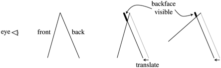
Figure 15.7 The z-bias method of silhouetting, done by translating the backface forward. If the frontface is at a different angle, as shown on the right, a different amount of the backface is visible. (Illustration after Raskar and Cohen [1460].)
Raskar and Cohen [1460, 1461] solve this neighbor dependency problem by instead fattening each backface triangle out along its edges by the amount needed to see a consistently thick line. That is, the slope of the triangle and the distance from the viewer determine how much the triangle is expanded. One method is to expand the three vertices of each triangle outward along its plane. A safer method of rendering the triangle is to move each edge of the triangle outward and connect the edges. Doing so avoids having the vertices stick far away from the original triangle. See Figure 15.8. Note that no biasing is needed with this method, as the backfaces expand beyond the edges of the frontfaces. See Figure 15.9 for results from the three methods. This fattening technique is more controllable and consistent, and has been used successfully for character outlining in video games such as Prince of Persia [1138] and Afro Samurai [250].

Figure 15.8 Triangle fattening. On the left, a backface triangle is expanded along its plane. Each edge moves a different amount in world space to make the resulting edge the same thickness in screen space. For thin triangles, this technique falls apart, as one corner becomes elongated. On the right, the triangle edges are expanded and joined to form mitered corners to avoid this problem.

Figure 15.9 Contour edges rendered with backfacing edge drawing with thick lines, z-bias, and fattened triangle algorithms. The backface edge technique gives poor joins between lines and nonuniform lines due to biasing problems on small features. The z-bias technique gives nonuniform edge width because of the dependence on the angles of the frontfaces. (Images courtesy of Raskar and Cohen [1460].)
In the method just given, the backface triangles are expanded along their original planes. Another method is to move the backfaces outward by shifting their vertices along the shared vertex normals, by an amount proportional to their z-distance from the eye [671]. This is referred to as the shell or halo method, as the shifted backfaces form a shell around the original object. Imagine a sphere. Render the sphere normally, then expand the sphere by a radius that is 5 pixels wide with respect to the sphere’s center. That is, if moving the sphere’s center one pixel is equivalent to moving it in world space by 3 millimeters, then increase the radius of the sphere by 15 millimeters. Render only this expanded version’s backfaces in black. The contour edge will be 5 pixels wide. See Figure 15.10. Moving vertices outward along their normals is a perfect task for a vertex shader. This type of expansion is sometimes called shell mapping. The method is simple to implement, efficient, robust, and gives steady performance. See Figure 15.11. A forcefield or halo effect can be made by further expanding and shading these backfaces dependent on their angle.

Figure 15.10 The triangle shell technique creates a second surface by shifting the surface along its vertex normals.

Figure 15.11 An example of real-time toon-style rendering from the game Cel Damage, using backface shell expansion to form contour edges, along with explicit crease edge drawing. (Image courtesy of Pseudo Interactive Inc.)
This shell technique has several potential pitfalls. Imagine looking head-on at a cube so that only one face is visible. Each of the four backfaces forming the contour edge will move in the direction of its corresponding cube face, so leaving gaps at the corners. This occurs because while there is a single vertex at each corner, each face has a different vertex normal. The problem is that the expanded cube does not truly form a shell, because each corner vertex is expanding in a different direction. One solution is to force vertices in the same location to share a single, new, average vertex normal. Another technique is to create degenerate geometry at the creases that then gets expanded into triangles with area. Lira et al. [1053] use an additional threshold texture to control how much each vertex is moved.
Shell and fattening techniques waste some fill, since all the backfaces are sent down the pipeline. Other limitations of all these techniques is that there is little control over the edge appearance, and semitransparent surfaces are tricky to render correctly, depending on the transparency algorithm used.
One worthwhile feature of this entire class of geometric techniques is that no connectivity information or edge lists are needed during rendering. Each triangle is processed independently from the rest, so such techniques lend themselves to GPU implementation [1461].
This class of algorithms renders only contour edges. Raskar [1461] gives a clever solution for drawing ridge crease edges on deforming models without having to create and access an edge connectivity data structure. The idea is to generate an additional polygon along each edge of the triangle being rendered. These edge polygons are bent away from the triangle’s plane by the user-defined critical dihedral angle that determines when a crease should be visible. If at any given moment two adjoining triangles are at greater than this crease angle, the edge polygons will be visible, else they will be hidden by the triangles. See Figure 15.12. Valley edges are possible with a similar technique, but require a stencil buffer and multiple passes.

Figure 15.12 A side view of two triangles joined at an edge, each with a small “fin” attached. As the two triangles bend along the edge, the fins move toward becoming visible. On the right the fins are exposed. Painted black, these appear as a ridge edge.
15.2.3 Edge Detection by Image Processing
The algorithms in the previous section are sometimes classified as image-based, as the screen resolution determines how they are performed. Another type of algorithm is more directly image-based, in that it operates entirely on data stored in image buffers and does not modify (or even directly know about) the geometry in the scene.
Saito and Takahashi [1528] first introduced this G-buffer concept, which is also used for deferred shading (Section 20.1). Decaudin [336] extended the use of G-buffers to perform toon rendering. The basic idea is simple: NPR can be done by performing image processing algorithms on various buffers of information. Many contour-edge locations can be found by looking for discontinuities in neighboring z-buffer values. Discontinuities in neighboring surface normal values often signal the location of contour and boundary edges. Rendering the scene in ambient colors or with object identification values can be used to detect material, boundary, and true silhouette edges.
Detecting and rendering these edges consists of two parts. First, the scene’s geometry is rendered, with the pixel shader saving depth, normal, object IDs, or other data as desired to various render targets. Post-processing passes are then performed, in a similar way as described in Section 12.1. A post-processing pass samples the neighborhood around each pixel and outputs a result based on these samples. For example, imagine we have a unique identification value for each object in the scene. At each pixel we could sample this ID and compare it to the four adjacent pixel ID values at the corners of our test pixel. If any of the IDs differ from the test pixel’s ID, output black, else output white. Sampling all eight neighbor pixels is more foolproof, but at a higher sampling cost. This simple kind of test can be used to draw the boundary and outline edges (true silhouettes) of most objects. Material IDs could be used to find material edges.
Contour edges can be found by using various filters on normal and depth buffers. For example, if the difference in depths between neighboring pixels is above some threshold, a contour edge is likely to exist and so the pixel is made black. Rather than a simple decision about whether the neighboring pixels match our sample, other more elaborate edge detection operators are needed. We will not discuss here the pros and cons of various edge detection filters, such as Roberts cross, Sobel, and Scharr, as the image processing literature covers these extensively [559, 1729]. Because the results of such operators are not necessarily boolean, we can adjust their thresholds or fade between black and white when in some zone. Note that the normal buffer can also detect crease edges, as a large difference between normals can signify either a contour or a crease edge. Thibault and Cavanaugh [1761] discuss how they use this technique with the depth buffer for the game Borderlands. Among other techniques, they modify the Sobel filter so that it creates single-pixel-wide outlines and the depth computation to improve precision. See Figure 15.13. It is also possible to go the other direction, adding outlines only around shadows by ignoring edges where the neighboring depths differ considerably [1138].

Figure 15.13 Modified Sobel edge detection in the game Borderlands. The final released version (not shown here) further improved the look by masking out edges for the grass in the foreground [1761]. (Images courtesy of Gearbox Software, LLC.)
The dilation operator is a type of morphological operator that is used for thickening detected edges [226, 1217]. After the edge image is generated, a separate pass is applied. At each pixel, the pixel’s value and its surrounding values to within some radius are examined. The darkest pixel value found is returned as output. In this way, a thin black line will be thickened by the diameter of the area searched. Multiple passes can be applied to further thicken lines, the trade-off being that the cost of the additional pass is offset by needing considerably fewer samples for each pass. Different results can have different thicknesses, e.g., the silhouette edges could be made thicker than the other contour edges. The related erosion operator can be used for thinning lines or other effects. See Figure 15.14 for some results.

Figure 15.14 The normal map (upper left) and depth map (upper middle) have Sobel edge detection applied to their values, with results shown in the lower left and lower middle, respectively. The image in the upper right is a thickened composite using dilation. The final rendering in the lower right is made by shading the image with Gooch shading and compositing in the edges. (Images courtesy of Drew Card and Jason L. Mitchell, ATI Technologies Inc.)
This type of algorithm has several advantages. It handles all types of surfaces, flat or curved, unlike most other techniques. Meshes do not have to be connected or even consistent, since the method is image-based.
There are relatively few flaws with this type of technique. For nearly edge-on surfaces, the z-depth comparison filter can falsely detect a contour-edge pixel across the surface. Another problem with z-depth comparison is that if the differences are minimal, then the contour edge can be missed. For example, a sheet of paper on a desk will usually have its edges missed. Similarly, the normal map filter will miss the edges of this piece of paper, since the normals are identical. This is still not foolproof; for example, a piece of paper folded onto itself will create undetectable edges where the edges overlap [725]. Lines generated show stair-step aliasing, but the various morphological antialiasing techniques described in Section 5.4.2 work well with this high-contrast output, as well as on techniques such as posterization, to improve edge quality.

Figure 15.15 Various edge methods. Feature edges such as wrinkles are part of the texture itself, added by the artist in advance. The silhouette of the character is generated with backface extrusion. The contour edges are generated using image processing edge detection, with varying weights. The left image was generated with too little weight, so these edges are faint. The middle shows outlines, on the contour edges of the nose and lips in particular. The right displays artifacts from too great a weight [250]. (Afro Samurai R & c 2006 TAKASHI OKAZAKI, GONZO / SAMURAI PROJECT. Program c 2009 BANDAI NAMCO Entertainment America Inc.)
Detection can also fail in the opposite way, creating edges where none should exist. Determining what constitutes an edge is not a foolproof operation. For example, imagine the stem of a rose, a thin cylinder. Close up, the stem normals neighboring our sample pixel do not vary all that much, so no edge is detected. As we move away from the rose, the normals will vary more rapidly from pixel to pixel, until at some point a false edge detection may occur near the edges because of these differences. Similar problems can happen with detecting edges from depth maps, with the perspective’s effect on depth being an additional factor needing compensation. Decaudin [336] gives an improved method of looking for changes by processing the gradient of the normal and depth maps rather than just the values themselves. Deciding how various pixel differences translate into color changes is a process that often needs to be tuned for the content [250, 1761]. See Figure 15.15.
Once the strokes are generated, further image processing can be performed as desired. Since the strokes can be created in a separate buffer, they can be modified on their own, then composited atop the surfaces. For example, noise functions can be used to fray and wobble the lines and the surfaces separately, creating small gaps between the two and giving a hand-drawn look. The heightfield of the paper can be used to affect the rendering, having solid materials such as charcoal deposited at the tops of bumps or watercolor paint pooled in the valleys. See Figure 15.16 for an example.

Figure 15.16 The fish model on the left is rendered on the right using edge detection, posterization, noise perturbation, blurring, and blending atop the paper. (Images courtesy of Autodesk, Inc.)
We have focused here on detecting edges using geometric or other non-graphical data, such as normals, depths, and IDs. Naturally, image processing techniques were developed for images, and such edge detection techniques can be applied to color buffers. One approach is called difference of Gaussians (DoG), where the image is processed twice with two different Gaussian filters and one is subtracted from the other. This edge detection method has been found to produce particularly pleasing results for NPR, used to generate images in a variety of artistic styles such as pencil shading and pastels [949, 1896, 1966].
Image post-processing operators feature prominently within many NPR techniques simulating artistic media such as watercolors and acrylic paints. There is considerable research in this area, and for interactive applications much of the challenge is in trying to do the most with the fewest number of texture samples. Bilateral, mean-shift, and Kuwahara filters can be used on the GPU for preserving edges and smoothing areas to appear as if painted [58, 948]. Kyprianidis et al. [949] provide a thorough review and a taxonomy of image processing effects for the field. The work by Montesdeoca et al. [1237] is a fine example of combining a number of straightforward techniques into a watercolor effect that runs at interactive rates. A model rendered with a watercolor style is shown in Figure 15.17.

Figure 15.17 On the left, a standard realistic render. On the right, the watercolor style softens textures through mean-shift color matching, and increases contrast and saturation, among other techniques. (Watercolor image courtesy of Autodesk, Inc.)
15.2.4 Geometric Contour Edge Detection
A problem with the approaches given so far is that the stylization of the edges is limited at best. We cannot easily make the lines look dashed, let alone look hand-drawn or like brush strokes. For this sort of operation, we need to find the contour edges and render them directly. Having separate, independent edge entities makes it possible to create other effects, such as having the contours jump in surprise while the mesh is frozen in shock.
A contour edge is one in which one of the two neighboring triangles faces toward the viewer and the other faces away. The test is
(15.1)
where n0 and n1 are the two triangle normals and v is the view direction from the eye to the edge (i.e., to either endpoint). For this test to work correctly, the surface must be consistently oriented (Section 16.3).
The brute-force method for finding the contour edges in a model is to run through the list of edges and perform this test [1130]. Lander [972] notes that a worthwhile optimization is to identify and ignore edges that are inside planar polygons. That is, given a connected triangle mesh, if the two neighboring triangles for an edge lie in the same plane, the edge cannot possibly be a contour edge. Implementing this test on a simple clock model dropped the edge count from 444 edges to 256. Furthermore, if the model defines a solid object, concave edges can never be contour edges. Buchanan and Sousa [207] avoid the need for doing separate dot product tests for each edge by reusing the dot product test for each individual face.
Detecting contour edges each frame from scratch can be costly. If the camera view and the objects move little from frame to frame, it is reasonable to assume that the contour edges from previous frames might still be valid contour edges. Aila and Miettinen [13] associate a valid distance with each edge. This distance is how far the viewer can move and still have the contour edge maintain its state. In any solid model each separate contour always consists of a single closed curve, called a silhouette loop or, more properly, a contour loop. For contours inside the object’s bounds, some part of the loop may be obscured. Even the actual silhouette may consist of a few loops, with parts of loops being inside the outline or hidden by other surfaces. It follows that each vertex must have an even number of contour edges [23]. See Figure 15.18. Note how the loops are often quite jagged in three dimensions when following mesh edges, with the z-depth varying noticeably. If edges forming smoother curves are desired, such as for varying thickness by distance [565], additional processing can be done to interpolate among the triangle’s normals to approximate the true contour edge inside a triangle [725, 726].

Figure 15.18 Contour loops. On the left is the camera’s view of the model. The middle shows the triangles facing away from the camera in blue. A close-up of one area of the face is shown on the right. Note the complexity and how some contour loops are hidden behind the nose. (Model courtesy of Chris Landreth, images courtesy of Pierre B′enard and Aaron Hertzmann [132].)
Tracking loop locations from frame to frame can be faster than recreating loops from scratch. Markosian et al. [1125] start with a set of loops and uses a randomized search algorithm to update this set as the camera moves. Contour loops are also created and destroyed as the model changes orientation. Kalnins et al. [848] note that when two loops merge, corrective measures need to be taken or a noticeable jump from one frame to the next will be visible. They use a pixel search and “vote” algorithm to attempt to maintain contour coherence from frame to frame.
Such techniques can give serious performance increases, but can be inexact. Linear methods are exact but expensive. Hierarchical methods that use the camera to access contour edges combine speed and precision. For orthographic views of non-animated models, Gooch et al. [562] use a hierarchy of Gauss maps for determining contour edges. Sander et al. [1539] use an n-ary tree of normal cones (Section 19.3). Hertzmann and Zorin [726] use a dual-space representation of the model that allows them to impose a hierarchy on the model’s edges.
All these explicit edge detection methods are CPU intensive and have poor cache coherency, since edges forming a contour are dispersed throughout the edge list. To avoid these costs, the vertex shader can be used to detect and render contour edges [226]. The idea is to send every edge of the model down the pipeline as two triangles forming a degenerate quadrilateral, with the two adjoining triangle normals attached to each vertex. When an edge is found to be part of the contour, the quadri-lateral’s points are moved so that it is no longer degenerate (i.e., is made visible). This thin quadrilateral fin is then drawn. This technique is based on the same idea as that described for finding contour edges for shadow volume creation (Section 7.3). If the geometry shader is a part of the pipeline, these additional fin quadrilaterals do not need to be stored but can be generated on the fly [282, 299]. A naive implementation will leave chinks and gaps between the fins, which can be corrected by modifying the shape of the fin [723, 1169, 1492].
15.2.5 Hidden Line Removal
Once the contours are found, the lines are rendered. An advantage of explicitly finding the edges is that you can stylize these as pen strokes, paint strokes, or any other medium you desire. Strokes can be basic lines, textured impostors (Section 13.6.4), sets of primitives, or whatever else you wish to try.
A further complication with attempting to use geometric edges is that not all these edges are actually visible. Rendering surfaces to establish the z-buffer can mask hidden geometric edges, which may be sufficient for simple styles such as dotted lines. Cole and Finkelstein [282] extend this for quadrilaterals representing lines by sampling the z-depths along the spine of the line itself. However, with these methods each point along the line is rendered independently, so no well-defined start and end locations are known in advance. For contour loops or other edges where the line segments are meant to define brush strokes or other continuous objects, we need to know when each stroke first appears and when it disappears. Determining visibility for each line segment is known as hidden line rendering, where a set of line segments is processed for visibility and a smaller set of (possibly clipped) line segments is returned.
Northrup and Markosian [1287] attack this problem by rendering all the object’s triangles and contour edges and assigning each a different identification number. This ID buffer is read back and the visible contour edges are determined from it. These visible segments are then checked for overlaps and linked together to form smooth stroke paths. This approach works if the line segments on the screen are short, but it does not include clipping of the line segments themselves. Stylized strokes are then rendered along these reconstructed paths. The strokes themselves can be stylized in many different ways, including effects of taper, flare, wiggle, overshoot, and fading, as well as depth and distance cues. An example is shown in Figure 15.19.

Figure 15.19 An image produced using Northrup and Markosian’s hybrid technique. Contour edges are found, built into chains, and rendered as strokes. (Image courtesy of Lee Markosian.)
Cole and Finkelstein [282] present a visibility calculation method for a set of edges. They store each line segment as two world-space coordinate values. A series of passes runs a pixel shader over the whole set of segments, clipping and determining the length in pixels of each, then creating an atlas for each of these potential pixel locations and determining visibility, and then using this atlas to create visible strokes. While complex, the process is relatively fast on the GPU and provides sets of visible strokes that have known beginning and end locations.
Stylization often consists of applying one or more premade textures to line quadri-laterals. Rougier [1516] discusses a different approach, procedurally rendering dashed patterns. Each line segment accesses a texture that stores all dashed patterns desired. Each pattern is encoded as a set of commands specifying the dashed pattern along with the endcap and join types used. Using the quadrilateral’s texture coordinates, each pattern controls a series of tests by the shader for how much of the line covers the pixel at each point in the quadrilateral.
Determining the contour edges, linking them into coherent chains, and then determining visibility for each chain to form a stroke is difficult to fully parallelize. An additional problem when producing high-quality line stylization is that for the next frame each stroke will be drawn again, changing length or possibly appearing for the first time. B′enard et al. [130] present a survey of rendering methods that provide temporal coherence for strokes along edges and patterns on surfaces. This is not a solved problem and can be computationally involved, so research continues [131].
15.3 Stroke Surface Stylization
While toon rendering is a popular style to attempt to simulate, there is an infinite variety of other styles to apply to surfaces. Effects can range from modifying realistic textures [905, 969, 973] to having the algorithm procedurally generate geometric ornamentation from frame to frame [853, 1126]. In this section, we briefly survey techniques relevant to real-time rendering.
Lake et al. [966] discuss using the diffuse shading term to select which texture is used on a surface. As the diffuse term gets darker, a texture with a darker impression is used. The texture is applied with screen-space coordinates to give a hand-drawn look. To further enhance the sketched look, a paper texture is also applied in screen space to all surfaces. See Figure 15.20. A major problem with this type of algorithm is the shower door effect, where the objects look like they are viewed through patterned glass during animation. Objects feel as though they are swimming through the texture. Breslav et al. [196] maintain a two-dimensional look for the textures by determining what image transform best matches the movements of some underlying model locations. This can maintain a connection with the screen-based nature of the fill pattern while giving a stronger connection with the object.

Figure 15.20 An image generated by using a palette of textures, a paper texture, and contour edge rendering. (Reprinted by permission of Adam Lake and Carl Marshall, Intel Corporation, copyright Intel Corporation 2002.)
One solution is obvious: Apply textures directly to the surface. The challenge is that stroke-based textures need to maintain a relatively uniform stroke thickness and density to look convincing. If the texture is magnified, the strokes appear too thick; if it is minified, the strokes are either blurred away or are thin and noisy (depending on whether mipmapping is used). Praun et al. [1442] present a real-time method of generating stroke-textured mipmaps and applying these to surfaces in a smooth fashion. Doing so maintains the stroke density on the screen as the object’s distance changes. The first step is to form the textures to be used, called tonal art maps (TAMs). This is done by drawing strokes into the mipmap levels. See Figure 15.21. Klein et al. [905] use a related idea in their “art maps” to maintain stroke size for NPR textures. With these textures in place, the model is rendered by interpolating between the tones needed at each vertex. This technique results in images with a hand-drawn feel [1441]. See Figure 15.22.

Figure 15.21 Tonal art maps (TAMs). Strokes are drawn into the mipmap levels. Each mipmap level contains all the strokes from the textures to the left and above it. In this way, interpolation between mip levels and adjoining textures is smooth. (Images courtesy of Emil Praun, Princeton University.)

Figure 15.22 Two models rendered using tonal art maps (TAMs). The swatches show the lapped texture pattern used to render each. (Images courtesy of Emil Praun, Princeton University.)
Webb et al. [1858] present two extensions to TAMs that give better results, one using a volume texture, which allows the use of color, the other using a thresholding scheme, which improves antialiasing. Nuebel [1291] gives a related method of performing charcoal rendering. He uses a noise texture that also goes from dark to light along one axis. The intensity value accesses the texture along this axis. Lee et al. [1009] use TAMs and other techniques to generate impressive images that appear drawn by pencil.
With regard to strokes, many other operations are possible than those already discussed. To give a sketched effect, edges can be jittered [317, 972, 1009] or can overshoot their original locations, as seen in the upper right and lower middle images in Figure 15.1 on page 651.
Girshick et al. [538] discuss rendering strokes along the principal curve direction lines on a surface. That is, from any given point on a surface, there is a first principal direction tangent vector that points in the direction of maximum curvature. The second principal direction is the tangent vector perpendicular to this first vector and gives the direction in which the surface is least curved. These direction lines are important in the perception of a curved surface. They also have the advantage of needing to be generated only once for static models, since such strokes are independent of lighting and shading. Hertzmann and Zorin [726] discuss how to clean up and smooth out principal directions. A considerable amount of research and development has explored using these directions and other data in applying textures to arbitrary surfaces, in driving simulation animations, and in other applications. See the report by Vaxman et al. [1814] as a starting point.
The idea of graftals [372, 853, 1126] is that geometry or decal textures can be added as needed to a surface to produce a particular effect. They can be controlled by the level of detail needed, by the surface’s orientation to the eye, or by other factors. These can also be used to simulate pen or brush strokes. An example is shown in Figure 15.23. Geometric graftals are a form of procedural modeling [407].

Figure 15.23 Two different graftal styles render the Stanford bunny. (Images courtesy of Bruce Gooch and Matt Kaplan, University of Utah.)
This chapter has only barely touched on a few of the directions NPR research has taken. See the “Further Reading and Resources” section at the end for where to go for more information. In this field there is often little or no underlying physically correct answer that we can use as a ground truth. This is both problematic and liberating. Techniques give trade-offs between speed and quality, as well as cost of implementation. Under the tight time constraints of interactive rendering rates, most schemes will bend and break under certain conditions. Determining what works well, or well enough, within your application is what makes the field a fascinating challenge. Much of our focus has been on a specific topic, contour edge detection and rendering. To conclude, we will turn our attention to lines and text. These two non-photorealistic primitives find frequent use and have some challenges of their own, so deserve separate coverage.
15.4 Lines
Rendering of simple solid “hard” lines is often considered relatively uninteresting. However, they are important in fields such as CAD for seeing underlying model facets and discerning an object’s shape. They are also useful in highlighting a selected object and in areas such as technical illustration. In addition, some of the techniques involved are applicable to other problems.
15.4.1 Triangle Edge Rendering
Correctly rendering edges on top of filled triangles is more difficult than it first appears. If a line is at exactly the same location as a triangle, how do we ensure that the line is always rendered in front? One simple solution is to render all lines with a fixed bias [724]. That is, each line is rendered slightly closer than it should truly be, so that it will be above the surface. If the fixed bias is too large, parts of edges that should be hidden appear, spoiling the effect. If the bias is too little, triangle surfaces that are nearly edge-on can hide part or all of the edges. As mentioned in Section 15.2.2, API calls such as OpenGL’s glPolygonOffset can be used to move backward the surfaces beneath the lines, based on their slopes. This method works reasonably well, but not perfectly.
A scheme by Herrell et al. [724] avoids biasing altogether. It uses a series of steps to mark and clear a stencil buffer, so that edges are drawn atop triangles correctly. This method is impractical for any but the smallest sets of triangles, as each triangle must be drawn separately and the stencil buffer cleared for each, making the process extremely time consuming.
Bærentzen et al. [86, 1295] present a method that maps well to the GPU. They employ a pixel shader that uses the triangle’s barycentric coordinates to determine the distance to the closest edge. If the pixel is close to an edge, it is drawn with the edge color. Edge thickness can be any value desired and can be affected by distance or held constant. See Figure 15.24. The main drawback is that contour edges are drawn half as thick as interior lines, since each triangle draws half of each line’s thickness. In practice this mismatch is often not noticeable.

Figure 15.24 Pixel-shader-generated lines. On the left are antialiased single-pixel width edges; on the right are variable thickness lines with haloing. (Images courtesy of J. Andreas Bærentzen.)
This idea is extended and simplified by Celes and Abraham [242], who also give a thorough summary of previous work. Their idea is to use a one-dimensional set of texture coordinates for each triangle edge, 1.0 for the two vertices defining the edge and 0.0 for the other vertex. They exploit texture mapping and the mip chain to give a constant-width edge. This approach is easy to code and provides some useful controls. For example, a maximum density can be set so that dense meshes do not become entirely filled with edges and so become a solid color.
15.4.2 Rendering Obscured Lines
In normal wireframe drawing, where no surfaces are drawn, all edges of a model are visible. To avoid drawing the lines that are hidden by surfaces, draw all the filled triangles into just the z-buffer, then draw the edges normally [1192]. If you cannot draw all surfaces before drawing all lines, a slightly more costly solution is to draw the surfaces with a solid color that matches the background.
Lines can also be drawn as partially obscured instead of fully hidden. For example, hidden lines could appear in light gray instead of not being drawn at all. This can be done by setting the z-buffer’s state appropriately. Draw as before, then reverse the sense of the z-buffer, so that only lines that are beyond the current pixel’s z-depth are drawn. Also turn off z-buffer modification, so that these drawn lines do not change any depth values. Draw the lines again in the obscured style. Only lines that would be hidden are then drawn. For stylized versions of lines, a full hidden-line-removal process can be used [282].
15.4.3 Haloing
When two lines cross, a common convention is to erase a part of the more distant line, making the ordering obvious. This can be accomplished relatively easily by drawing each line twice, once with a halo [1192]. This method erases the overlap by drawing over it in the background color. First, draw all the lines to the z-buffer, representing each line as a thick quadrilateral that represents the halo. A geometry shader can help with creating such quadrilaterals. Then, draw every line normally in color. The areas masked off by the z-buffer draws will hide lines drawn behind them. A bias or other method has to be used to ensure that each thin black line lies atop the thick z-buffer quadrilateral.
Lines meeting at a vertex can become partially hidden by the competing halos. Shortening the quadrilaterals creating the halos can help, but can lead to other artifacts. The line rendering technique from Bærentzen et al. [86, 1295] can also be used for haloing. See Figure 15.24. The halos are generated per triangle, so there are no interference problems. Another approach is to use image post-processing (Section 15.2.3) to detect and draw the halos.
Figure 15.25 shows results for some of the different line rendering methods discussed here.

Figure 15.25 Four line rendering styles. From left to right: wireframe, hidden line, obscured line, and haloed line.
15.5 Text Rendering
Given how critical reading text is to civilization, it is unsurprising that considerable attention has been lavished on rendering it well. Unlike many other objects, a single pixel change can make a significant difference, such as turning an “l” into a “1.” This section summarizes the major algorithmic approaches used for text rendering.
The eye is more sensitive to differences in intensity than to those in color. This fact has been used since at least the days of the Apple II [527] to improve perceived spatial resolution. One application of this idea is Microsoft’s ClearType technology, which is built upon one of the characteristics of liquid-crystal display (LCD) displays. Each pixel on an LCD display consists of three vertical colored rectangles, red, green, and blue—use a magnifying glass on an LCD monitor and see for yourself. Disregarding the colors of these subpixel rectangles, this configuration provides three times as much horizontal resolution as there are pixels. Using different shades fills in different subpixels, and so this technique is sometimes called subpixel rendering. The eye blends these colors together, and the reddish and blue fringes become undetectable. See Figure 15.26. This technology was first announced in 1998 and was a great help on large, low-DPI LCD monitors. Microsoft stopped using ClearType in Word 2013, evidently because of problems from blending text with different background colors. Excel uses the technology, as do various web browsers, along with Adobe’s CoolType, Apple’s Quartz 2D, and libraries such as FreeType and SubLCD. An old yet thorough article by Shemanarev [1618] covers the various subtleties and issues with this approach.

Figure 15.26 Magnified grayscale antialiased and subpixel antialiased versions of the same word. When a colored pixel is displayed on an LCD screen, the corresponding colored vertical subpixel rectangles making up the pixel are lit. Doing so provides additional horizontal spatial resolution. (Images generated by Steve Gibson’s “Free & Clear” program.)
This technique is a sterling example of how much effort is spent on rendering text clearly. Characters in a font, called glyphs, typically are described by a series of line segments and quadratic or cubic B′ezier curves. See Figure 17.9 on page 726 for an example. All font rendering systems work to determine how a glyph affects the pixels it overlaps. Libraries such as FreeType and Anti-Grain Geometry work by generating a small texture for each glyph and reusing them as needed. Different textures are made for each font size and emphasis, i.e., italics or bold.
These systems assume that each texture is pixel-aligned, one texel per pixel, as it normally is for documents. When text is applied to three-dimensional surfaces, these assumptions may no longer hold. Using a texture with a set of glyphs is a simple and popular approach, but there are some potential drawbacks. The application may still align text to face the viewer, but scaling and rotation will break the assumption of a single texel per pixel. Even if screen-aligned, font hinting may not be taken into account. Hinting is the process of adjusting the glyph’s outline to match up with the pixel cells. For example, the vertical stem of an “I” that is a texel wide is best rendered covering a single column of pixels instead of half-covering two adjacent columns. See Figure 15.27. All these factors mean a raster texture can display blurriness or aliasing problems. Rougier [1515] gives thorough coverage of the issues involved with texture-generation algorithms and shows how FreeType’s hinting can be used in an OpenGL-based glyph-rendering system.

Figure 15.27 The Verdana font rendered unhinted (top) and hinted (bottom). (Image courtesy of Nicolas Rougier [1515].)
The Pathfinder library [1834] is a recent effort that uses the GPU to generate glyphs. It has a low setup time and minimal memory use, and outperforms competing CPU-based engines. It uses tessellation and compute shaders to generate and sum up the effects of curves on each pixel, with fallbacks to geometry shaders and OpenCL on less-capable GPUs. Like FreeType, these glyphs are cached and reused. Its high-quality antialiasing, combined with the use of high-density displays, makes hinting nearly obsolete.
Applying text to arbitrary surfaces at different sizes and orientations can be done without elaborate GPU support, while still providing reasonable antialiasing. Green [580] presents such a system, first used by Valve in Team Fortress 2. The algorithm uses the sampled distance field data structure introduced by Frisken et al. [495]. Each texel holds the signed distance to the nearest edge of a glyph. A distance field attempts to encode the exact bounds of each glyph in a texture description. Bilinear interpolation then gives a good approximation of the alpha coverage of the letter at each sample. See Figure 15.28 for an example. Sharp corners may become smoothed by bilinear interpolation, but can be preserved by encoding more distance values in four separate channels [263]. A limitation of this method is that these signed distance textures are time consuming to create, so they need to be precomputed and stored. Nonetheless, several font rendering libraries are based on this technique [1440], and it adapts well to mobile devices [3]. Reshetov and Luebke [1485] summarize work along these lines and give their own scheme, based on adjusting texture coordinates for samples during magnification.

Figure 15.28 Vector textures. On the left, the letter “g” shown in its distance field representation [3]. On the right, the “no trespassing” sign is rendered from distance fields. The outline around the text is added by mapping a particular distance range to the outline color [580]. (Image on left courtesy of ARM Ltd. Image on right from “Team Fortress 2,” courtesy of Valve Corp.)
Even without scaling and rotation concerns, fonts for languages using Chinese characters, for example, may need thousands or more glyphs. A high-quality large character would require a larger texture. Anisotropic filtering of the texture may be needed if the glyph is viewed at an angle. Rendering the glyph directly from its edge and curve description would avoid the need for arbitrarily large textures and avoid the artifacts that come from sampling grids. The Loop-Blinn method [1068, 1069] uses a pixel shader to directly evaluate B′ezier curves, and is discussed in Section 17.1.2. This technique requires a tessellation step, which can be expensive when done at load time. Dobbie [360] avoids the issue by drawing a rectangle for the bounding box of each character and evaluating all the glyph outlines in a single pass. Lengyel [1028] presents a robust evaluator for whether a point is inside a glyph, which is critical to avoid artifacts, and discusses evaluation optimizations and effects such as glows, drop shadows, and multiple colors (e.g., for emojis).
Further Reading and Resources
For inspiration about non-photorealistic and toon rendering, read Scott McCloud’s Understanding Comics [1157]. For a view from a researcher’s perspective, see Hertzmann’s article [728] on using NPR techniques to help build scientific theories about art and illustration.
The book Advanced Graphics Programming Using OpenGL [1192], despite being written during the era of fixed-function hardware, has worthwhile chapters on a wide range of technical illustration and scientific visualization techniques. Though also somewhat dated, the books by the Gooches [563] and by Strothotte [1719] are good starting places for NPR algorithms. Surveys of contour edge and stroke rendering techniques are provided by Isenberg et al. [799] and Hertzmann [727]. The lectures from the SIGGRAPH 2008 course by Rusinkiewicz et al. [1521] also examine stroke rendering in detail, including newer work, and B′enard et al. [130] survey frame-to-frame coherence algorithms. For artistic image-processing effects, we refer the interested reader to the overview by Kyprianidis et al. [949]. The proceedings of the International Symposium on Non-Photorealistic Animation and Rendering (NPAR) focus on research in the field.
Mitchell et al. [1223] provide a case study about how engineers and artists collaborated to give a distinctive graphic style to the game Team Fortress 2. Shodhan and Willmott [1632] discuss the post-processing system in the game Spore and include pixel shaders for oil paint, old film, and other effects. The SIGGRAPH 2010 course “Stylized Rendering in Games” is another worthwhile source for practical examples. In particular, Thibault and Cavanaugh [1761] show the evolution of the art style for Borderlands and describe the technical challenges along the way. Evans’ presentation [446] is a fascinating exploration of a wide range of rendering and modeling techniques to achieve a particular media style.
Pranckeviˇcius [1440] provides a survey of accelerated text rendering techniques filled with links to resources.