10 Local Illumination

Search in book...
Toggle Font Controls
Create new playlist

Name your new playlist

Playlist description (optional)
Sign In

Email address

Password

Forgot Password?

or

Continue with Facebook

Continue with Google
Sign Up

Full Name

Email address

Confirm Email Address

Password

or

Continue with Facebook

Continue with Google

“Light makes right.”

—Andrew Glassner

In Chapter 9 we discussed the theory of physically based materials, and how to evaluate them with punctual light sources. With this content we can perform shading computations by simulating how lights interact with surfaces, in order to measure how much radiance is sent in a given direction to our virtual camera. This spectral radiance is the scene-referred pixel color that will be converted (Section 8.2) to the display-referred color a given pixel will have in the final image.

In reality, the interactions that we need to consider are never punctual. We have seen in Section 9.13.1 how, in order to correctly evaluate shading, we have to solve the integral of the surface BRDF response over the entire pixel footprint, which is the projection of the pixel area onto the surface. This process of integration can also be thought as an antialiasing solution. Instead of sampling a shading function that does not have a bound on its frequency components, we pre-integrate.

Up to this point, the effects of only point and directional light sources have been presented, which limits surfaces to receive light from a handful of discrete directions. This description of lighting is incomplete. In reality, surfaces receive light from all incoming directions. Outdoors scenes are not just lit by the sun. If that were true, all surfaces in shadow or facing away from the sun would be black. The sky is an important source of light, caused by sunlight scattering from the atmosphere. The importance of sky light can be seen by looking at a picture of the moon, which lacks sky light because it has no atmosphere. See Figure 10.1.

Figure 10.1. Image taken on the moon, which has no sky light due to the lack of an atmosphere to scatter sunlight. This image shows what a scene looks like when it is lit by only a direct light source. Note the pitch-black shadows and lack of any detail on surfaces facing away from the sun. This photograph shows Astronaut James B. Irwin next to the Lunar Roving Vehicle during the Apollo 15 mission. The shadow in the foreground is from the Lunar Module. Photograph taken by Astronaut David R. Scott, Commander. (Image from NASA’s collection.)

On overcast days, and at dusk or dawn, outdoor lighting is all sky light. Even on a clear day, the sun subtends a cone when seen from the earth, so is not infinitesimally small. Curiously, the sun and the moon both subtend similar angles, around half a degree, despite their enormous size difference—the sun is two orders of magnitude larger in radius than the moon.

In reality, lighting is never punctual. Infinitesimal entities are useful in some situations as cheap approximations, or as building blocks for more complete models. In order to form a more realistic lighting model, we need to integrate the BRDF response over the full hemisphere of incident directions on the surface. In real-time rendering we prefer to solve the integrals that the rendering equation (Section 11.1) entails by finding closed-form solutions or approximations of these. We usually avoid averaging multiple samples (rays), as this approach tends to be much slower. See Figure 10.2.

Figure 10.2. On the left, the integrals we have seen in Chapter 9: surface area and punctual light. On the right, the objective of this chapter will be to extend our shading mathematics to account for the integral over the light surface.

This chapter is dedicated to the exploration of such solutions. In particular, we want to extend our shading model by computing the BRDF with a variety of non-punctual light sources. Often, in order to find inexpensive solutions (or any at all), we will need to approximate the light emitter, the BRDF, or both. It is important to evaluate the final shading results in a perceptual framework, understanding what elements matter most in the final image and so allocate more effort toward these.

We start this chapter with formulae to integrate analytic area light sources. Such emit ters are the principal lights in the scene, responsible for most of the direct lighting intensity, so for these we need to retain all of our chosen material properties. Shadows should be computed for such emitters, as light leaks will result in obvious artifacts. We then investigate ways to represent more general lighting environments, ones that consist of arbitrary distributions over the incoming hemisphere. We typically accept more approximated solutions in these cases. Environment lighting is used for large, complex, but also less intense sources of light. Examples include light scattered from the sky and clouds, indirect light bouncing off large objects in the scene, and dimmer direct area light sources. Such emitters are important for the correct balance of the image that would otherwise appear too dark. Even if we consider the effect of indirect light sources, we are still not in the realm of global illumination (Chapter 11), which depends on the explicit knowledge of other surfaces in the scene.

10.1 Area Light Sources

In Chapter 9 we described idealized, infinitesimal light sources: punctual and directional. Figure 10.3 shows the incident hemisphere on a surface point, and the difference between an infinitesimal source and an area light source with a nonzero size. The light source on the left uses the definitions discussed in Section 9.4. It illuminates the surface from a single direction lc $l_{c}$ . Its brightness is represented by its color clight $c_{l} i g h t$ , defined as the reflected radiance from a white Lambertian surface facing toward the light. The point or directional light’s contribution to the outgoing radiance Lo(v) $L_{o} (v)$ in direction v $v$ is πf(lc,v)clight(n⋅lc)+ $π f (l_{c}, v) c_{l} i g h t {(n \cdot l_{c})}^{+}$ (note the x+ $x^{+}$ notation for clamping negative numbers to zero, introduced in Section 1.2). Alternatively, the brightness of the area light source (on the right) is represented by its radiance Ll $L_{l}$ . The area light subtends a solid angle ωl $ω_{l}$ from the surface location. Its contribution to the outgoing radiance in direction v $v$ is the integral of f(l,v)Ll(n⋅l)+ $f (l, v) L_{l} {(n \cdot l)}^{+}$ over ωl $ω_{l}$ .

Figure 10.3. A surface illuminated by a light source, considering the hemisphere of possible incoming light directions defined by the surface normal n $n$ . On the left, the light source is infinitesimal. On the right, it is modeled as an area light source.

The fundamental approximation behind infinitesimal light sources is expressed in the following equation:

(10.1)

L o (v) = \int l \in ω l f (l, v) L l (n \cdot l) + d l \approx π f (l c, v) c l i g h t (n \cdot l c) + .

$\begin{matrix} L_{o} (v) = \int_{l \in ω_{l}} f (l, v) L_{l} {(n \cdot l)}^{+} d l \approx π f (l_{c}, v) c_{l} i g h t {(n \cdot l_{c})}^{+} . \end{matrix}$

The amount that an area light source contributes to the illumination of a surface location is a function of both its radiance (Ll $L_{l}$ ) and its size as seen from that location (ωl $ω_{l}$ ). As we have seen in Section 9.4, point and directional light sources are approximations that cannot be realized in practice since their zero solid angle implies an infinite radiance. Understanding the visual errors that are introduced by the approximation will help to know when to use it, and what approach to take when it cannot be used. These errors will depend on two factors: how large the light source is, measured by the solid angle it covers from the shaded point, and how glossy the surface is.

Figure 10.4 shows how the specular highlight size and shape on a surface depends on both the material roughness and the size of the light source. For a small light source, one that subtends a tiny solid angle compared to the view angle, the error is small. Rough surfaces also tend to show the effect of the light source size less than polished ones. In general, both the area light emission toward a surface point and the specular lobe of the surface BRDF are spherical functions. If we consider the set of directions where the contributions of these two functions are significant, we obtain two solid angles. The determining factor in the error is proportional to the relative size of the emission angle compared to the size of the BRDF specular highlight solid angle.

Figure 10.4. From left to right, the material of the sphere increases in surface roughness, using the GGX BRDF. The rightmost image replicates the first in the series, flipped vertically. Notice how the highlight and shading caused by a large disk light on a low-roughness material can look similar to the highlight caused by a smaller light source on a much rougher material.

Finally, note that the highlight from an area light can be approximated by using a punctual light and increasing the surface roughness. This observation is useful for deriving less-costly approximations to the area light integral. It also explains why in practice many real-time rendering system produce plausible results using only punctual sources: Artists compensate for the error. However, doing so is detrimental, as it couples material properties with the particular lighting setup. Content created this way will not look right when the lighting scenario is altered.

For the special case of Lambertian surfaces, using a point light for an area light can be exact. For such surfaces, the outgoing radiance is proportional to the irradiance:

(10.2)

L o (v) = ρ s s π E,

$\begin{matrix} L_{o} (v) = \frac{ρ_{s} s}{π} E, \end{matrix}$

where ρss $ρ_{s} s$ is the subsurface albedo, or diffuse color, of the surface (Section 9.9.1). This relationship lets us use the equivalent of Equation 10.1 for computing irradiance, which is much simpler:

(10.3)

E = \int l \in ω l L l (n \cdot l) + d l \approx π c l i g h t (n \cdot l c) + .

$\begin{matrix} E = \int_{l \in ω_{l}} L_{l} {(n \cdot l)}^{+} d l \approx π c_{l} i g h t {(n \cdot l_{c})}^{+} . \end{matrix}$

The concept of vector irradiance is useful to understand how irradiance behaves in the presence of area light sources. Vector irradiance was introduced by Gershun [526], who called it the light vector, and further extended by Arvo [73]. Using vector irradiance, an area light source of arbitrary size and shape can be accurately converted into a point or directional light source.

Imagine a distribution of radiance Li $L_{i}$ coming into a point p $p$ in space. See Figure 10.5. We will assume for now that Li $L_{i}$ is wavelength-independent and thus can be represented as a scalar. For every infinitesimal solid angle dl $d l$ centered on an incoming direction l $l$ , a vector is constructed that is aligned with l $l$ and has a length equal to the (scalar) radiance incoming from that direction times dl $d l$ . Finally, all these vectors are summed to produce the vector irradiance e $e$ :

(10.4)

e (p) = \int l \in Θ L i (p, l) l d l,

$\begin{matrix} e (p) = \int_{l \in Θ} L_{i} (p, l) l d l, \end{matrix}$

where Θ $Θ$ indicates that the integral is performed over the entire sphere of directions.

Figure 10.5. Computation of vector irradiance. Left: point p $p$ is surrounded by light sources of various shapes, sizes, and radiance distributions. The brightness of the yellow color indicates the amount of radiance emitted. The orange arrows are vectors pointing in all directions from which there is any incoming radiance, and each length is equal to the amount of radiance coming from that direction times the infinitesimal solid angle covered by the arrow. In principle there should be an infinite number of arrows. Right: the vector irradiance (large orange arrow) is the sum of all these vectors. The vector irradiance can be used to compute the net irradiance of any plane at point p $p$ .

The vector irradiance e $e$ can be used to find the net irradiance at p $p$ through a plane of any orientation by performing a dot product:

(10.5)

E (p, n) - E (p, - n) = n \cdot e (p),

$\begin{matrix} E (p, n) - E (p, - n) = n \cdot e (p), \end{matrix}$

where n $n$ is the normal to the plane. The net irradiance through a plane is the difference between the irradiance flowing through the “positive side” of the plane (defined by the plane normal n $n$ ) and that flowing through the “negative side.” By itself, the net irradiance is not useful for shading. However, if no radiance is emitted through the “negative side” (in other words, the light distribution being analyzed has no parts for which the angle between l $l$ and n $n$ exceeds 90∘ $90^{\circ}$ ), then E(p,−n)=0 $E (p, - n) = 0$ and

(10.6)

E (p, n) = n \cdot e (p) .

$\begin{matrix} E (p, n) = n \cdot e (p) . \end{matrix}$

The vector irradiance of a single area light source can be used with Equation 10.6 to light Lambertian surfaces with any normal n $n$ , as long as n $n$ does not face more than 90∘ $90^{\circ}$ away from any part of the area light source. See Figure 10.6.

Figure 10.6. Vector irradiance of a single area light source. On the left, the arrows represent the vectors used to compute the vector irradiance. On the right, the large orange arrow is the vector irradiance e $e$ . The red dashed lines represent the extent of the light source, and the red vectors (each perpendicular to one of the red dashed lines) define the limits of the set of surface normals. Normals outside this set will have an angle greater than 90∘ $90^{\circ}$ with some part of the area light source. Such normals cannot use e $e$ to compute their irradiance correctly.

If our assumption that Li $L_{i}$ is wavelength-independent does not hold, then in the general case we can no longer define a single vector e $e$ . However, colored lights often have the same relative spectral distribution at all points, which means that we can factor Li $L_{i}$ into a color c′ $c^{'}$ and a wavelength-independent radiance distribution L′i $L_{i}^{'}$ . In this case we can compute e $e$ for L′i $L_{i}^{'}$ and extend Equation 10.6 by multiplying n⋅e $n \cdot e$ by c′ $c^{'}$ . Doing so results in the same equation used to compute the irradiance from a directional light source, with the following substitutions:

(10.7)

l c [2 p t] c l i g h t = e ( p ) | | e ( p ) | |, = c' | | e ( p ) | | π .

$\begin{matrix} \begin{matrix} l_{c} & = \frac{e (p)}{| | e (p) | |}, \\ [2 p t] c_{l} i g h t & = c^{'} \frac{| | e (p) | |}{π} . \end{matrix} \end{matrix}$

We have effectively converted an area light source of arbitrary shape and size to a directional light source—without introducing any error.

Equation 10.4 for finding the vector irradiance can be solved analytically for simple cases. For example, imagine a spherical light source with a center at pl $p_{l}$ and a radius rl $r_{l}$ . The light emits a constant radiance Ll $L_{l}$ from every point on the sphere, in all directions. For such a light source, Equations 10.4 and 10.7 yield the following:

(10.8)

l c c l i g h t = p l - p | | p l - p | |, = r 2 l | | p l - p | | 2 L l .

$\begin{matrix} \begin{matrix} l_{c} & = \frac{p_{l} - p}{| | p_{l} - p | |}, \\ c_{l} i g h t & = \frac{r_{l}^{2}}{| | p_{l} - p {| |}^{2}} L_{l} . \end{matrix} \end{matrix}$

This equation is the same as an omni light (Section 5.2.2) with clight0=Ll $c_{l i g h t_{0}} = L_{l}$ , r0=rl $r_{0} = r_{l}$ , and the standard inverse square distance falloff ¹ function. This falloff function can be adjusted to account for points inside the sphere, and to bound the light influence to a given maximum distance. More details on such adjustments can be found in Section 5.2.2.

All this is correct only if there is no “negative side” irradiance. Another way to think about it is that no parts of the area light source can be “under the horizon,” or occluded by the surface. We can generalize this statement. For Lambertian surfaces, all disparities between area and point light sources result from occlusion differences. The irradiance from a point light source obeys a cosine law for all normals for which the light is not occluded. Snyder derived an analytic expression for a spherical light source, taking occlusion into account [1671]. This expression is quite complex. However, since it depends on only two quantities (r/rl $r / r_{l}$ and θi $θ_{i}$ , the angle between n $n$ and lc $l_{c}$ ), it can be precomputed into a two-dimensional texture. Snyder also gives two functional approximations that are amenable for real-time rendering.

In Figure 10.4 we saw that the effects of area lighting are less noticeable for rough surfaces. This observation allows us also to use a less physically based but still effective method for modeling the effects of area lights on Lambertian surfaces: wrap lighting. In this technique, some simple modification is done to the value of n⋅l $n \cdot l$ before it is clamped to 0. One form of wrap lighting is given by Forsyth [487]:

(10.9)

E = π c l i g h t (( n \cdot l ) + k Wrap 1 + k Wrap) +,

$\begin{matrix} E = π c_{l} i g h t {(\frac{(n \cdot l) + k_{Wrap}}{1 + k_{Wrap}})}^{+}, \end{matrix}$

where kWrap $k_{Wrap}$ ranges from 0, for point light sources, to 1, for area light sources covering the entire hemisphere. Another form that mimics the effect of a large area light source is used by Valve [1222]:

(10.10)

E = π c l i g h t (( n \cdot l ) + 1 2) 2 .

$\begin{matrix} E = π c_{l} i g h t {(\frac{(n \cdot l) + 1}{2})}^{2} . \end{matrix}$

In general, if we compute area lighting, we should also modify our shadowing computations to take into account a non-punctual source. If we do not, some of the visual effect can be canceled out by the harsh shadows [193]. Soft shadows are perhaps the most visible effect of area light sources, as discussed in Chapter 7.

10.1.1. Glossy Materials

The effects of area lights on non-Lambertian surfaces are more involved. Snyder derives a solution for spherical light sources [1671], but it is limited to the original reflection-vector Phong material model and is extremely complex. In practice today approximations are needed.

The primary visual effect of area lights on glossy surfaces is the highlight. See Figure 10.4. Its size and shape are similar to the area light, while the edge of the highlight is blurred according to the roughness of the surface. This observation has led to several empirical approximations of the effect. These can be quite convincing in practice. For example, we could modify the result of our highlight calculation to incorporate a cutoff threshold that creates a large flat highlight area [606]. This can effectively create the illusion of a specular reflection from a spherical light, as in Figure 10.7.

Figure 10.7. Highlights on smooth objects are sharp reflections of the light source shape. On the left, this appearance has been approximated by thresholding the highlight value of a Blinn-Phong shader. On the right, the same object is rendered with an unmodified Blinn-Phong shader for comparison. (Image courtesy of Larry Gritz.)

Most of the practical approximations of area lighting effects for real-time rendering are based on the idea of finding, per shaded point, an equivalent punctual lighting setup that would mimic the effects of a non-infinitesimal light source. This methodology is often used in real-time rendering to solve a variety of problems. It is the same principle we saw in Chapter 9 when dealing with BRDF integrals over the pixel footprint of a surface. It yields approximations that are usually inexpensive, as all the work is done by altering the inputs to the shading equation without introducing any extra complexity. Because the mathematics is not otherwise altered, we can often guarantee that, under certain conditions, we revert to evaluating the original shading, thus preserving all its properties. Since most of a typical system’s shading code is based on punctual lights, using these for area lights introduces only localized code changes.

One of the first approximations developed is Mittring’s roughness modification used in the Unreal Engine’s “Elemental demo” [1229]. The idea is to first find a cone that contains most of the light source irradiance onto the hemisphere of directions incident to the surface. We then fit a similar cone around the specular lobe, containing “most” of the BRDF. See Figure 10.8. Both cones are then stand-ins for functions on the hemisphere, and they encompass the set of directions where these two functions have values greater than a given, arbitrary cutoff threshold. Having done so, we can approximate the convolution between the light source and the material BRDF by finding a new BRDF lobe, of a different roughness, that has a corresponding cone whose solid angle is equal to the sum of the light lobe angle and the material one.

Figure 10.8. The GGX BRDF, and a cone fitted to enclose the set of directions where the specular lobe reflects most of the incoming light radiance.

Karis [861] shows an application of Mittring’s principle to the GGX/Trowbridge-Reitz BRDF (Section 9.8.1) and a spherical area light, resulting in a simple modification of the GGX roughness parameter αg $α_{g}$ :

α' g = (α g + r l 2 | | p l - p | |) + .

$\begin{matrix} α_{g}^{'} = {(α_{g} + \frac{r_{l}}{2 | | p_{l} - p | |})}^{+} . \end{matrix}$

Note the use of the notation x+ $x^{+}$ , introduced in Section 1.2, for clamping between 0 and 1. This approximation works reasonably well and is extremely inexpensive, but breaks down for shiny, almost mirror-like materials. This failure occurs because the specular lobe is always smooth and cannot mimic the highlight caused by a sharp reflection of an area light source onto a surface. Also, most microfacet BRDF models have a lobe that are not “compact” (localized) but exhibit a wide falloff (specular tail), making roughness remapping less effective. See Figure 10.9.

Figure 10.9. Spherical lighting. From left to right: reference solution computed by numerical integration, roughness modification technique, and representative point technique. (Image courtesy of Brian Karis, Epic Games Inc.)

Instead of varying the material roughness, another idea is to represent the area illumination’s source with a light direction that changes based on the point being shaded. This is called a most representative point solution, modifying the light vector so it is in the direction of the point on the area light surface that generates the greatest energy contribution toward the shaded surface. See Figure 10.9. Picott [1415] uses the point on the light that creates the smallest angle to the reflection ray. Karis [861] improves on Picott’s formulation by approximating, for efficiency, the point of smallest angle with the point on the sphere that is at the shortest distance to the reflection ray. He also presents an inexpensive formula to scale the light’s intensity to try to preserve the overall emitted energy. See Figure 10.10.

Figure 10.10. Karis representative point approximation for spheres. First, the point on the reflection ray closest to the sphere center l $l$ is computed: pcr=(l⋅r)r−l $p_{cr} = (l \cdot r) r - l$ . The point on the sphere surface closest to pcr $p_{cr}$ is then pcs=l+pcr⋅min(1,radius||pcr||) $p_{cs} = l + p_{cr} \cdot min (1, \frac{radius}{| | p_{cr} | |})$ .

Most representative point solutions are convenient and have been developed for a variety of light geometries, so it is important to understand their theoretical background. These approaches resemble the idea of importance sampling in Monte Carlo integration, where we numerically compute the value of a definite integral by averaging samples over the integration domain. In order to do so more efficiently, we can try to prioritize samples that have a large contribution to the overall average.

A more stringent justification of their effectiveness lies in the mean value theorem of definite integrals, which allows us to replace the integral of a function with a single evaluation of the same function:

(10.11)

\int D f (x) d x = f (c) \int D 1 .

$\begin{matrix} \int_{D} f (x) d x = f (c) \int_{D} 1 . \end{matrix}$

If f(x) is continuous in D, then ∫D1 $\int_{D} 1$ is the area of the domain, with the point c∈D $c \in D$ lying on the line between the function minimum and maximum in D. For lighting, the integral we consider is the product of the BRDF and the light irradiance over the area of the hemisphere covered by the light. We usually consider our lights to be irradiating uniformly, so we need to consider only light falloff, and most approximations also assume the domain area D to be fully visible from the shaded point. Even with these assumptions, determining the point c and the normalization factor ∫D1 $\int_{D} 1$ can still be too expensive, so further approximations are employed.

Representative point solutions can also be framed by the effect they have on the shape of the highlight. On a portion of a surface where the representative point does not change because the reflection vector is outside the cone of directions subtended by the area light, we are effectively lighting with a point light. The shape of the highlight then depends only on the underlying shape of the specular lobe. Alternatively, if we are shading points on the surface where the reflection vector hits the area light, then the representative point will continuously change in order to point toward the direction of maximum contribution. Doing so effectively extends the specular lobe peak, “widening” it, an effect that is similar to the hard thresholding of Figure 10.7.

This wide, constant highlight peak is also one of the remaining sources of error in the approximation. On rougher surfaces the area light reflection looks “sharper” than the ground-truth solution (i.e., obtained via Monte Carlo integration)—an opposite visual defect to the excessive blur of the roughness modification technique. To address this, Iwanicki and Pesce [807] develop approximations obtained by fitting BRDF lobes, soft thresholds, representative point parameters, and scaling factors (for energy conservation) to spherical area lighting results computed via numerical integration. These fitted functions result in a table of parameters that are indexed by material roughness, sphere radius, and the angle between the light source center and the surface normal and view vectors. As it is expensive to directly use such multi-dimensional lookup tables in a shader, closed-form approximations are provided. Recently, de Carpentier [231] derived an improved formulation to better preserve the shape of the highlight from a spherical area source at grazing angles for microfacet-based BRDFs. This method works by finding a representative point that maximizes n⋅h $n \cdot h$ , the dot product between the surface normal and the light-view half vector, instead of n⋅r $n \cdot r$ of the original formulation (which was derived for the Phong BRDF).

10.1.2. General Light Shapes

So far we have seen a few ways to compute shading from uniformly emitting spherical area lights and arbitrary glossy BRDFs. Most of these methods employ various approximations in order to arrive at mathematical formulae that are fast to evaluate in real time, and thus display varying degrees of error when compared to a ground-truth solution of the problem. However, even if we had the computational power to derive an exact solution, we would still be committing a large error, one that we embedded in the assumptions of our lighting model. Real-world lights usually are not spheres, and they hardly would be perfect uniform emitters. See Figure 10.11. Spherical area lights are still useful in practice, because they provide the simplest way to break the erroneous correlation between lighting and surface roughness that punctual lights introduce. However, spherical sources are typically a good approximation of most real light fixtures only if these are relatively small.

Figure 10.11. Commonly used light shapes. From left to right: sphere, rectangle (card), tube (line), and a tube with focused emission (concentrated along the light surface normal, not evenly spread in the hemisphere). Note the different highlights they create.

As the objective of physically based real-time rendering is to generate convincing, plausible images, there is only so far that we can go in this pursuit by limiting ourselves to an idealized scenario. This is a recurring trade-off in computer graphics. We can usually choose between generating accurate solutions to easier problems that make simplifying assumptions or deriving approximate solutions to more general problems that model reality more closely.

One of the simplest extensions to spherical lights are “tube” lights (also called “capsules”), which can be useful to represent real-world fluorescent tube lights. See Figure 10.12. For Lambertian BRDFs, Picott [1415] shows a closed-form formula of the lighting integral, which is equivalent to evaluating the lighting from two point lights at the extremes of the linear light segment with an appropriate falloff function:

(10.12)

\int p 1 p 0 (n \cdot x | | x | |) 1 | | x | | 2 d x = n \cdot p 0 | | p 0 | | 2 + n \cdot p 1 | | p 1 | | 2 | | p 0 | | | | p 1 | | + ( p 0 \cdot p 1 ),

$\begin{matrix} \int_{p_{0}}^{p_{1}} (n \cdot \frac{x}{| | x | |}) \frac{1}{{| | x | |}^{2}} d x = \frac{\frac{n \cdot p_{0}}{| | p_{0} {| |}^{2}} + \frac{n \cdot p_{1}}{| | p_{1} {| |}^{2}}}{| | p_{0} | | | | p_{1} | | + (p_{0} \cdot p_{1})}, \end{matrix}$

where p0 $p_{0}$ and p1 $p_{1}$ are the two endpoints of the linear light and n $n$ is the surface normal. Picott also derives a representative point solution for the integral with a Phong specular BRDF, approximating it as the lighting from a point light placed at the position on the light segment that, when joined to the surface point under consideration, forms the smallest angle to the reflection vector. This representative point solution dynamically transforms the linear light into a point one, so we can then use any approximation for spherical light to “thicken” the light fixture into a capsule.

As in the case of spherical lights, Karis [861] presents a more efficient (but somewhat less accurate) variant on Picott’s original solution, by using the point on the line with the smallest distance to the reflection vector (instead of the smallest angle), and presents a scaling formula in an attempt to restore energy conservation.

Representative point approximations for many other light shapes could be obtained fairly easily, such as for rings and Bézier segments, but we usually do not want to branch our shaders too much. Good light shapes are ones that can be used to represent many real-world lights in our scenes. One of the most expressive classes of shapes are planar area lights, defined as a section of a plane bound by a given geometrical shape, e.g., a rectangle (in which case they are also called card lights), a disk, or more generally a polygon. These primitives can be used for emissive panels such as billboards and television screens, to stand in for commonly employed photographic lighting (softboxes, bounce cards), to model the aperture of many more complex lighting fixtures, or to represent lighting reflecting from walls and other large surfaces in a scene.

One of the first practical approximations to card lights (and disks, as well) was derived by Drobot [380]. This again is a representative point solution, but it is particularly notable both because of the complexity of extending this methodology to two-dimensional areas of a plane, and for the overall approach to the solution. Drobot starts from the mean value theorem and, as a first approximation, determines that a good candidate point for light evaluation should lie near the global maximum of the lighting integral.

For a Lambert BRDF, this integral is

(10.13)

L l \int l \in ω l (n \cdot l) + 1 r 2 l d l,

$\begin{matrix} L_{l} \int_{l \in ω_{l}} {(n \cdot l)}^{+} \frac{1}{r_{l}^{2}} d l, \end{matrix}$

where Ll $L_{l}$ is the constant radiance emitted by the light, ωl $ω_{l}$ is the solid angle subtended by the light geometry, rl $r_{l}$ is the length of the ray from the surface to the light plane in the direction l $l$ , and (n⋅l)+ ${(n \cdot l)}^{+}$ is the usual Lambertian clamped dot product. The maximum of (n⋅l)+ ${(n \cdot l)}^{+}$ is the point pc $p_{c}$ on the boundary of the light region that is closest to the point p′ $p^{'}$ found by intersecting a ray originating from the surface, in the direction of the normal, with the light plane. Similarly, the maximum of 1/r2l $1 / r_{l}^{2}$ is the point pr $p_{r}$ on the boundary closest to the point p′′ $p^{″}$ that is the closest on the light plane to the surface point being shaded. See Figure 10.13.

Figure 10.13. Geometric construction of Drobot’s rectangular area light representative point approximation.

The global maximum of the integrand will then lie somewhere on the segment connecting pr $p_{r}$ and pc $p_{c}$ : pmax=tmpc+(1−tm)pr $p_{m} a x = t_{m} p_{c} + (1 - t_{m}) p_{r}$ , tm∈[0,1] $t_{m} \in [0, 1]$ . Drobot uses numerical integration to find the best representative point for many different configurations, and then finds a single tm $t_{m}$ that works best on average.

Drobot’s final solution employs further approximations for both diffuse and specular lighting, all motivated by comparisons with the ground-truth solution found numerically. He also derives an algorithm for the important case of textured card lights, where the emission is not assumed to be constant but is modulated by a texture, over the rectangular region of the light. This process is executed using a three-dimensional lookup table containing pre-integrated versions of the emission textures over circular footprints of varying radii. Mittring [1228] employs a similar method for glossy reflections, intersecting a reflection ray with a textured, rectangular billboard and indexing precomputed blurred version of the texture depending on the ray intersection distance. This work precedes Drobot’s developments, but is a more empirical, less principled approach that does try to match a ground-truth integral solution.

For the more general case of planar polygonal area lights, Lambert [967] originally derived an exact closed-form solution for perfectly diffuse surfaces. This method was improved by Arvo [74], allowing for glossy materials modeled as Phong specular lobes. Arvo achieves this by extending the concept of vector irradiance to higher-dimensional irradiance tensors and employing Stoke’s theorem to solve an area integral as a simpler integral along the contour of the integration domain. The only assumptions his method makes are that the light is fully visible from the shaded surface points (a common one to make, which can be circumvented by clipping the light polygon with the plane tangent to the surface) and that the BRDF is a radially symmetric cosine lobe. Unfortunately, in practice Arvo’s analytic solution is quite expensive for real-time rendering, as it requires evaluating a formula whose time complexity is linear in the exponent of the Phong lobe used, per each edge of the area light polygon. Recently Lecocq [1004] made this method more practical by finding an O(1) approximation to the contour integral function and extending the solution to general, half-vector-based BRDFs.

Figure 10.14. The key idea behind the linearly transformed cosine technique is that a simple cosine lobe (on the left) can be easily scaled, stretched, and skewed by using a 3×3 $3 \times 3$ transform matrix. This allows the cosine lobe to take many different shapes on the sphere. (Image courtesy of Eric Heitz.)

Figure 10.15. Given an LTC and a spherical polygonal domain (on the left), we can transform them both by the inverse of the LTC matrix to obtain a simple cosine lobe and new domain (on the right). The integral of the cosine lobe with the transformed domain is equal to the integral of the LTC over the original domain. (Image courtesy of Eric Heitz.)

All practical real-time area lighting methods described so far employ both certain simplifying assumptions to allow the derivation of analytic constructions and approximations to deal with the resulting integrals. Heitz et al. [711] take a different approach with linearly transformed cosines (LTCs), which yield a practical, accurate, and general technique. Their method starts with devising a category of functions on the sphere that both are highly expressive (i.e., they can take many shapes) and can be integrated easily over arbitrary spherical polygons. See Figure 10.14. LTCs use just a cosine lobe transformed by a 3×3 $3 \times 3$ matrix, so they can be resized, stretched, and rotated over the hemisphere to adapt to a variety of shapes. The integral of a simple cosine lobe (unlike Blinn-Phong, not taken to an exponent) with a spherical polygon is well established, dating back to Lambert [74,967]. The key observation Heitz et al. make is that extending the integral with a transformation matrix on the lobe does not change its complexity. We can transform the polygonal domain by the inverse of the matrix and cancel the matrix inside the integral, returning to a simple cosine lobe as the integrand. See Figure 10.15. For generic BRDFs and area light shapes, the only remaining work left is to find ways (approximations) to express the BRDF function on the sphere as one or more LTCs, work that can be done offline and tabulated in lookup arrays indexed with the BRDF parameters: roughness, incidence angle, and so on. Linearly transformed cosine-based solutions are derived both for general textured polygonal area light sources and for specialized, cheaper-to-compute shapes such as card, disk, and line lights. LTCs can be more expensive than representative point solutions, but are much more accurate.

10.2 Environment Lighting

In principle, reflectance (Equation ) does not distinguish between light arriving directly from a light source and indirect light that has been scattered from the sky or objects in the scene. All incoming directions have radiance, and the reflectance equation integrates over them all. However, in practice direct light is usually distinguished by relatively small solid angles with high radiance values, and indirect light tends to diffusely cover the rest of the hemisphere with moderate to low radiance values. This split provides good practical reasons to handle the two separately.

So far, the area light techniques discussed integrating constant radiance emitted from the light’s shape. Doing so creates for each shaded surface point a set of directions that have a constant nonzero incoming radiance. What we examine now are methods to integrate radiance defined by a varying function over all the possible incoming directions. See Figure 10.16.

Figure 10.16. Rendering of a scene under different environment lighting scenarios.

While we will generally talk about indirect and “environment” lighting here, we are not going to investigate global illumination algorithms. The key distinction is that in this chapter all the shading mathematics does not depend on the knowledge of other surfaces in the scene, but rather on a small set of light primitives. So, while we could, for example, use an area light to model the bounce of the light off a wall, which is a global effect, the shading algorithm does not need to know about the existence of the wall. The only information it has is about a light source, and all the shading is performed locally. Global illumination (Chapter 11) will often be closely related to the concepts of this chapter, as many solutions can be seen as ways to compute the right set of local light primitives to use for every object or surface location in order to simulate the interactions of light bouncing around the scene.

Ambient light is the simplest model of environment lighting, where the radiance does not vary with direction and has a constant value LA $L_{A}$ . Even such a basic model of environment lighting improves visual quality significantly. A scene with no consideration of the light indirectly bounced from objects appears highly unrealistic. Objects in shadow or facing away from the light in such a scene would be completely black, which is unlike any scene found in reality. The moonscape in Figure 10.1 on page 376 comes close, but even in such scenes some indirect light reflects off nearby objects.

The exact effects of ambient light will depend on the BRDF. For Lambertian surfaces, the fixed radiance LA $L_{A}$ results in a constant contribution to outgoing radiance, regardless of surface normal n $n$ or view direction v $v$ :

(10.14)

L o (v) = ρ s s π L A \int l \in Ω (n \cdot l) d l = ρ s s L A .

$\begin{matrix} L_{o} (v) = \frac{ρ_{s} s}{π} L_{A} \int_{l \in Ω} (n \cdot l) d l = ρ_{s} s L_{A} . \end{matrix}$

When shading, this constant outgoing radiance contribution is added to the contributions from direct light sources. For arbitrary BRDFs, the equivalent equation is

(10.15)

L o (v) = L A \int l \in Ω f (l, v) (n \cdot l) d l .

$\begin{matrix} L_{o} (v) = L_{A} \int_{l \in Ω} f (l, v) (n \cdot l) d l . \end{matrix}$

The integral in this equation is the same as the directional albedo R(v) $R (v)$ (Equation in Section 9.3), and so the equation is equivalent to Lo(v)=LAR(v) $L_{o} (v) = L_{A} R (v)$ . Older real-time rendering applications sometimes assumed a constant value for R(v) $R (v)$ , referred to as the ambient color camb $c_{amb}$ . This further simplifies the equation to Lo(v)=cambLA $L_{o} (v) = c_{amb} L_{A}$ .

The reflectance equation ignores occlusion, i.e., that many surface points will be blocked from “seeing” some of the incoming directions by other objects, or other parts of the same object. This simplification reduces realism in general, but it is particularly noticeable for ambient lighting, which appears extremely flat when occlusion is ignored. Methods for addressing this problem will be discussed in Section 11.3, and in Section 11.3.4 in particular.

10.3 Spherical and Hemispherical Functions

To extend environment lighting beyond a constant term, we need a way to represent the incoming radiance from any direction onto an object. To begin, we will consider the radiance to be a function of only the direction being integrated, not the surface position. Doing so works on the assumption that the lighting environment is infinitely far away.

Radiance arriving at a given point can be different for every incoming direction. Lighting can be red from the left and green from the right, or blocked from the top but not from the side. These types of quantities can be represented by spherical functions, which are defined over the surface of the unit sphere, or over the space of directions in R3 $R^{3}$ . We will denote this domain as S. How these functions work is not affected by whether they produce a single value or many values. For example, the same representation used for storing a scalar function can also be used to encode color values, by storing a separate scalar function for every color channel.

Assuming Lambertian surfaces, spherical functions can be used to compute environment lighting by storing a precomputed irradiance function, e.g., radiance convolved with a cosine lobe, for each possible surface normal direction. More sophisticated methods store radiance and compute the integral with a BRDF at runtime, per shaded surface point. Spherical functions are also used extensively in global illumination algorithms (Chapter 11).

Related to spherical functions are those for a hemisphere, for cases where values for only half of the directions are defined. For example, these functions are used to describe incoming radiance at a surface where there is no light coming from below.

We will refer to these representations as spherical bases, as they are bases for vector spaces of functions defined over a sphere. Even though the ambient/highlight/direction form (Section 10.3.3) is technically not a basis in the mathematical sense, we will also refer to it using this term for simplicity. Converting a function to a given representation is called projection, and evaluating the value of a function from a given representation is called reconstruction.

Each representation has its own set of trade-offs. Properties we might seek in a given basis are:

Efficient encoding (projection) and decoding (lookup).
The ability to represent arbitrary spherical functions with few coefficients and low reconstruction error.
Rotational invariance of projection, which is the result of rotating the projection of a function is the same as rotating the function and then projecting it. This equivalence means that a function approximated with, e.g., spherical harmonics will not change when rotated.
Ease of computing sums and products of encoded functions.
Ease of computing spherical integrals and convolutions.

10.3.1. Simple Tabulated Forms

The most straightforward way to represent a spherical (or hemispherical) function is to pick several directions and store a value for each. Evaluating the function involves finding some number of samples around the evaluation direction and reconstructing the value with some form of interpolation.

This representation is simple, yet expressive. Adding or multiplying such spherical functions is as easy as adding or multiplying their corresponding tabulated entries. We can encode many different spherical functions with arbitrarily low error by adding more samples as needed.

Figure 10.17. A few different ways to distribute points over the surface of a sphere. From left to right: random points, cubical grid points, and spherical t-design.

It is not trivial to distribute samples over a sphere (see Figure 10.17) in a way that allows efficient retrieval, while representing all directions relatively equally. The most commonly used technique is to first unwrap the sphere into a rectangular domain, then sample this domain with a grid of points. As a two-dimensional texture represents exactly that, a grid of points (texels) on a rectangle, we can use the texels as the underlying storage for the sample values. Doing so lets us leverage GPU-accelerated bilinear texture filtering for fast lookups (reconstruction). Later in this chapter we will discuss environment maps (Section 10.5), which are spherical functions in this form, and discuss different options for unwrapping the sphere.

Tabulated forms have downsides. At low resolutions the quality provided by the hardware filtering is often unacceptable. The computational complexity of calculating convolutions, a common operation when dealing with lighting, is proportional to the number of samples and can be prohibitive. Moreover, projection is not invariant under rotation, which can be problematic for certain applications. For example, imagine encoding the radiance of a light shining from a set of directions as it hits the surface of an object. If the object rotates, the encoded results might reconstruct differently. This can lead to variations in the amount of radiant energy encoded, which can manifest as pulsating artifacts as the scene animates. It is possible to mitigate these issues by employing carefully constructed kernel functions associated with each sample during projection and reconstruction. More commonly, though, just using a dense enough sampling is sufficient to mask these issues.

Typically, tabulated forms are employed when we need to store complex, high-frequency functions that require many data points to be encoded with low error. If we need to encode spherical functions compactly, with only a few parameters, more complex bases can be used.

A popular basis choice, an ambient cube (AC) is one of the simplest tabulated forms, constructed out of six squared cosine lobes oriented along the major axes [1193]. It is called an ambient “cube” because it is equivalent to storing data in the faces of a cube and interpolating as we move from one direction to another. For any given direction, only three of the lobes are relevant, so the parameters for the other three do not need to be fetched from memory [766]. Mathematically, the ambient cube can be defined as

(10.16)

F A C (d) = d d \cdot s e l + (c +, c -, d),

$\begin{matrix} F_{AC} (d) = d d \cdot s e l_{+} (c_{+}, c_{-}, d), \end{matrix}$

where c+ $c_{+}$ and c− $c_{-}$ contain the six values for the cube faces and sel+(c+,c−,d) $s e l_{+} (c_{+}, c_{-}, d)$ is a vector function that assumes, for each of its components, a value from c+ $c_{+}$ or c− $c_{-}$ based on whether the respective component in d $d$ is positive.

An ambient cube is similar to a cube map (Section 10.4) with a single texel on each cube face. In some systems, performing the reconstruction in software for this particular case might be faster than using the GPU’s bilinear filtering on cube maps. Sloan [1656] derives a simple formulation to convert between the ambient cube and the spherical harmonic basis (Section 10.3.2).

The quality of reconstruction using the ambient cube is fairly low. Slightly better results can be achieved by storing and interpolating eight values instead of six, corresponding to the cube vertices. More recently, an alternative called ambient dice (AD) was presented by Iwanicki and Sloan [808]. The basis is formed from squared and fourth-power cosine lobes oriented along the vertices of an icosahedron. Six out of twelve values stored are needed for reconstruction, and the logic to determine which six are retrieved is slightly more complex than the corresponding logic for ambient cubes, but the quality of the result is much higher.

10.3.2. Spherical Bases

There are an infinite number of ways to project (encode) functions onto representations that use a fixed number of values (coefficients). All we need is a mathematical expression that spans our spherical domain with some parameters we can change. We can then approximate any given function we want by fitting, i.e., finding the values of the parameters that minimize the error between our expression and the given function.

The most minimal possible choice is to use a constant:

F c (θ, ϕ) = c \cdot 1 .

$\begin{matrix} F_{c} (θ, ϕ) = c \cdot 1 . \end{matrix}$

We can derive the projection of a given function f into this basis by averaging it over the surface area of the unit sphere: c=14π∫Ωf(θ,ϕ) $c = \frac{1}{4 π} \int_{Ω} f (θ, ϕ)$ . The average c of a periodic function is also known as the DC component. This basis has the benefit of simplicity, and even respects some of the properties we are looking for (ease of reconstruction, addition, product, rotational invariance). However, it cannot express most spherical functions well, as it just replaces them with their average. We could construct a slightly more complex approximation using two coefficients, a and b:

F hemi (θ, ϕ) = a + cos ( θ ) + 1 2 (b - a),

$\begin{matrix} F_{hemi} (θ, ϕ) = a + \frac{cos (θ) + 1}{2} (b - a), \end{matrix}$

which creates a representation that can encode exact values at the poles and can interpolate between them across the surface of the sphere. This choice is more expressive, but now projection is more complicated and is not invariant for all rotations. In fact, this basis could be seen as a tabular form with only two samples, placed at the poles.

In general, when we talk about a basis of a function space, we mean that we have a set of functions whose linear combination (weighting and summing) can be used to represent other functions over a given domain. An example of this concept is shown in Figure 10.18.

Figure 10.18. A basic example of basis functions. In this case, the space is “functions that have values between 0 and 1 for inputs between 0 and 5.” The left plot shows an example of such a function. The middle plot shows a set of basis functions (each color is a different function). The right plot shows an approximation to the target function, formed by multiplying each of the basis functions by a weight and summing them. The basis functions are shown scaled by their respective weights. The black line shows the result of summing, which is an approximation to the original function, shown in gray for comparison.

The rest of this section explores some choices of bases that can be used to approximate functions on the sphere.

Spherical Radial Basis Functions

The low quality of reconstruction with tabulated forms using GPU hardware filtering is, at least to some extent, caused by the bilinear shape functions used to interpolate samples. Other functions can be used to weight samples for reconstruction. Such functions may produce higher-quality results than bilinear filtering, and they may have other advantages. One family of functions often used for this purpose are the spherical radial basis functions (SRBFs). They are radially symmetric, which makes them functions of only one argument, the angle between the axis along which they are oriented and the evaluation direction. The basis is formed by a set of such functions, called lobes, that are spread across the sphere. Representation of a function consists of a set of parameters for each of the lobes. This set can include their directions, but it makes projection much harder (requiring nonlinear, global optimization). For this reason, lobe directions are often assumed to be fixed, spread uniformly across the sphere, and other parameters are used, such as the magnitude of each lobe or its spread, i.e., the angle covered. Reconstruction is performed by evaluating all the lobes for a given direction and summing the results.

Spherical Gaussians

One particularly common choice for an SRBF lobe is a spherical Gaussian (SG), also called a von Mises-Fisher distribution in directional statistics. We should note that von-Mises-Fisher distributions usually include a normalization constant, one that we avoid in our formulation. A single lobe can be defined as

(10.17)

G (v, d, λ) = e λ (v \cdot d - 1),

$\begin{matrix} G (v, d, λ) = e^{λ (v \cdot d - 1)}, \end{matrix}$

where v $v$ is the evaluation direction (a unit vector), d $d$ is the lobe direction axis (mean of the distribution, also normalized), and λ≥0 $λ \geq 0$ is the lobe sharpness (which controls its angular width, also called the concentration parameter or spread) [1838].

To construct the spherical basis, we then use a linear combination of a given number of spherical Gaussians:

(10.18)

F G (v) = \sum k w k G (v, d k, λ k) .

$\begin{matrix} F_{G} (v) = \sum_{k} w_{k} G (v, d_{k}, λ_{k}) . \end{matrix}$

Performing the projection of a spherical function into this representation entails finding the set of parameters {wk,dk,λk} ${w_{k}, d_{k}, λ_{k}}$ that minimize the reconstruction error. This process is typically done by numerical optimization, often using a nonlinear least-squares optimization algorithm (such as Levenberg-Marquardt). Note that if we allow the complete set parameters to vary in the optimization process, we would not be using a linear combination of functions, so Equation 10.18 does not represent a basis. A proper basis is obtained only when we choose a fixed set of lobes (directions and spreads), so that the entire domain is well covered [1127], and perform projection by fitting only the weights wk $w_{k}$ . Doing so also greatly simplifies the optimization problem, as now it can be formulated as ordinary least-squares optimization. This is also a good solution if we need to interpolate between different sets of data (projected functions). For that use case, allowing the lobe directions and sharpness to vary is detrimental, as these parameters are highly nonlinear.

A strength of this representation is that many operations on SGs have simple, analytic forms. The product of two spherical Gaussians is another spherical Gaussian (see [1838]):

G 1 G 2 = G (v, d ' | | d ' | |, λ'),

$\begin{matrix} G_{1} G_{2} = G (v, \frac{d^{'}}{| | d^{'} | |}, λ^{'}), \end{matrix}$

where

d' = λ 1 d 1 + λ 2 d 2 λ 1 + λ 2, λ' = (λ 1 + λ 2) | | d' | | .

$\begin{matrix} d^{'} = \frac{λ_{1} d_{1} + λ_{2} d_{2}}{λ_{1} + λ_{2}}, λ^{'} = (λ_{1} + λ_{2}) | | d^{'} | | . \end{matrix}$

The integral of a spherical Gaussian over the sphere can also be computed analytically:

\int Ω G (v) d v = 2 π 1 - e 2 λ λ,

$\begin{matrix} \int_{Ω} G (v) d v = 2 π \frac{1 - e^{2 λ}}{λ}, \end{matrix}$

which means that the integral of the product of two spherical Gaussians also has a simple formulation.

If we can express light radiance as spherical Gaussians, then we can integrate its product with a BRDF encoded in the same representation to perform lighting calculations [1408,1838]. For these reasons, SGs have been used in many research projects [582,1838] as well as industry applications [1268].

As for Gaussian distributions on the plane, von Mises-Fisher distributions can be generalized to allow anisotropy. Xu et al. [1940] introduced anisotropic spherical Gaussians (ASGs; see Figure 10.19), which are defined by augmenting the single direction d $d$ with two supplemental axes t $t$ and b $b$ that together form an orthonormal tangent frame:

(10.19)

G (v, [d, t, b], [λ, μ]) = S (v, d) e - λ (v \cdot t) 2 - μ (v \cdot b) 2,

$\begin{matrix} G (v, [d, t, b], [λ, μ]) = S (v, d) e^{- λ {(v \cdot t)}^{2} - μ {(v \cdot b)}^{2}}, \end{matrix}$

where λ,μ≥0 $λ, μ \geq 0$ control the lobe spread along the two axis of the tangent frame and S(v,d)=(v⋅d)+ $S (v, d) = {(v \cdot d)}^{+}$ is a smoothing term. This term is the main difference between the Fisher-Bingham distribution used in orientation statistics and the ASGs we employ for computer graphics. Xu et al. also provide analytic approximations for the integral, product, and convolution operators.

While SGs have many desirable properties, one of their drawbacks is that, unlike tabulated forms and in general kernels with a limited extent (bandwidth), they have global support. Each lobe is nonzero for the entire sphere, even though its falloff is fairly quick. This global extent means that if we use N lobes to represent a function, we will need all N of them for reconstruction in any direction.

Spherical Harmonics

Spherical harmonics ² (SH) are an orthogonal set of basis functions over the sphere. An orthogonal set of basis functions is a set such that the inner product of any two different functions from the set is zero. The inner product is a more general, but similar, concept to the dot product. The inner product of two vectors is their dot product: the sum of the multiplication between pairs of components. We can similarly derive a definition of the inner product over two functions by considering the integral of these functions multiplied together:

(10.20)

⟨ f i (x), f j (x) ⟩ \equiv \int f i (x) f j (x) d x,

$\begin{matrix} ⟨ f_{i} (x), f_{j} (x) ⟩ \equiv \int f_{i} (x) f_{j} (x) d x, \end{matrix}$

where the integration is performed over the relevant domain. For the functions shown in Figure 10.18, the relevant domain is between 0 and 5 on the x-axis (note that this particular set of functions is not orthogonal). For spherical functions the form is slightly different, but the basic concept is the same:

(10.21)

⟨ f i (n), f j (n) ⟩ \equiv \int n \in Θ f i (n) f j (n) d n,

$\begin{matrix} ⟨ f_{i} (n), f_{j} (n) ⟩ \equiv \int_{n \in Θ} f_{i} (n) f_{j} (n) d n, \end{matrix}$

where n∈Θ $n \in Θ$ indicates that the integral is performed over the unit sphere.

An orthonormal set is an orthogonal set with the additional condition that the inner product of any function in the set with itself is equal to 1. More formally, the condition for a set of functions {fj()} ${f_{j} ()}$ to be orthonormal is

(10.22)

⟨ f i (), f j () ⟩ = {0, 1, where i \neq j, where i = j .

$\begin{matrix} ⟨ f_{i} (), f_{j} () ⟩ = \{\begin{matrix} 0, & where i \neq j, \\ 1, & where i = j . \end{matrix} \end{matrix}$

Figure 10.20 shows an example similar to Figure 10.18, where the basis functions are orthonormal.

Figure 10.20. Orthonormal basis functions. This example uses the same space and target function as Figure 10.18, but the basis functions have been modified to be orthonormal. The left image shows the target function, the middle shows the orthonormal set of basis functions, and the right shows the scaled basis functions. The resulting approximation to the target function is shown as a dotted black line, and the original function is shown in gray for comparison.

Note that the orthonormal basis functions shown in Figure 10.20 do not overlap. This condition is necessary for an orthonormal set of non-negative functions, as any overlap would imply a nonzero inner product. Functions that have negative values over part of their range can overlap and still form an orthonormal set. Such overlap usually leads to better approximations, since it allows the bases to be smooth. Bases with disjoint domains tend to cause discontinuities.

The advantage of an orthonormal basis is that the process to find the closest approximation to the target function is straightforward. To perform projection, the coefficient for each basis function is the inner product of the target function ftarget() $f_{target} ()$ with the appropriate basis function:

(10.23)

k j = ⟨ f t a r g e t (), f j () ⟩, f t a r g e t () \approx \sum j = 1 n k j f j () .

$\begin{matrix} \begin{matrix} k_{j} = ⟨ f_{t} a r g e t (), f_{j} () ⟩, \\ f_{t} a r g e t () \approx \sum_{j = 1}^{n} k_{j} f_{j} () . \end{matrix} \end{matrix}$

In practice this integral has to be computed numerically, typically by Monte Carlo sampling, averaging n directions distributed evenly over the sphere.

An orthonormal basis is similar in concept to the “standard basis” for three-dimensional vectors introduced in Section 4.2.4. Instead of a function, the target of the standard basis is a point’s location. The standard basis is composed of three vectors (one per dimension) instead of a set of functions. The standard basis is orthonormal by the same definition used in Equation 10.22. The method of projecting a point onto the standard basis is also the same, as the coefficients are the result of dot products between the position vector and the basis vectors. One important difference is that the standard basis exactly reproduces every point, while a finite set of basis functions only approximates its target functions. The result can never be exact because the standard basis uses three basis vectors to represent a three-dimensional space. A function space has an infinite number of dimensions, so a finite number of basis functions can never perfectly represent it.

Spherical harmonics are orthogonal and orthonormal, and they have several other advantages. They are rotationally invariant, and SH basis functions are inexpensive to evaluate. They are simple polynomials in the x-, y-, and z-coordinates of unit-length vectors. However, like spherical Gaussians, they have global support, so during reconstruction all of the basis functions need to be evaluated. The expressions for the basis functions can be found in several references, including a presentation by Sloan [1656]. His presentation is noteworthy in that it discusses many practical tips for working with spherical harmonics, including formulae and, in some cases, shader code. More recently Sloan also derived efficient ways to perform SH reconstruction [1657].

Figure 10.21. The first five frequency bands of spherical harmonics. Each spherical harmonic function has areas of positive values (colored green) and areas of negative values (colored red), fading to black as they approach zero. (Spherical harmonic visualizations courtesy of Robin Green.)

The SH basis functions are arranged in frequency bands. The first basis function is constant, the next three are linear functions that change slowly over the sphere, and the next five represent quadratic functions that change slightly faster. See Figure 10.21. Functions that are low frequency (i.e., change slowly over the sphere), such as irradiance values, are accurately represented with a relatively small number of SH coefficients (as we will see in Section 10.6.1).

When projecting to spherical harmonics, the resulting coefficients represent the amplitudes of various frequencies of the projected function, i.e., its frequency spectrum. In this spectral domain, a fundamental property holds: The integral of the product of two functions is equal to the dot product of the coefficients of the function projections. This property allows us to compute lighting integrals efficiently.

Many operations on spherical harmonics are conceptually simple, boiling down to a matrix transform on the vector of coefficients [583]. Among these operations are the important cases of computing the product of two functions projected to spherical harmonics, rotating projected functions, and computing convolutions. A matrix transform in SH in practice means the complexity of these operations is quadratic in the number of coefficients used, which can be a substantial cost. Luckily, these matrices often have peculiar structures that can be exploited to devise faster algorithms. Kautz et al. [869] present a method to optimize the rotation computations by decomposing them into rotations about the x- and z-axes. A popular method for fast rotation of low-order SH projections is given by Hable [633]. Green’s survey [583] discusses how to exploit the block structure of the rotation matrix for faster computation. Currently the state of the art is represented by a decomposition into zonal harmonics, as presented by Nowrouzezahrai et al. [1290].

A common problem of spectral transformations such as spherical harmonics and the H-basis, described below, is that they can exhibit a visual artifact called ringing (also called the Gibbs phenomenon). If the original signal contains rapid changes that cannot be represented by the band-limited approximation, the reconstruction will show oscillation. In extreme cases this reconstructed function can even generate negative values. Various prefiltering methods can be used to combat this problem [1656,1659].

Other Spherical Representations

Many other representations are possible to encode spherical functions using a finite number of coefficients. Linearly transformed cosines (Section 10.1.2) are an example of a representation that can efficiently approximate BRDF functions, while having the property of being easily integrable over polygonal sections of a sphere.

Spherical wavelets [1270,1579,1841] are a basis that balances locality in space (having compact support) and in frequency (smoothness), allowing for compressed representation of high-frequency functions. Spherical piecewise constant basis functions [1939], which partition the sphere into areas of constant value, and biclustering approximations [1723], which rely on matrix factoring, have also been used for environment lighting.

10.3.3. Hemispherical Bases

Even though the above bases can be used to represent hemispherical functions, they are wasteful. Half of the signal is always equal to zero. In these cases the use of representations constructed directly on the hemispherical domain is usually preferred. This is especially relevant for functions defined over surfaces: The BRDF, the incoming radiance, and the irradiance arriving at given point of an object are all common examples. These functions are naturally constrained to the hemisphere centered at the given surface point and aligned with the surface normal; they do not have values for directions that point inside the object.

Ambient/Highlight/Direction

One of the simplest representations along these lines is a combination of a constant function and a single direction where the signal is strongest over the hemisphere. It is usually called the ambient/highlight/direction (AHD) basis, and its most common use is to store irradiance. The name AHD denotes what the individual components represent: a constant ambient light, plus a single directional light that approximates the irradiance in the “highlight” direction, and the direction where most of the incoming light is concentrated. The AHD basis usually requires storing eight parameters. Two angles are used for the direction vector and two RGB colors for the ambient and directional light intensities. Its first notable use was in the game Quake III, where volumetric lighting for dynamic objects was stored in this way. Since then it has been used in several titles, such as those from the Call of Duty franchise.

Projection onto this representation is somewhat tricky. Because it is nonlinear, finding the optimal parameters that approximate the given input is computationally expensive. In practice, heuristics are used instead. The signal is first projected to spherical harmonics, and the optimal linear direction is used to orient the cosine lobe. Given the direction, ambient and highlight values can be computed using least-squares minimization. Iwanicki and Sloan [809] show how to perform this projection while enforcing non-negativity.

Radiosity Normal Mapping/Half-Life 2 Basis

Valve uses a novel representation, which expresses directional irradiance in the context of radiosity normal mapping, for the Half-Life 2 series of games [1193,1222]. Originally devised to store precomputed diffuse lighting while allowing for normal mapping, it is often now called the Half-Life 2 basis. It represents hemispherical functions on surfaces by sampling three directions in tangent space. See Figure 10.22.

The coordinates of the three mutually perpendicular basis vectors in tangent space are

(10.24)

m 0 = (- 1 6 - \sqrt, 1 2 - \sqrt, 1 3 - \sqrt), m 1 = (- 1 6 - \sqrt, - 1 2 - \sqrt, 1 3 - \sqrt), m 2 = (2 - \sqrt 3 - \sqrt, 0, 1 3 - \sqrt) .

$\begin{matrix} m_{0} = (\frac{- 1}{\sqrt{6}}, \frac{1}{\sqrt{2}}, \frac{1}{\sqrt{3}}), m_{1} = (\frac{- 1}{\sqrt{6}}, \frac{- 1}{\sqrt{2}}, \frac{1}{\sqrt{3}}), m_{2} = (\frac{\sqrt{2}}{\sqrt{3}}, 0, \frac{1}{\sqrt{3}}) . \end{matrix}$

For reconstruction, given the tangent-space direction d $d$ we can interpolate the values—E0 $E_{0}$ , E1 $E_{1}$ , and E2 $E_{2}$ —along the three basis vectors: ³

(10.25)

E (n) = \sum k = 0 2 max ( m k \cdot n , 0 ) 2 E k \sum k = 0 2 max ( m k \cdot n , 0 ) 2 .

$\begin{matrix} E (n) = \frac{\sum_{k = 0}^{2} max {(m_{k} \cdot n, 0)}^{2} E_{k}}{\sum_{k = 0}^{2} max {(m_{k} \cdot n, 0)}^{2}} . \end{matrix}$

Green [579] points out that Equation 10.25 can be made significantly less costly if the following three values are precomputed in the tangent-space direction d $d$ instead:

(10.26)

d k = max ( m k \cdot n , 0 ) 2 \sum k = 0 2 max ( m k \cdot n , 0 ) 2,

$\begin{matrix} d_{k} = \frac{max {(m_{k} \cdot n, 0)}^{2}}{\sum_{k = 0}^{2} max {(m_{k} \cdot n, 0)}^{2}}, \end{matrix}$

for k=0,1,2 $k = 0, 1, 2$ . Equation 10.25 then simplifies to

(10.27)

E (n) = \sum 2 k = 0 d k E k .

$\begin{matrix} E (n) = \sum_{k = 0}^{2} d_{k} E_{k} . \end{matrix}$

Green describes several other advantages to this representation, some of which are discussed in Section 11.4.

The Half-Life 2 basis works well for directional irradiance. Sloan [1654] found that this representation produces results superior to low-order hemispherical harmonics.

Hemispherical Harmonics/H-Basis

Gautron et al. [518] specialize spherical harmonics to the hemispherical domain, which they call hemispherical harmonics (HSHs). Various methods are possible to perform this specialization.

For example, Zernike polynomials are orthogonal functions like spherical harmonics, but defined on the unit disk. As with SH, these can be used to transform functions in the frequency domain (spectrum), which yields a number of convenient properties. As we can transform a unit hemisphere into a disk, we can use Zernike polynomials to express hemispherical functions [918]. However, performing reconstruction with these is quite expensive. Gautron et al.’s solution both is more economical and allows for relatively fast rotation by matrix multiplication on the vector of coefficients.

The HSH basis is still more expensive to evaluate than spherical harmonics, however, as it is constructed by shifting the negative pole of the sphere to the outer edge of the hemisphere. This shift operation makes the basis functions non-polynomial, requiring divisions and square roots to be computed, which are typically slow on GPU hardware. Moreover, the basis is always constant at the hemisphere edge as it maps to a single point on the sphere before the shifting. The approximation error can be considerable near the edges, especially if only a few coefficients (spherical harmonic bands) are used.

Habel [627] introduced the H-basis, which takes part of the spherical harmonic basis for the longitudinal parameterization and parts of the HSH for the latitudinal one. This basis, one that mixes shifted and non-shifted versions of the SH, is still orthogonal, while allowing for efficient evaluation.

10.4 Environment Mapping

Recording a spherical function in one or more images is called environment mapping, as we typically use texture mapping to implement the lookups in the table. This representation is one of the most powerful and popular forms of environment lighting. Compared to other spherical representations, it consumes more memory but is simple and fast to decode in real time. Moreover, it can express spherical signals of arbitrarily high frequency (by increasing the texture’s resolution) and accurately capture any range of environment radiance (by increasing each channel’s number of bits). Such accuracy comes at a price. Unlike the colors and shader properties stored in other commonly used textures, the radiance values stored in environment maps usually have a high dynamic range. More bits per texel mean environment maps tend to take up more space than other textures and can be slower to access.

We have a basic assumption for any global spherical function, i.e., one used for all objects in the scene, that the incoming radiance Li $L_{i}$ is dependent on only the direction. This assumption requires that the objects and lights being reflected are far away, and that the reflector does not reflect itself.

Shading techniques relying on environment mapping are typically not characterized by their ability to represent environment lighting, but by how well we can integrate them with given materials. That is, what kinds of approximations and assumptions do we have to employ on the BRDF in order to perform the integration? Reflection mapping is the most basic case of environment mapping, where we assume that the BRDF is a perfect mirror. An optically flat surface or mirror reflects an incoming ray of light to the light’s reflection direction ri $r_{i}$ (Section 9.5). Similarly, the outgoing radiance includes incoming radiance from just one direction, the reflected view vector r $r$ . This vector is computed in the same way as ri $r_{i}$ (Equation ):

(10.28)

r = 2 (n \cdot v) n - v .

$\begin{matrix} r = 2 (n \cdot v) n - v . \end{matrix}$

The reflectance equation for mirrors is greatly simplified:

(10.29)

L o (v) = F (n, r) L i (r),

$\begin{matrix} L_{o} (v) = F (n, r) L_{i} (r), \end{matrix}$

where F is the Fresnel term (Section 9.5). Note that unlike the Fresnel terms in half vector-based BRDFs (which use the angle between the half vector h $h$ and l $l$ or v $v$ ), the Fresnel term in Equation 10.29 uses the angle between the surface normal n $n$ and the reflection vector r $r$ (which is the same as the angle between n $n$ and v $v$ ).

Since the incoming radiance Li $L_{i}$ is dependent on only the direction, it can be stored in a two-dimensional table. This representation enables us to efficiently light a mirror-like surface of any shape with an arbitrary incoming radiance distribution. We do so by computing r $r$ for each point and looking up the radiance in the table. This table is called an environment map, as introduced by Blinn and Newell [158]. See Figure 10.23.

Figure 10.23. Reflection mapping. The viewer sees an object, and the reflected view vector r $r$ is computed from v $v$ and n $n$ . The reflected view vector accesses the environment’s representation. The access information is computed by using some projector function to convert the reflected view vector’s (x, y, z) to a texture coordinate that is used to retrieve the store radiance of the environment.

The steps of a reflection mapping algorithm are:

Generate or load a texture representing the environment.
For each pixel that contains a reflective object, compute the normal at the location on the surface of the object.
Compute the reflected view vector from the view vector and the normal.
Use the reflected view vector to compute an index into the environment map that represents the incoming radiance in the reflected view direction.
Use the texel data from the environment map as incoming radiance in Equation 10.29.

A potential stumbling block of environment mapping is worth mentioning. Flat surfaces usually do not work well when environment mapping is used. The problem with a flat surface is that the rays that reflect off of it usually do not vary by more than a few degrees. This tight clustering results in a small part of the environment table being mapped onto a relatively large surface. Techniques that also use positional information of where the radiance is emitted from, discussed in Section 11.6.1, can give better results. Also, if we assume completely flat surfaces, such as floors, real-time techniques for planar reflections (Section 11.6.2) may be used.

The idea of illuminating a scene with texture data is also known as image-based lighting (IBL), typically when the environment map is obtained from real-world scenes using cameras capturing 360 degree panoramic, high dynamic range images [332,1479].

Using environment mapping with normal mapping is particularly effective, yielding rich visuals. See Figure 10.24. This combination of features is also historically important. A restricted form of bumped environment mapping was the first use of a dependent texture read (Section 6.2) in consumer-level graphics hardware, giving rise to this ability as a part of the pixel shader.

There are a variety of projector functions that map the reflected view vector into one or more textures. We discuss the more popular mappings here, noting the strengths of each.

10.4.1. Latitude-Longitude Mapping

In 1976, Blinn and Newell [158] developed the first environment mapping algorithm. The mapping they used is the familiar latitude/longitude system used on a globe of the earth, which is why this technique is commonly referred to as latitude-longitude mapping or lat-long mapping. Instead of being like a globe viewed from the outside, their scheme is like a map of the constellations in the night sky. Just as the information on a globe can be flattened to a Mercator or other projection map, an environment surrounding a point in space can be mapped to a texture. When a reflected view vector is computed for a particular surface location, the vector is converted to spherical coordinates (ρ,ϕ) $(ρ, ϕ)$ . Here $ϕ$ , equivalent to the longitude, varies from 0 to $2 π$ radians, and $ρ$ , the latitude, varies from 0 to $π$ radians. The pair $(ρ, ϕ)$ is computed from Equation 10.30, where $r = (r_{x}, r_{y}, r_{z})$ is the normalized reflected view vector, with $+ z$ being up:

Figure 10.24. A light (at the camera) combined with bump and environment mapping. Left to right: no environment mapping, no bump mapping, no light at the camera, and all three combined. (Images generated from the three.js example webgl_materials_displacementmap [218], model from AMD GPU MeshMapper.)

(10.30)

$\begin{matrix} ρ = arccos (r_{z}) and ϕ = atan 2 (r_{y}, r_{x}) . \end{matrix}$

See page 8 for a description of atan2. These values are then used to access the environment map and retrieve the color seen in the reflected view direction. Note that latitude-longitude mapping is not identical to the Mercator projection. It keeps the distance between latitude lines constant, while Mercator goes to infinity at the poles.

Figure 10.25. The earth with equally spaced latitude and longitude lines, as opposed to the traditional Mercator projection. (Image from NASA’s “Blue Marble” collection.)

Some distortion is always necessary to unwrap a sphere into a plane, especially if we do not allow multiple cuts, and each projection has its own trade-offs between preserving area, distances, and local angles. One problem with this mapping is that the density of information is nowhere near uniform. As can be seen in the extreme stretching in the top and bottom parts of Figure 10.25, the areas near the poles receive many more texels than those near the equator. This distortion is problematic not only because it does not result in the most efficient encoding, but it can also result in artifacts when employing hardware texture filtering, especially visible at the two pole singularities. The filtering kernel does not follow the stretching of the texture, thus effectively shrinking in areas that have a higher texel density. Note also that while the projection mathematics is simple, it might not be efficient, as transcendental functions such as arccosine are costly on GPUs.

10.4.2. Sphere Mapping

Initially mentioned by Williams [1889], and independently developed by Miller and Hoffman [1212], sphere mapping was the first environment mapping technique supported in general commercial graphics hardware. The texture image is derived from the appearance of the environment as viewed orthographically in a perfectly reflective sphere, so this texture is called a sphere map. One way to make a sphere map of a real environment is to take a photograph of a shiny sphere, such as a Christmas tree ornament. See Figure 10.26.

Figure 10.26. A sphere map (left) and the equivalent map in latitude-longitude format (right).

The resulting circular image is also called a light probe, as it captures the lighting situation at the sphere’s location. Photographing spherical probes can be an effective method to capture image-based lighting, even if we use other encodings at runtime. We can always convert between a spherical projection and another form, such as the cube mapping discussed later (Section 10.4.3), if the capture has enough resolution to overcome the differences in distortion between methods.

A reflective sphere shows the entire environment on just the front of the sphere. It maps each reflected view direction to a point on the two-dimensional image of this sphere. Say we wanted to go the other direction, that, given a point on the sphere map, we would want the reflected view direction. To do this, we would take the surface normal on the sphere at that point, and then generate the reflected view direction. So, to reverse the process and get the location on the sphere from the reflected view vector, we need to derive the surface normal on the sphere, which will then yield the (u, v) parameters needed to access the sphere map.

The sphere’s normal is the half-angle vector between the reflected view vector $r$ and the original view vector $v$ , which is (0, 0, 1) in the sphere map’s space. See Figure 10.27.

Figure 10.27. Given the constant view direction $v$ and reflected view vector $r$ in the sphere map’s space, the sphere map’s normal $n$ is halfway between the two. For a unit sphere at the origin, the intersection point $h$ has the same coordinates as the unit normal $n$ . Also shown is how $h_{y}$ (measured from the origin) and the sphere map texture coordinate v (not to be confused with the view vector $v$ ) are related.

This normal vector $n$ is the sum of the original and reflected view vectors, i.e., $(r_{x}, r_{y}, r_{z} + 1)$ . Normalizing this vector gives the unit normal:

(10.31)

$\begin{matrix} n = (\frac{r_{x}}{m}, \frac{r_{y}}{m}, \frac{r_{z} + 1}{m}), where m = \sqrt{r_{x}^{2} + r_{y}^{2} + {(r_{z} + 1)}^{2}} . \end{matrix}$

If the sphere is at the origin and its radius is 1, then the unit normal’s coordinates are also the location $h$ of the normal on the sphere. We do not need $h_{z}$ , as $(h_{x}, h_{y})$ describes a point on the image of the sphere, with each value in the range $[- 1, 1]$ . To map this coordinate to the range [0, 1) to access the sphere map, divide each by two and add a half:

(10.32)

$\begin{matrix} m = \sqrt{r_{x}^{2} + r_{y}^{2} + {(r_{z} + 1)}^{2}}, u = \frac{r_{x}}{2 m} + 0.5, and v = \frac{r_{y}}{2 m} + 0.5 . \end{matrix}$

In contrast to latitude-longitude mapping, sphere mapping is much simpler to compute and shows one singularity, located around the edge of the image circle. The drawback is that the sphere map texture captures a view of the environment that is valid for only a single view direction. This texture does capture the entire environment, so it is possible to compute the texture coordinates for a new viewing direction. However, doing so can result in visual artifacts, as small parts of the sphere map become magnified due to the new view, and the singularity around the edge becomes noticeable. In practice, the sphere map is commonly assumed to follow the camera, operating in view space.

Since sphere maps are defined for a fixed view direction, in principle each point on a sphere map defines not just a reflection direction, but also a surface normal. See Figure 10.27. The reflectance equation can be solved for an arbitrary isotropic BRDF, and its result can be stored in a sphere map. This BRDF can include diffuse, specular, retroreflective, and other terms. As long as the illumination and view directions are fixed, the sphere map will be correct. Even a photographic image of a real sphere under actual illumination can be used, as long as the BRDF of the sphere is uniform and isotropic.

It is also possible to index two sphere maps, one with the reflection vector and another with the surface normal, to simulate specular and diffuse environment effects. If we modulate the values stored in the sphere maps to account for the color and roughness of the surface material, we have an inexpensive technique that can generate convincing (albeit view-independent) material effects. This method was popularized by the sculpting software Pixologic ZBrush as “MatCap” shading. See Figure 10.28.

Figure 10.28. Example of “MatCap” rendering. The objects on the left are shaded using the two sphere maps on the right. The map at the top is indexed using the view-space normal vector, while the bottom one uses the view-space reflection vector, and the values from both are added together. The resulting effect is quite convincing, but moving the viewpoint would reveal that the lighting environment follows the coordinate frame of the camera.

10.4.3. Cube Mapping

In 1986, Greene [590] introduced the cubic environment map, usually called a cube map. This method is far and away the most popular method today, and its projection is implemented directly in hardware on modern GPUs. The cube map is created by projecting the environment onto the sides of a cube positioned with its center at the camera’s location. The images on the cube’s faces are then used as the environment map. See Figures 10.29 and 10.30. A cube map is often visualized in a “cross” diagram, i.e., opening the cube and flattening it onto a plane. However, on hardware cube maps are stored as six square textures, not as a single rectangular one, so there is no wasted space.

Figure 10.29. Illustration of Greene’s environment map, with key points shown. The cube on the left is unfolded into the environment map on the right.

Figure 10.30. The same environment map used in Figure 10.26, transformed to the cube map format.

It is possible to create cube maps synthetically by rendering a scene six times with the camera at the center of the cube, looking at each cube face with a $90^{\circ}$ view angle. See Figure 10.31. To generate cube maps from real-world environments, usually spherical panoramas acquired by stitching or specialized cameras are projected into the cube map coordinate system.

Figure 10.31. The environment map lighting in Forza Motorsport 7 updates as the cars change position.

Cubic environment mapping is view-independent, unlike sphere mapping. It also has much more uniform sampling characteristics than latitude-longitude mapping, which oversamples the poles compared to the equator. Wan et al. [1835,1836] present a mapping called the isocube that has an even lower sampling-rate discrepancy than cube mapping, while still leveraging the cube mapping texture hardwarefor performance.

Accessing the cube map is straightforward. Any vector can be used directly as a three-component texture coordinate to fetch data in the direction it is pointing. So, for reflections we can just pass the reflected view vector $r$ to the GPU, without even needing to normalize it. On older GPUs, bilinear filtering could reveal seams along the cube edges, as the texture hardware was unable to properly filter across different cube faces (an operation that is somewhat expensive to perform). Techniques to sidestep this issue were developed, such as making the view projections a bit wider so that a single face would also contain these neighboring texels. All modern GPUs can now correctly perform this filtering across edges, so these methods are nolonger necessary.

10.4.4. Other Projections

Today the cube map is the most popular tabular representation for environment lighting, due to its versatility, accuracy in reproducing high-frequency details, and execution speed on the GPU. However, a few other projections have been developed that are worth mentioning.

Heidrich and Seidel [702,704] propose using two textures to perform dual paraboloid environment mapping. The idea is like that of sphere mapping, but instead of generating the texture by recording the reflection of the environment off a sphere, two parabolic projections are used. Each paraboloid creates a circular texture similar to a sphere map, with each covering an environment hemisphere.

As with sphere mapping, the reflected view ray is computed in the map’s basis, i.e., in its frame of reference. The sign of the z-component of the reflected view vector is used to decide which of the two textures to access. The access function is

(10.33)

$\begin{matrix} u = \frac{r_{x}}{2 (1 + r_{z})} + 0.5, v = \frac{r_{y}}{2 (1 + r_{z})} + 0.5 \end{matrix}$

for the front image, and the same, with sign reversals for $r_{z}$ , for the back image.

The parabolic map has more uniform texel sampling of the environment compared to the sphere map, and even to the cube map. However, care has to be taken for proper sampling and interpolation at the seam between the two projections, which makes accessing a dual paraboloid map more expensive.

Octahedral mapping [434] is another noteworthy projection. Instead of mapping the surrounding sphere to a cube, it is mapped to an octahedron (see Figure 10.32). To flatten this geometry into textures, its eight triangular faces are cut and arranged on a flat plane. Either a square or a rectangular configuration is possible. If we use the square configuration, the mathematics for accessing an octahedral map is quite efficient.

Figure 10.32. Cube map unwrapping of a sphere (left) compared to octahedral unwrapping (right). (After a Shadertoy by Nimitz.)

Given a reflection direction $r$ , we compute a normalized version using the absolute value $L_{1}$ norm:

$\begin{matrix} r^{'} = \frac{r}{| r_{x} | + | r_{y} | + | r_{z} |} . \end{matrix}$

For the case where $r_{y}^{'}$ is positive, we can then index the square texture with

(10.34)

$\begin{matrix} u = r_{x}^{'} \cdot 0.5 + 0.5, v = r_{y}^{'} \cdot 0.5 + 0.5 . \end{matrix}$

Where $r_{y}^{'}$ is negative, we need to “fold” the second half of the octahedron outward with the transform

(10.35)

$\begin{matrix} u = (1 - | r_{z}^{'} |) \cdot s i g n (r_{x}^{'}) \cdot 0.5 + 0.5, v = (1 - | r_{x}^{'} |) \cdot s i g n (r_{z}^{'}) \cdot 0.5 + 0.5 . \end{matrix}$

The octahedral mapping does not suffer from the filtering issues of the dual paraboloid mapping, as the seams of the parameterization correspond with the edges of the texture used. Texture “wrap-around” sampling modes can automatically access texels from the other side and perform the correct interpolation. Though the mathematics for the projection is slightly more involved, in practice performance is better. The amount of distortion introduced is similar to that for cube maps, so octahedral maps can be a good alternative when cube map texture hardware is not present. Another notable use is as a way of expressing three-dimensional directions (normalized vectors) using only two coordinates, as a mean of compression (Section 16.6).

For the special case of environment maps that are radially symmetric around an axis, Stone [1705] proposes a simple factorization using a single one-dimensional texture storing the radiance values along any meridian line from the symmetry axis. He extends this scheme to two-dimensional textures, storing in each row an environment map pre-convolved with a different Phong lobe. This encoding can simulate a variety of materials, and was employed to encode radiance emitted from a clear sky.

10.5 Specular Image-Based Lighting

While environment mapping was originally developed as a technique for rendering mirror-like surfaces, it can be extended to glossy reflections as well. When used to simulate general specular effects for infinitely distant light sources, environment maps are also known as specular light probes. This term is used because they capture the radiance from all directions at a given point in the scene (thus probing), and use that information to evaluate general BRDFs—not only the restricted cases of pure mirrors or Lambertian surfaces. The name specular cube maps also is used for the common case of storing the environment lighting in cube maps that have been manipulated to simulate reflections on glossy materials.

To simulate surface roughness, the environment’s representation in the texture can be prefiltered [590]. By blurring the environment map texture, we can present a specular reflection that looks rougher than perfectly mirror-like reflection. Such blurring should be done in a nonlinear fashion, i.e., different parts of the texture should be blurred differently. This adjustment is needed because environment map texture representations have a nonlinear mapping to the ideal spherical space of directions. The angular distance between the centers of two adjacent texels is not constant, nor is the solid angle covered by a single texel. Specialized tools to preprocess cube maps, such as AMD’s CubeMapGen (now open source), take these factors into account when filtering. Neighboring samples from other faces are used to create the mipmap chain, and the angular extent of each texel is factored in. Figure 10.33 shows an example.

Figure 10.33. On the top, the original environment map (left) and shading results applied on a sphere (right). On the bottom, the same environment map blurred with a Gaussian kernel emulates the appearance of a rough material.

Blurring the environment map, while empirically approaching the look of rough surfaces, bears no connection with an actual BRDF. A more principled method is to consider the shape a BRDF function takes on the sphere when a given surface normal and view direction are taken in consideration. We then filter the environment map using this distribution. See Figure 10.34.

Figure 10.34. The left figure shows an eye ray reflecting off an object to retrieve a perfect mirror reflection from an environment texture (a cube map in this case). The right figure shows a reflected view ray’s specular lobe, which is used to sample the environment texture. The green square represents a cross section of the cube map, and the red tick marks denote the boundaries between texels.

Filtering an environment map with a specular lobe is not trivial, as a BRDF can assume any shape, depending on its roughness parameters along with the view and normal vectors. There are at least five dimensions of input values (roughness and two polar angles each for the view and normal directions) that control the resulting lobe shape. Storing several environment maps for each choice among these is infeasible.

10.5.1. Prefiltered Environment Mapping

Practical implementations of prefiltering for environment lighting applied to glossy materials require approximations to the BRDF used so that the resulting texture is independent of the view and normal vectors. If we restrict the shape variation of the BRDF to only the material glossiness, we can compute and store a few environment maps corresponding to different choices of the roughness parameter, and chose the appropriate one to use at runtime. In practice, this means restricting the blur kernels we use, and thus the lobe shapes, to be radially symmetric around the reflection vector.

Imagine some light coming in from near a given reflected view direction. Light directly from the reflected view direction will give the largest contribution, dropping off as the direction to the incoming light increasingly differs from the reflected view direction. The area of the environment map texel multiplied by the texel’s BRDF contribution gives the relative effect of this texel. This weighted contribution is multiplied by the color of the environment map texel, and the results are summed to compute $q$ . The sum of the weighted contributions, s, is also computed. The final result, $q / s$ , is the overall color integrated over the reflected view direction’s lobe and is stored in the resulting reflection map.

If we use the Phong material model, the radial symmetry assumption naturally holds, and we can compute environment lighting almost exactly. Phong [1414] derived his model empirically and, in contrast to the BRDFs we have seen in Section 9.8, there is no physical motivation. Both Phong’s model and the Blinn-Phong [159] BRDF we discussed in Section 9.8.1 are cosine lobes raised to a power, but in the case of Phong shading, the cosine is formed by the dot product of the reflection (Equation ) and view vectors, instead of the half vector (see Equation ) and the normal. This causes the reflection lobe to be rotationally symmetrical. See Figure on page 338.

With a radially symmetric specular lobe, the only effect for which we still cannot accommodate, as it makes the lobe shape dependent on the view direction, is horizon clipping. Think about viewing a shiny (not mirror) sphere. Looking near the center of the sphere’s surface gives, say, a symmetric Phong lobe. Viewing the surface near the sphere’s silhouette must in reality have a piece of its lobe cut off, as no light from below the horizon can reach the eye. See Figure 10.35. This is the same issue we saw previously when discussing approximations for area lighting (Section 10.1), and in practice it is often ignored by real-time methods. Doing so can cause excessively bright shading at grazing angles.

Figure 10.35. A shiny sphere is seen by two viewers. Separate locations on the sphere give the same reflected view direction for both viewers. The left viewer’s surface reflection samples a symmetric lobe. The right viewer’s reflection lobe must be chopped off by the horizon of the surface itself, since light cannot reflect off the surface below its horizon.

Heidrich and Seidel [704] use a single reflection map in this way to simulate the blurriness of a surface. To accommodate for different roughness levels, it is common to employ the mipmaps (Section 6.2.2) of an environment cube map. Each level is used to store blurred versions of the incoming radiance, with higher mip levels storing rougher surfaces, i.e., wider Phong lobes [80,582,1150,1151]. During runtime, we can address the cube map by using the reflection vector and forcing the selection of a given mip level based on the desired Phong exponent (material roughness). See Figure 10.36.

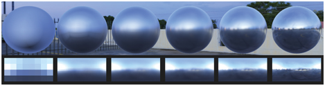
Figure 10.36. Environment map prefiltering. A cube map has been convolved with GGX lobes of varying roughness, and the results are stored in the texture mip chain. With the roughness decreasing from left to right, the resulting texture mips are displayed at the bottom and a sphere is rendered above accessing them in the direction of the reflection vector.

Wider filter areas used by rougher materials remove high frequencies and so require less resolution for adequate results, which maps perfectly to the mipmap structure. Moreover, by employing the GPU hardware’s trilinear filtering, it is possible to sample in between prefiltered mip levels, simulating roughness values for which we do not have exact representations. When combined with a Fresnel term, such reflection maps work plausibly well for glossy surfaces. For performance and aliasing reasons, the selection of the mipmap level to use should take into consideration not only the material roughness at the shaded point, but also the change in normal and roughness over the surface area covered by the screen pixel footprint being shaded. Ashikhmin and Ghosh [80] point out that, for best results, the indices of the two candidate mipmap levels (the minification level computed by the texturing hardware and the level corresponding to the current filter width) should be compared, and the index of the lower-resolution mipmap level should be used. To be more accurate, the widening effect of the surface variance should be taken into account, and a new roughness level, corresponding to a BRDF lobe that best fits the average of lobes in the pixel footprint, should be employed. This problem is exactly the same as BRDF antialiasing (Section 9.13.1), and the same solutions apply.

The filtering scheme presented earlier assumes that all lobes for a given reflected view direction are the same shape and height. This assumption also means that the lobes have to be radially symmetric. Beyond the problem at the horizon, most BRDFs do not have uniform, radially symmetric lobes at all angles. For example, at grazing angles the lobes often become sharper and thinner. Also, the lengths of the lobes normally vary with elevation angle

This effect is not usually perceivable for curved surfaces. However, for flat surfaces such as floors, radially symmetric filters can introduce noticeable errors. (See Figure on page 338)

Convolving the Environment Map

Generating prefiltered environment maps means computing for every texel, corresponding to a direction $v$ , the integral of the environment radiance with the specular lobe D:

$\begin{matrix} \int_{Ω} D (l, v) L_{i} (l) d l . \end{matrix}$

This integral is a spherical convolution, and in general cannot be performed analytically, as $L_{i}$ , for environment maps, is known only in tabular form. A popular numerical solution is to adopt Monte Carlo methods:

(10.36)

$\begin{matrix} \int_{Ω} D (l, v) L_{i} (l) d l \approx lim_{N \to \infty} \frac{1}{N} \sum_{k = 1}^{N} \frac{D (l_{k}, v) L_{i} (l_{k})}{p (l_{k}, v)}, \end{matrix}$

where $l_{k}$ for $k = 1, 2, \dots, N$ are discrete samples over the unit sphere (directions), and $p (l_{k}, v)$ is the probability function associated with generating a sample in the direction $l_{k}$ . If we sample the sphere uniformly, then $p (l_{k}, v) = 1$ always. While this summation is correct for each direction $v$ that we want to integrate, when storing the results in a environment map we also have to take into account the distortion that the projection imposes, by weighting each computed texel by the solid angle it subtends (see Driscoll [376]).

While Monte Carlo methods are simple and correct, they might take a large number of samples to converge to the numerical value of the integral, which can be slow even for an offline process. This situation is especially true for the first levels of the mipmap, where we encode shallow specular lobes (high exponents in the case of Blinn-Phong, low roughness for Cook-Torrance). We not only have more texels to compute (as we need the resolution to store high-frequency details), but also the lobe might be nearly zero for directions that are not close to the one of perfect reflection. Most of the samples are “wasted,” as $D (l_{k}, v) \approx 0$ for them.

To avoid this phenomenon, we can use importance sampling, where we generate directions with a probability distribution that tries to match the shape of the specular lobe. Doing so is a common variance reduction technique for Monte Carlo integration, and importance-sampling strategies exist for most commonly used lobes [279,878,1833]. For even more efficient sampling schemes, it is also possible to consider the distribution of radiance in the environment map jointly with the shape of the specular lobe [270,819]. However, all techniques relying on point sampling typically are only for offline rendering and ground-truth simulations, as usually hundreds of samples are needed.

To further reduce sampling variance (i.e., noise), we could also estimate the distance between samples and integrate using a sum of cones, instead of single directions. Sampling an environment map using cones can be approximated by point sampling one of its mip levels, choosing the level whose texel size spans a solid angle similar to that of the cone [280]. Doing so introduces bias, but it allows us to greatly reduce the number of samples needed to achieve noise-free results. This type of sampling can be performed at interactive rates with the aid of the GPU.

Also leveraging area samples, McGuire et al. [1175] develop a technique aimed at approximating the results of the convolution with the specular lobe in real time, without any need for precomputation. This process is done by judiciously mixing multiple mipmap levels of a non-prefiltered environment cube map in order to recreate the shape of a Phong lobe. In a similar fashion, Hensley et al. [718–720] use summed-area tables (Section 6.2.2) to rapidly perform the approximation. Both McGuire et al.’s and Hensley et al.’s techniques are not technically free of any precomputation, because after rendering an environment map they still require us to generate mip levels or prefix sums, respectively. For both cases, efficient algorithms exist so the precomputations required are much faster than performing the full specular lobe convolution. Both techniques are fast enough to even be used in real time for surface shading with environment lighting, but they are not as accurate as other methods relying on ad hoc prefiltering.

Kautz et al. [868] present another variant, a hierarchical technique for rapidly generating filtered parabolic reflection maps. Recently Manson and Sloan [1120] significantly improved the state of the art using an efficient quadratic B-spline filtering scheme to generate the mip levels of an environment map. These specially computed, B-spline filtered mips are then used by combining few samples, in a similar fashion to McGuire et al.’s and Kautz et al.’s techniques, to yield a fast and accurate approximation. Doing so allows generating results in real time that are indistinguishable from the ground truth computed via importance-sampled Monte Carlo techniques.

Fast convolution techniques allow updating prefiltered cube maps in real time, which is necessary when the environment map we want to filter is rendered dynamically. Using environment maps often makes it difficult for an object to move among different lighting situations, e.g., from one room to another. Cubic environment maps can be regenerated on the fly from frame to frame (or once every few frames), so swapping in new specular reflection maps is relatively inexpensive, if efficient filtering schemes are employed.

An alternative to regenerating the full environment map is to add the specular highlights from dynamic light sources onto a static base environment map. The added highlights can be prefiltered “blobs” that are added onto a prefiltered base environment map. Doing so avoids the need to do any filtering at runtime. The limitations are due to the assumptions of environment mapping, that lights and reflected objects are distant and so do not change with the location of the object viewed. These requirements mean that local light sources cannot easily be used.

If the geometry is static, but some light sources (e.g., the sun) move, an inexpensive technique for updating probes that does not require rendering the scene dynamically in a cube map is to store surface attributes (position, normals, materials) in a G-buffer environment map. G-buffers are discussed in detail in Section 20.1. We then use these properties to compute the surface’s outgoing radiance into an environment map. This technique was used in Call of Duty: Infinite Warfare [384], The Witcher 3 [1778], and Far Cry 4 [1154], among others.

10.5.2. Split-Integral Approximation for Microfacet BRDFs

The usefulness of environment lighting is so considerable that many techniques have been developed to lessen the BRDF approximation issues inherent in cube map prefiltering.

So far, we have described approximations that work by assuming a Phong lobe and then post-multiplying by a perfect-mirror Fresnel term:

(10.37)

$\begin{matrix} \int_{l \in Ω} f (l, v) L_{i} (l) (n \cdot l) d l \approx F (n, v) \int_{l \in Ω} D_{P} h o n g (r) L_{i} (l) (n \cdot l) d l, \end{matrix}$

where $\int_{Ω} D_{P} h o n g (r)$ is precomputed for each $r$ into an environment cube map. If we consider a specular microfacet BRDF $f_{s} m f$ using Equation on page 337, repeated here for convenience,

(10.38)

$\begin{matrix} f_{s} m f (l, v) = \frac{F (h, l) G_{2} (l, v, h) D (h)}{4 | n \cdot l | | n \cdot v |}, \end{matrix}$

we notice that, even assuming $D (h) \approx D_{P} h o n g (r)$ is valid, we are removing significant parts of the BRDF from the lighting integral. The shadowing term $G_{2} (l, v, h)$ and the half-vector Fresnel term $F (h, l)$ , whose application outside the integral has no theoretical basis, are removed. Lazarov [998] shows that using the perfect-mirror Fresnel that depends on $n \cdot v$ , instead of $n \cdot h$ as in the microfacet BRDF, produces larger errors than not using a Fresnel term at all. Gotanda [573], Lazarov [999], and Karis [861] independently derive a similar split-integral approximation:

(10.39)

$\begin{matrix} \int_{l \in Ω} f_{s} m f (l, v) L_{i} (l) (n \cdot l) d l \approx \int_{l \in Ω} D (r) L_{i} (l) (n \cdot l) d l \int_{l \in Ω} f_{s} m f (l, v) (n \cdot l) d l . \end{matrix}$

Note how even though this solution is commonly called “split integral,” we do not factor the integral into two disjoint terms, as that is not a good approximation. Remembering that $f_{s} m f$ includes the specular lobe D, we notice that the latter as well as the $n \cdot l$ term are instead replicated on both sides. In the split-integral approximation we include in both integrals all the terms that are symmetric around the reflection vector in the environment map. Karis calls his derivation split-sum because it is done on the importance-sampled numerical integrator (Equation 10.36) that he uses in the precomputations, but effectively it is the same solution.

The resulting two integrals can both be precomputed efficiently. The first depends only on surface roughness and the reflection vector, with the assumption of a radial-symmetric D lobe. In practice, we can use any lobe, imposing $n = v = r$ . This integral can be precomputed and stored in the mip levels of a cube map, as usual. To get a similar highlight between environment lighting and analytic lights when converting half-vector BRDFs to lobes around the reflection vector, the radial-symmetric lobe should use a modified roughness. For example, to convert from a pure Phong-based reflection vector specular term to a Blinn-Phong BRDF using the half-angle, a good fit is obtained by dividing the exponent by four [472,957].

The second integral is the hemispherical-directional reflectance (Section 9.3) of the specular term, $R_{} spec (v)$ . The $R_{} spec$ function depends on the elevation angle $θ$ , roughness $α$ , and Fresnel term F. Typically F is implemented using Schlick’s approximation (Equation ), which is parameterized on only a single value $F_{0}$ , thus making $R_{} spec$ a function of three parameters. Gotanda precomputes $R_{} spec$ numerically, storing the results in a three-dimensional lookup table. Karis and Lazarov note that the value of $F_{0}$ can be factored out of $R_{} spec$ , resulting in two factors each of which depends on two parameters: elevation angle and roughness. Karis uses this insight to reduce the precomputed lookup of $R_{} spec$ to a two-dimensional table that can be stored in a two-channel texture, while Lazarov derives analytical approximations to each of the two factors via function fitting. A more accurate and simpler analytical approximation was later derived by Iwanicki and Pesce [807]. Note that $R_{} spec$ can also be used for improving the accuracy of diffuse BRDF models (see Equation on page 352). If both techniques are implemented in the same application, then the implementation of $R_{} spec$ can be used for both, increasing efficiency.

Figure 10.37. Karis “split sum” approximation. Left to right: materials with increasing roughness. First row: reference solution. Second row: split-integral approximation. Third row: split-integral with the required radial symmetry added to the specular lobe ( $n = v = r$ ). This last requirement is what introduces the most error. (Image courtesy of Brian Karis, Epic Games Inc.)

The split-integral solution is exact for a constant environment map. The cube map part provides the lighting intensity that scales the specular reflectance, which is the correct BRDF integral under uniform lighting. Empirically, both Karis and Lazarov observe that the approximation also holds for general environment maps, especially if the frequency content is relatively low, which is not uncommon in outdoor scenes. See Figure 10.37. The greatest source of error in this technique, compared to the ground truth, is the restriction to radial-symmetric, non-clipped specular lobes (Figure 10.35) for the prefiltered environment cube map. Lagarde [960] suggests skewing the vector used to fetch the prefiltered environment map from the reflection direction toward the normal, based on surface roughness, as empirically this reduces the error compared to ground truth. Doing so is justifiable, as it partially compensates for not clipping the lobe with the surface’s incoming radiance hemisphere.

10.5.3. Asymmetric and Anisotropic Lobes

The solutions we have seen so far are all restricted to specular lobes that are isotropic, meaning that they do not change when the incoming and outgoing directions are rotated around the surface normal (Section 9.3), and radially symmetric around the reflection vector. Microfacet BRDF lobes are defined around the half vector $h = (l + v) / | | l + v | |$ (Equation ) and thus never have the symmetry we need, even in the isotropic case. The half vector depends on the light direction $l$ , which for environment lighting is not uniquely defined. So, following Karis [861], for these BRDFs we impose $n = v = r$ and derive a constant roughness correction factor to match the size of the specular highlights to the original half-vector formulation. These assumptions are all considerable sources of error (see Figure 10.38).

Figure 10.38. Two views of a plot comparing a GGX BRDF (in red) with a GGX NDF lobe adapted to be radially symmetric around the reflection vector (in green). The latter has been scaled to match the peak of the GGX specular lobe, but note how it cannot capture the anisotropic shape of the half-vector-based BRDF. On the right, note the difference in the highlights that the two lobes create on a sphere. (Images generated using Disney’s BRDF Explorer open-source software.)

Some of the methods that we mentioned in Section 10.5.1 can be used to compute at interactive rates environment lighting with arbitrary BRDFs, such as the ones from Luksch et al. [1093] and Colbert and Křivánek [279,280]. However, as these methods require tens of samples, they are rarely used in the real-time shading of surfaces. They instead can be seen as fast importance-sampling techniques for Monte Carlo integration.

With prefiltered environment maps created by imposing radial symmetry on specular lobes, and with the simple direct logic of accessing the prefiltered lobe that corresponds to the current surface specular roughness, our results are guaranteed to be correct only when viewing a surface straight on ( $n = v$ ). In all other cases there is no such guarantee, and at grazing angles we incur errors regardless of the shape of the BRDF lobe, because we ignore that real lobes cannot dip below the horizon of the shaded surface point. In general, it is likely that the data in the exact direction of specular reflection is not the best match for reality.

Kautz and McCool improve upon naive pre-integration by using a better sampling scheme from radially symmetric lobes stored in a prefiltered environment map [867]. They propose two methods. The first uses a single sample, but tries to find the best lobe to approximate the BRDF in the current view direction instead of relying on a constant correction factor. The second method averages several samples from different lobes. The first method better simulates surfaces at grazing angles. They also derive a correction factor to account for the difference in total energy reflected using the radial-symmetric lobe approximation compared to the original BRDF. The second solution extends the results to include the stretched highlights typical of half-vector models. In both cases, optimization techniques are used to compute tables of parameters that drive the sampling of the prefiltered lobes. Kautz and McCool’s technique uses a greedy fitting algorithm and parabolic environment maps.

Recently, Iwanicki and Pesce [807] derived a similar approximation for GGX BRDFs and environment cube maps, using a method called Nelder-Mead minimization. They also analyze the idea of exploiting the hardware anisotropic filtering ability of modern GPUs to accelerate sampling.

The idea of using a single sample from a prefiltered cube map, but adapting its location to the peak of a more complex specular BRDF, is also explored by Revie [1489] for fur rendering combined with deferred shading (Section 20.1). In this context, limitations do not directly stem from environment mapping but rather from the need to encode as few parameters as possible in the G-buffer. McAuley [1154] extends the idea, using this technique for all surfaces in a deferred rendering system.

McAllister et al. [1150,1151] develop a technique that enables the rendering of a variety of effects, including anisotropy and retroreflection, by exploiting the properties of the Lafortune BRDF. This BRDF [954] is itself an approximation for physically based rendering. It is made of multiple Phong lobes, perturbed around the reflection direction. Lafortune demonstrated the ability of this BRDF to represent complex materials by fitting these lobes to the He-Torrance model [686] and to measurements of real materials from a gonioreflectometer. McAllister’s technique relies on noticing that since Lafortune lobes are generalized Phong lobes, a conventional prefiltered environment map can be used, with its mips encoding different Phong exponents. Green et al. [582] propose a similar method, which uses Gaussian lobes instead of Phong lobes. In addition, their approach can be extended to support directional shadowing of the environment map (Section 11.4).

10.6 Irradiance Environment Mapping

The previous section discussed using filtered environment maps for glossy specular reflections. These maps can be used for diffuse reflections as well [590,1212]. Environment maps for specular reflections have some common properties, whether they are unfiltered and used for mirror reflections, or they are filtered and used for glossy reflections. In both cases, specular environment maps are indexed with the reflected view vector, and they contain radiance values. Unfiltered environment maps contain incoming radiance values, and filtered environment maps contain outgoing radiance values.

In contrast, environment maps for diffuse reflections are indexed with just the surface normal $n$ , and they contain irradiance values. For this reason they are called irradiance environment maps [1458]. Figure 10.35 shows that glossy reflections with environment maps have errors under some conditions due to their inherent ambiguity. The same reflected view vector may correspond to different reflection situations. This problem does not happen with irradiance environment maps. The surface normal contains all the relevant information for diffuse reflection. Since irradiance environment maps are extremely blurred compared to the original illumination, they can be stored at significantly lower resolution. Often one of the lowest mip levels of a prefiltered specular environment map is used to store the irradiance data. Moreover, unlike the glossy reflections we have investigated before, we are not integrating against a BRDF lobe that needs to be clipped to the hemisphere around the surface normal. The convolution of the environment lighting with the clamped cosine lobe is exact, not an approximation.

For each texel in the map, we need to sum up the cosine-weighted contributions of all illumination affecting a surface facing in a given normal direction. Irradiance environment maps are created by applying a far-reaching filter, covering the entire visible hemisphere, to the original environment map. The filter includes the cosine factor. See Figure 10.39.

Figure 10.39. Computing an irradiance environment map. The cosine weighted hemisphere around the surface normal is sampled from the environment texture (a cube map in this case) and summed to obtain the irradiance, which is view-independent. The green square represents a cross section of the cube map, and the red tick marks denote the boundaries between texels. Although a cube map representation is shown, any environment representation can be used.

The sphere map in Figure 10.26 on page 408 has a corresponding irradiance map shown in Figure 10.40. An example of an irradiance map in use is presented in Figure 10.41.

Figure 10.40. Irradiance map formed from the Grace Cathedral sphere map. The left figure is the original sphere map. The right figure is formed by summing the weighted colors in the hemisphere above each pixel. (Left image courtesy of Paul Debevec, debevec.org; right image courtesy of Ravi Ramamoorthi, Computer Graphics Laboratory, Stanford University.)

Figure 10.41. Character lighting performed using an irradiance map. (Image courtesy of the game “Dead or Alive® 3,” Tecmo, Ltd. 2001.)

Irradiance environment maps are stored and accessed separately from the specular environment or reflection map, usually in a view-independent representation such as a cube map. See Figure 10.42.

Figure 10.42. A cube map (left) and its corresponding filtered irradiance map (right). (Reprinted with permission from Microsoft Corporation.)

Instead of the reflected view vector, the surface normal is used to access the cube map to retrieve the irradiance. Values retrieved from the irradiance environment map are multiplied by the diffuse reflectance, and values retrieved from the specular environment map are multiplied by the specular reflectance. The Fresnel effect can also be modeled, increasing specular reflectance (and possibly decreasing diffuse reflectance) at glancing angles [704,960].

Since the irradiance environment maps use extremely wide filters, it is difficult to create them efficiently on the fly by sampling. King [897] discusses how to perform convolution on the GPU to create irradiance maps. He was able to generate irradiance maps at rates of more than 300 FPS on 2004-era hardware by transforming the environment map to the frequency domain.

Filtered environment maps for diffuse or rough surfaces can be stored at low resolutions, but can also sometimes be generated from relatively small reflection maps of the scene, e.g., a cube map face of $64 \times 64$ texels. One problem with this approach is that an area light source rendered into such a small texture may “fall between the texels,” causing the light to flicker or drop out completely. To avoid this problem, Wiley and Scheuermann [1886] propose representing such light sources by large “cards” (textured rectangles) when rendering the dynamic environment map.

As in the case of glossy reflections, dynamic light sources can also be added into prefiltered irradiance environment maps. An inexpensive method to do this is given by Brennan [195]. Imagine an irradiance map for a single light source. In the direction of the light, the radiance is at a maximum, as the light hits the surface straight on. Radiance for a given surface normal direction (i.e., a given texel) falls off with the cosine of the angle to the light, and is zero where the surface faces away from the light. The GPU can be used to rapidly add this contribution directly to an existing irradiance map by rendering a hemisphere, representing the cosine lobe, centered around the observer, with the pole of the hemisphere along the light’s direction.

10.6.1. Spherical Harmonics Irradiance

Although we have discussed representing irradiance environment maps only with textures such as cube maps, other representations are possible, as presented in Section 10.3. Spherical harmonics in particular are quite popular as an irradiance environment map representation, because irradiance from environment lighting is smooth. Convolving radiance with a cosine lobe results in the removal of all the high-frequency components from the environment map.

Ramamoorthi and Hanrahan [1458] show that irradiance environment maps can be represented to an accuracy of about $1 %$ with just the first nine SH coefficients (each coefficient is an RGB vector, so we need to store 27 floating point numbers). Any irradiance environment map can then be interpreted as a spherical function $E (n)$ and projected onto nine RGB coefficients using Equations 10.21 and 10.23. This form is a more compact representation than a cubic or parabolic map, and during rendering the irradiance can be reconstructed by evaluating some simple polynomials, instead of accessing a texture. Often, less precision is needed if the irradiance environment maps represent indirect lighting, a common situation in interactive applications. In this case, four coefficients, for the constant basis function and the three linear basis functions, can often produce good results, since indirect illumination tends to be low frequency, i.e., changes slowly with the angle.

Ramamoorthi and Hanrahan [1458] also show that the SH coefficients for the incoming radiance function $L (l)$ can be converted into coefficients for the irradiance function $E (n)$ by multiplying each coefficient by a constant. Doing so yields a rapid way to filter environment maps into irradiance environment maps, i.e., to project them into the SH basis and then multiply each coefficient by a constant. For example, this is how a fast irradiance filtering implementation by King [897] works. The idea is that the computation of irradiance from radiance is equivalent to performing a spherical convolution between the incoming radiance function $L (l)$ and the clamped cosine function $cos {(θ_{i})}^{+}$ . Since the clamped cosine function is rotationally symmetrical about the sphere’s z-axis, it assumes a special form in SH: Its projection has only one nonzero coefficient in each frequency band. The nonzero coefficients correspond to the basis functions in the center column of Figure 10.21 (on page 401), which are also known as the zonal harmonics.

The result of performing a spherical convolution between a general spherical function and a rotationally symmetrical one (such as the clamped cosine function) is another function over the sphere. This convolution can be performed efficiently on the function’s SH coefficients. The SH coefficients of the convolution result is equal to the product (multiplication) of the coefficients of the two functions, scaled by $\sqrt{4 π / (2 l + 1)}$ , where l is the frequency band index. The SH coefficients of the irradiance function $E (n)$ are then equal to the coefficients of the radiance function $L (l)$ times those of the clamped cosine function $cos {(θ_{i})}^{+}$ , scaled by the band constants. The coefficients of $cos {(θ_{i})}^{+}$ beyond the first nine have small values, which explains why nine coefficients suffice for representing the irradiance function $E (n)$ . SH irradiance environment maps can be quickly evaluated in this manner. Sloan [1656] describes an efficient GPU implementation.

There is an inherent approximation here, since although the higher-order coefficients of $E (n)$ are small, they are not zero. See Figure 10.43.

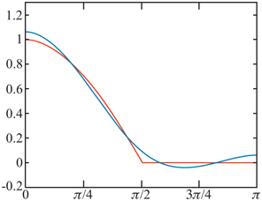
Figure 10.43. The clamped cosine function (in red) versus its nine-coefficient spherical harmonic approximation (in blue). The approximation is quite close. Note the slight dip below and the rise above zero between $π / 2$ and $π$ .

The approximation is remarkably close, although the “wiggling” of the curve between $π / 2$ and $π$ , when it should be zero, is called ringing in signal processing. It typically occurs when a function with high frequencies is approximated with a small number of basis functions, as seen in Section 10.3.2. The clamp to zero at $π / 2$ is a sharp change, which means our clamped cosine function has an infinite frequency signal. Ringing is not noticeable in most cases, but it can be seen under extreme lighting conditions as color shifts or bright “blobs” on the shadowed sides of objects. If the irradiance environment map is used to store only indirect lighting (as often happens), then ringing is unlikely to be a problem. There are prefiltering methods that minimize the issue [1656,1659]. See Figure 10.44.

Figure 10.44. Left: example of visual artifacts caused by ringing. Right: a possible solution is to make the original function smoother, so it can be represented without ringing, a process called “windowing.” (Images courtesy of Peter-Pike Sloan.)

Figure 10.40 shows how an irradiance map derived directly compares to one synthesized by the nine-term function. This SH representation can be evaluated during rendering with the current surface normal $n$ [1458], or can be used to rapidly create a cubic or parabolic map for later use. Such lighting is inexpensive and gives good visual results for the diffuse case.

Dynamically rendered cubic environment maps can be projected onto the SH basis [871,897,1458]. Since cubic environment maps are a discrete representation of the incoming radiance function, the integral over the sphere in Equation 10.21 becomes a sum over the cube map texels:

(10.40)

$\begin{matrix} k_{Lj} = \sum_{t} f_{j} (r [t]) L [t] d ω [t], \end{matrix}$

where t is the index of the current cube map texel, $r [t]$ is the direction vector pointing to the current texel, $f_{j} (r [t])$ is the jth SH basis function evaluated at $r [t]$ , L[t] is the radiance stored in the texel, and $d ω [t]$ is the solid angle subtended by the texel. Kautz [871], King [897], and Sloan [1656] describe how to compute $d ω [t]$ .

To convert the radiance coefficients $k_{Lj}$ into irradiance coefficients, these need to be multiplied by the scaled coefficients of the clamped cosine function $cos {(θ_{i})}^{+}$ :

(10.41)

$\begin{matrix} k_{Ej} = k_{{cos}^{+} j}^{'} k_{Lj} = k_{{cos}^{+} j}^{'} \sum_{t} f_{j} (r [t]) L [t] d ω [t], \end{matrix}$

where $k_{Ej}$ is the jth coefficient of the irradiance function $E (n)$ , $k_{Lj}$ is the jth coefficient of the incoming radiance function $L (l)$ , and $k_{{cos}^{+} j}^{'}$ is the jth coefficient of the clamped cosine function $cos {(θ_{i})}^{+}$ scaled by $\sqrt{4 π / (2 l + 1)}$ (l is the frequency band index).

Given t and the cube map resolution, the factor $k_{{cos}^{+} j}^{'} f_{j} (r [t]) d ω [t]$ is constant for each basis function $f_{j} ()$ . These basis factors can be precomputed offline and stored in cube maps, which should be of the same resolution as the dynamic environment maps that will be rendered. The number of textures used can be reduced by packing a separate basis factor in each color channel. To compute an irradiance coefficient for the dynamic cube map, the texels of the appropriate basis factor map are multiplied with those of the dynamic cube map, and the results are summed. Beyond information on dynamic irradiance cube maps, King [897] provides implementation details on GPU SH projection as well.

Dynamic light sources can be added into an existing SH irradiance environment map. This merge is done by computing the SH coefficients of the lights’ irradiance contributions and adding them to the existing coefficients. Doing so avoids the need to recompute the entire irradiance environment map. It is a straightforward process, since simple analytical expressions exist for the coefficients of point, disk, and spherical lights [583,871,1656,1690]. Summing the coefficients has the same effect as summing the irradiance. Usually these representations are given in zonal harmonics, for a light aligned with the z-axis, and then rotations can be applied to position the light toward an arbitrary direction. Zonal harmonics rotation is a special case of SH rotation (Section 10.3.2) and is much more efficient, requiring only a dot product instead of a full matrix transform. Coefficients for light sources with more complex shapes can be computed by drawing them into an image that is then numerically projected onto the SH basis [1690]. For the special case of a physical sky model, Habel [626] shows a direct expansion of the Preetham skylight in spherical harmonics.

The ease of projection of common analytical light sources into SH is important, as often environment lighting is used to stand in for distant or less-intense light sources. Fill lights are an important case. In rendering, these light source are placed to simulate the indirect light in the scene, i.e., light bouncing off surfaces. Specular contributions are often not computed for fill lights, especially as these lights can be physically large relative to the shaded object and relatively dim compared to other sources of illumination in the scene. These factors make their specular highlights more spread out and less noticeable. This type of light has a real-world analogy in lighting for film and video, where physical fill lights are often used to add lighting in shadows.

In spherical harmonic space it is also simple to do the opposite derivation, that is, to extract analytic light sources from radiance projected in SH. In his survey of SH techniques, Sloan [1656] shows how, given a directional light source with a known axis, it is easy to compute from a SH irradiance representation the intensity that the light should have to minimize the error between itself and the encoded irradiance.

In his previous work [1653] Sloan shows how to select a near-optimal direction by employing only the coefficients in the first (linear) band. The survey also includes a method for extracting multiple directional lights. This work shows that spherical harmonics are a practical basis for light summation. We can project multiple lights into SH and extract a smaller number of directional lights that can closely approximate the projected set. A principled approach to aggregating less important lights is provided by the lightcuts [1832] framework.

Although most commonly used for irradiance, SH projections can be employed to simulate glossy, view-dependent BRDF lighting. Ramamoorthi and Hanrahan [1459] describe one such technique. Instead of a single color, they store in a cube map the coefficients of a spherical harmonic projection encoding the view-dependence of the environment map. However, in practice this technique requires much more space than the prefiltered environment map approaches we have seen earlier. Kautz et al. [869] derive a more economical solution using two-dimensional tables of SH coefficients, but this method is limited to fairly low-frequency lighting.

..................Content has been hidden....................

You can't read the all page of ebook, please click here login for view all page.

Table of Contents for
10 Local Illumination

Chapter 10

Local Illumination

10.1 Area Light Sources

10.1.1. Glossy Materials

10.1.2. General Light Shapes

10.2 Environment Lighting

10.3 Spherical and Hemispherical Functions

10.3.1. Simple Tabulated Forms

10.3.2. Spherical Bases

Spherical Radial Basis Functions

Spherical Gaussians

Spherical Harmonics

Other Spherical Representations

10.3.3. Hemispherical Bases

Ambient/Highlight/Direction

Radiosity Normal Mapping/Half-Life 2 Basis

Hemispherical Harmonics/H-Basis

10.4 Environment Mapping

10.4.1. Latitude-Longitude Mapping

10.4.2. Sphere Mapping

10.4.3. Cube Mapping

10.4.4. Other Projections

10.5 Specular Image-Based Lighting

10.5.1. Prefiltered Environment Mapping

Convolving the Environment Map

10.5.2. Split-Integral Approximation for Microfacet BRDFs

10.5.3. Asymmetric and Anisotropic Lobes

10.6 Irradiance Environment Mapping

10.6.1. Spherical Harmonics Irradiance

Table of Contents for 10 Local Illumination

Create new playlist

Sign In

Sign Up

10.1.1. Glossy Materials

10.1.2. General Light Shapes

10.3.1. Simple Tabulated Forms

10.3.2. Spherical Bases

Spherical Radial Basis Functions

Spherical Gaussians

Spherical Harmonics

Other Spherical Representations

10.3.3. Hemispherical Bases

Ambient/Highlight/Direction

Radiosity Normal Mapping/Half-Life 2 Basis

Hemispherical Harmonics/H-Basis

10.4.1. Latitude-Longitude Mapping

10.4.2. Sphere Mapping

10.4.3. Cube Mapping

10.4.4. Other Projections

10.5.1. Prefiltered Environment Mapping

Convolving the Environment Map

10.5.2. Split-Integral Approximation for Microfacet BRDFs

10.5.3. Asymmetric and Anisotropic Lobes

10.6.1. Spherical Harmonics Irradiance

Table of Contents for
10 Local Illumination