
10
An Efficient Solar Energy Management Using IoT-Enabled Arduino-Based MPPT Techniques
Rita Banik1* and Ankur Biswas2
1 Department of EEE, ICFAI University Tripura, Agartala, Tripura, India
2 Department of CSE, Tripura Institute of Technology, Narsingarh, Tripura, India
Abstract
The amount of irradiance falling on a photovoltaic (PV) system has a significant impact on its performance. To achieve a constant peak power generation in a PV, maximum power point tracking (MPPT) approach is utilized, which employs a control system to enable PV system to run at their highest power output. The study proposes a method to design solar Maximum Power Point (MPP) Tracker based on an improved, fast, and reliable algorithm. The algorithm is inspired by existing Perturb and Observe (P&O) approach for monitoring solar photovoltaic (SPV) maximum power point. The tracker has been created with a low-cost Arduino UNO development kit, powered by an ATmega328P microcontroller that runs at a 16MHz frequency. The model is fast, accurate and utilizes very low power due to its high frequency operations. The circuit was simulated using Proteus and a hardware prototype to realize the operation has also been established. MPPT was responded in a quick and accurate manner to the changes in solar radiation. The algorithm can significantly minimize the power loss as it removes the oscillation around the MPP. The efficiency offered by the tracker is 99.21% under a Standard Test Condition (1000 W/m2 irradiance at 25°C).
Keywords: MPP tracker, perturb and observe, Arduino, microcontroller, SPV
List of Symbols
| MPP | Maximum Power Point |
| PV | Photovoltaic |
| MPPT | Maximum Power Point Tracking |
| P&O | Perturb and Observe |
| Inc. Cond. | Incremental Conductance method |
| PSO | Particle Swarm Optimization |
| PCE | Power Conversion Efficiency |
| ΔP | Change in output power |
| ΔV | Change in output voltage |
| IL | Photo generated current |
| I | Output current |
| ID | Diode current |
| ISH | Shunt resistor current in amperes |
| ref | Photo current at standard reference condition |
| αT | Relative temperature coefficient of the short-circuit current |
| G | Irradiation on the Solar PV module |
| Gref | Reference irradiation (1000 W/m2) |
| Tref | 25°C |
| Isc | Short Circuit Current |
| Voc | Open Circuit Voltage |
10.1 Introduction
Energy sources like coal, oil, and natural gas, are the significant source of energy for the world. But, the combustion of these sources is the primary reason of global warming. Therefore, renewable sources are growing more prevalent amongst two categories of energy viz., conventional and non-conventional, presently. The rising degree of pollutants and dwindling use of traditional energy sources necessitate the utilization of clean and sustainable renewable energy. It is now known that non-renewable resources, such as coal, oil, and others, are nearly on the brink of ending and stocks are expected to be depleted during the next 50 to 120 years. These preceding challenges highlight the need of investigating renewable energy sources that are cleaner, economical, and sustained. Hence, the transition towards solar, wind and hydro is on the rise. Renewable energy sources which include solar, wind, thermal, hydro, biofuel, and tidal power presently meet roughly 20% of world energy requirements. PV electricity powered by solar energy is amongst the most promising renewable energy alternatives since, it requires less money, is simple to install, and is economically feasible. Solar energy are also abundant and the most available than others. Solar energy based renewable sources particularly has garnered a lot of attention which is clean and emission-free because it doesn’t generate harmful pollutants or by-products. As a result, it is a flourishing research industry today that is challenged by new and more effective modes of solar energy use. Solar power conversion into electricity has many areas of use. PV systems are progressively being incorporated into the worldwide electricity grid. The nonlinear structure of PV arrays in terms of ambient circumstances and changeable climatic elements, on contrary, makes it difficult to extract the utmost power produced by the PV modules. Therefore, the PV modules are able to extract a fake MPP and transform less solar energy into electricity. As a result, the efficacy of PV system suffers a decline. The solar cells presently available commercially can only harvest 10–27% of incoming solar radiation [1–7]. Because solar cells have a poor efficiency, it is necessary to guarantee that the maximum amount of solar light reaches the cells. Also, the Variations in sun irradiance and solar heat affect the output of solar cells [8–14]. When it comes to solar plants with a large installed capacity, the efficiency of PV system drops dramatically. As a result, marginally more efficient MPPT techniques can enhance the produced power. Hence, MPPT approaches have been widely explored and developed by researchers. Thus, to obtain a constant production of maximum power in a solar cell, MPPT approach is frequently utilized [15–17]. MPPT is a technology that uses a control system to allow PV systems to run at their highest power productivity. The technology varies in proportion to the number of sensors, it requires, their complexities, costs, converging speed, and precise monitoring under varying irradiance as well as temperature. When the ambient circumstances change and, as a result, the MPP of the module is adjusted, MPPT approaches can help accelerate the computation for a new MPP. Under typical environmental circumstances, an ineffective MPPT approach may, for instance, maintain the MPP with almost no harm to the power delivered to a system. But, if there are numerous moving clouds in short durations or a fake MPP is spotted, this approach may not be able to keep up with the MPP. Unfortunately, this may compromise the PV system’s ability to generate electricity. As a result, selecting the best MPPT approach for the ambient circumstances is critical for maximizing power generation.
Solar cells are integrated with a solar power converter in order to uti-lize MPPT technique to maximize the yield. There are a number of MPPT methods like Parasitic Capacitance, Constant Voltage Method, P&O [18, 19], Inc. Cond., [20, 21]. Nonetheless, everyone has own strengths and drawbacks [22, 23]. The Constant Voltage method is simple but an inefficient method since it collects only 80% of the available maximum. The Open Circuit Voltage method is not an accurate technique and it might not operate at the highest point of power generation exactly. Also, the Short Circuit Current method is not accurate and has low efficiency. The data vary with various weather conditions and locations. The constant value must be chosen carefully, to accurately calibrate the solar panel. The Incremental Conductance (INC) method has higher complexity that reduces the sampling frequency and increases the overall computational time. However, until the MPP is reached, the slope of the PV curve effects the converter duty cycle in fixed or variable step sizes in INC. MPP tracking time is reduced by increasing the step size, however oscillation around MPP still persists [24]. In Parasitic capacitance method, the parasitic capacitance is very small. Hence, when used in larger PV systems, a large capacitor is essential to eliminate the minor ripples in the PV array, potentially lowering the PV array’s parasitic capacitance. In P&O method, the voltage level is observed and perturbed until the maximum power point is grabbed. But since perturbations continually shift direction to maintain the MPP under rapidly changing solar irradiation, steady-state oscillation occurs in P&O, reducing system efficiency and increasing power losses [25]. Fuzzy Logic, Artificial Neural Network, and PSO are other commonly used MPPT techniques. Each of the techniques possesses characteristics with respect to complexity, speed, response and apparatus. A modified P&O technique with improved results by reducing the steady state oscillations was presented by Alik and Jusoh [26]. Tey et al. [27] established evolution algorithm for tracking MPP within few seconds by improving global search space and achieved an accuracy of 99%. Priyadarshi et al. [28] projected an intelligent Fuzzy PSO under unstable atmospheric and load conditions. Execution of an enhanced P&O MPPT technique by Alik and Jusoh [29] offered higher efficiency. In comparison to the standard PSO method, Mao et al. [30] established a PSO-based MPPT algorithm that reduced the steady-state oscillation with an enhanced output. However, because of their ease of use and increased efficiency, P&O and Inc. Cond. are often employed among the many MPPT techniques. However, their implementation suffer difficulty because the changes in incoming sunlight cause movement away from the MPP and the rate of tracking is relatively slower. It is relatively complex and expensive to incorporate other methodologies [31–33]. Most of the techniques suffer from power loss due to oscillation at the MPP. To address the issue, artificial intelligence (AI) methods such as PSO, Bee Colony optimization, GA, and others were created. The difficulty with the AI method is that if the length of the MPP search space is enormous, the timeframe for converging may be too long [34]. Furthermore, if the weather patterns change quickly, the PV system may run at or near the local maximum power points for an extended period of time.
This study presents the implementation of a PV panel controller with a customized MPPT algorithm relied upon P&O method. The method has been improved in that after achieving the MPP, it eliminates the oscillation surrounding the point in order to attain the steady-state. It continuously tracks and records the MPP. The recorded MPP is updated when a difference between ‘power at MPP’ and ‘PV power’ of 5 W is encountered, it is tracked as new MPP (MPPold). When the algorithm achieves a new MPP, it compares it to the old MPP in order to create more power and update the previous MPP. The new MPP values are tested to see if the steady-state has been attained by computing the regular middle point. The new method intends to monitor the maximum power points quickly and efficiently. The slope of the P-V curve is used here to find the maximum power point. To monitor the voltage as well as current change in the PV panel, a DC-DC buck converter is employed. Furthermore, the DC–DC converter selection is crucial since it must monitor the MPP independent of the ambient circumstances. To put it another way, it can’t have a non-operational zone on its I–V characteristic curve to ensure that the greatest amount of energy is transmitted to the load irrespective of the testing conditions. As the buck converter changes the duty cycle, the change in voltage and current of the panel is achieved that leads in a shift in output power (ΔP) in PV panel. The slope  at a particular position of the P-V curve is calculated from ΔP and change in voltage (ΔV). The calculated slope determines the adjustments of the next duty cycle and until the slope reaches zero or near approximate values. The course of tracking shifts in respect to MPP depending on the slope’s side point. The algorithm continually tracks irra-diance changes and rapidly reiterates the computation. The precise nature of the algorithm helps to attain the maximum power point accurately with fewer iterations and sophisticated step size. The Arduino UNO board having ATmega328P processing unit is utilized to execute this computation within milliseconds. The 16MHz on-board clock frequency of Arduino offers this high processing speed with small power consumption that a 5V battery can provide. The following is an outline of the remainder of the paper: Section 10.2 has a concise summary of the impact of irradiance on solar PV efficiency. Section 10.3 describes the design and implementation of the proposed MPP tracker. Section 10.4 discusses the results. Finally, in Section 10.5, the study concludes with a conclusion.
10.2 Impact of Irradiance on PV Efficiency
The performance of PV module is commonly measured using a single operating point under IEC 61215 specified standard test conditions (STC), which includes an irradiance of 1000W/m2, a module temperature of 25°C, and a spectrum of AM1.5. PV system builders can use these ratings to estimate yearly energy yields. Actual PV installation performance, on the other hand, may vary across a wide variety of real-world operating conditions, and a reliable yield estimate should reflect for this. As recommended in the rating methods of the newly formed IEC 61853 series of standards, this can be predicted or determined experimentally. When an ideal current source connected in parallel with an ideal diode, we consider it as an ideal solar cell. In essence, there is no such thing as an ideal solar cell. Hence, the electrical comparable to a non-ideal solar cell, in addition consists of shunt resistance and series resistance component along with a current source and a diode as depicted in Figure 10.1.
Here IL, ID, ISH, and I can be given by,

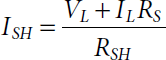

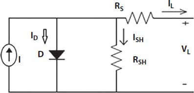
Figure 10.1 A solar cell representation diagram.
So, from the Equation (10.4), it is observed that the solar cell output current (I) is directly dependent on the irradiance (G) which changes the PCE. As a consequence, the solar cell’s output power is changed accordingly which in turn varies the MPP. As a result, an efficient approach is necessary for extracting the MPP to give maximum power through a MPP tracker.
10.2.1 PV Reliability and Irradiance Optimization
10.2.1.1 PV System Level Reliability
Enhancing the efficiency of the module would be only one approach to get more energy out of it. The generated power of the PV at the system level, however, seems to be what matters in the end. So the issue is: what could be done at the system level to boost PV system yields?
Aside from the semiconductors used in PV modules, there are only two components that contribute to a PV system’s efficiency: electrical and mechanical. The former section is in charge of MPP tracking, which is a step in ensuring the function of PV module at MPP on its I-V curve at a certain irradiance and temperature. At PV system’s design stage, this unit cannot be optimized or changed to increase performance but, can be done through MPPT techniques. The other component is the PV system’s mechanical component, which may be tuned by the developer to increase the incident radiance incident on the PV array. Physically adjusting the orientation and tilt angle of the module is the easiest technique to increase solar utility. Hence, there exists a requirement for mechanical monitoring device to follow the sun. Because the most of PV systems are permanently escalated, a single option for alignment and tilting changes based on the geographical location throughout the year.
10.2.1.2 PV Output with Varying Irradiance
The subject of how irradiance affects PV production remains unanswered. In literature, it is learnt how irradiance and temperature impact a PV cell’s production. When all other factors kept invariable, the greater the irradiance, the higher the output current, and hence the higher the power generated. Because the radiation from the sun are the primary source of energy for PV systems, it’s critical that the PV modules are correctly mounted to get the most radiation and minimize partial shading [35]. The unit should point normal to the incoming sun beams in order to collect the greatest irradiation intensity. There exists strong correlation between PV module voltage and current at various solar irradiation levels. One of the finest methods to capture the most solar energy is to use a solar tracking device to trace the sun’s movement in the sky continually. The literature showed how the module generates more current on the vertical axis as the irra-diance increases. Likewise, the voltage and power characteristics of a PV module may be observed at various levels of irradiances. As the irradiance enhances, the module is capable to produce additional power.
10.2.1.3 PV Output with Varying Tilt
The intensity of incoming solar rays on a PV panel determines its optimal performance. As a result, a panel must be angled so that greatest amount of sunrays hit the upper part of the panel vertically. Mounting techniques, terrain topography, and climate conditions all play a role in determining an appropriate tilt [36]. PV modules are typically oriented with the latitudes of the location. Thus, precise orientation is essential for a PV system to achieve full irradiance [37]. The tilt angle and azimuth angle are the two basic angles used to describe array alignment, with the former being the upward angle in between plane and the panel face [38]. Selecting an appropriate tilt angle for a specific installation might help capture the greatest irradiance at a given environmental scenario. Generally, a shorter tilt angle aids productivity in the summer, whereas a greater tilt angle favors low irradiance levels in the winter. Developers should consider the costs of racking and hardware mounting, which may be reduced by lowering the angle of tilt, as well as the potential of wind damage to the array. Solar designers may utilize simple tools created by NREL to discover the ideal tilt and azimuth angles without having to do complex mathematical calculations. There are available tools that lets designers calculate yearly energy output using basic factors to optimize solar utility for a given site.
10.3 Design and Implementation
When numerous units are linked in series, a PV string is generated. In this situation, the string I-V curve is identical to the individual I-V curve of each module, but it is scaled in voltage by the number of modules linked in series, while the current remains constant. PV strings can be as simple as one module or as complex as a series of modules. When strings are coupled in parallel, the current is scaled by the number of threads, but the voltage is equal to the voltage of each individual string. Depending on the size of the system, a PV system might have a single string or numerous strings. Continuing on to the shading impact on PV systems, when one module within a string is shaded, the entire string might lose power due to the limitation of current flowing through the string, similar to the modules level effect. Bypass diodes will clear the shading effect by bypassing the shaded module, as indicated by the modules solution. As a result, the overall string voltage will drop, potentially interfering with the other parallel strings in the system, because the equivalent array voltage is determined by the string with the lowest voltage. As a result, designer opt to include a blocking diode to restrict electricity from travelling back to the weak string, which also eliminates the risk of fire.
The architecture of a solar pv is based on the amount of solar irradiance available at a given location. The input power of daylight or the overall power from radiating sources hitting on a unit area is measured by irradiance. The irradiance obtained by Earth from the sun via the atmosphere is the solar constant for Earth.
Here, Solarex MSX-60 panel is used for simulation through Proteus that provides easy Arduino microcontroller compatibility as shown in Figure 10.2. The detailed specification of the panel is presented in Table 10.1. The I-V and P-V characteristic curves for Solarex MSX-60 are depicted in Figure 10.3. To model the PV panel in Proteus, a controlled current source of 3.8 ampere (A), a diode with modified Spice code, a shunt and series resistance is created. As per the MSX-60 panel specifications, the saturation current Is, ideality factor, number of cells, and band gap energy must be changed in the Spice code. A maximum of 3.8 A and 3.8128 V is generated by each cell at STC i.e. at the temperature (T) 25o C and irradiance (G) 1000 W/m2. Isc of 3.8 A and Voc of 21.1 V is generated by the entire configuration which is encapsulated within a module like structure. The Voltage Controlled Current Source (VCCS) is controlled by DC Voltage Source (DVS) in order to model the Current Source. The diode with spice code is used to control the Saturation current (Is), number of cell, ideality factor [39]. The DVS is coupled to the PV panel as variable load.
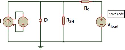
Figure 10.2 The solar panel model under proteus.
Table 10.1 Detailed description of Solarex MSX-60 panel.
| Sl. no. | Features | Rating |
|---|---|---|
| 1 | Power (max) | 60W |
| 2 | Cell type and efficiency | polycrystalline |
| 3 | Voltage at maximum point (Vmp) | 17.1 V |
| 4 | Current at maximum point (Imp) | 3.5A |
| 5 | Open circuit voltage (Voc) | 21.1 V |
| 6 | Short circuit current (Isc) | 3.8 A |
| 7 | Ideality factor | 0.9784 |
| 8 | Shunt Resistance Rsh | 153.5644 Ω |
| 9 | Series Resistance Rs | 0.38572Ω |
| 10 | Test condition: | 1000W/m2, 25°C |

Figure 10.3 The I-V and P-V curves in Solarex MX-60 PV panel.
The typical P&O technique periodically monitors the change in power as the voltage is being perturbed to achieve maximum power from PV arrays. If no change of power occurs, MPP is achieved. The major drawback of the P&O system is the fact that it has a restricted tracking speed because it makes a fixed voltage change in the iterations. It thus oscillates around the MPP area for a while, which leads to poor precision when solar radiation is rapidly changing.
This study presents a novel algorithm as shown in Algorithm 1 that tracks the MPP within less than a second. Here, the P-V curve of the PV array system uses a variable step size to establish the maximum power point. Instead of a fixed duty cycle, the buck converter uses a varied duty cycle in accordance with the slope of the P-V curve. On the right side of MPP, the slope is less than zero while on the left side of MPP the slope is positive, i.e., greater than zero. The step size is therefore regulated automatically that achieves an improvement in tracking speed. Unlike the traditional P&O method, the algorithm after reaching the MPP removes the oscillation surrounding the MPP as it reaches the steady-state [40]. This is achieved in the following way: The algorithm normally tracks the MPP and recorded as ‘Pmpp’ continuously. If (Pmpp – Ppv > ΔP), it is tracked as new MPP (MPPold). There is a variation of 5W (ΔP=5W) in Ppv, if there is a variation of 30 W/m2 in irradiance ‘G’, which represents that G is changed. When the algorithm attains a new MPP, it is compared with MPPold to generate higher power and updates the MPPold. The tracking converges at the boundary (i.e., 0.1-0.9 Voc). The new MPPold is checked as if the steady-state is reached, through computing the regular middle point (Vmid). The voltage is registered as Vmid if the step shifts two successive directions. If the step is Vmid again, the counter is incremented by 1. When the counter hits the limit, the oscillation stops and the step at Vmid also stops. Thus, the oscillation is stopped approximately at the MPP. As a result, the total loss of power is reduced.
10.3.1 The DC to DC Buck Converter
The buck converter is a simple DC-DC converter that outputs a lower voltage than the input voltage. The inductor in a buck converter typically “bucks” or works against the input voltage, thus the name. An ideal buck converter’s output voltage is simply the product of the switching duty cycle and the source voltage. The DC-DC step-down (buck) converter has a controller including one or more inbuilt FETs and an additional inductor, and they provide a good blend of versatility and usability. Buck converters, both synchronous and non-synchronous, simplifies the conceptual design by decreasing the number of external components. Simultaneously, the choices external inductor allows improving the power supply for effi-ciency, size, or price. The DC/DC buck voltage converter and accompanying modeling tools are available to assist almost every need in order to meet the power-supply design issues. The impedance coupled to a PV panel determines its working point. The panel can, therefore, be worked on the maximum power point by adjusting the load impedance. PV panel is a DC source, so the DC-DC converter is applied as shown in the panel to adjust the load impedance. The representation diagram of the DC-DC converter is shown in Figure 10.4. Increasing the duty cycle of the converter will change the impedance. Here, a buck converter is designed for this purpose as per specifications listed in Table 10.2. Through increasing its duty cycle, the converter bucks the Voc of the panel. Thus, Arduino determines the slope of the P-V curve. Arduino from one of its pulse width modulation (PWM) pins fed the successive duty cycle value to the buck converter MOSFET after the required calculations. The impedance, therefore, continues to change and settles at the MPP of the P-V curve. IRFZ44N logic level MOSFET is used that can be directly driven by an Arduino PWM pin.
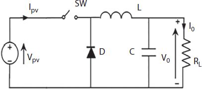
Figure 10.4 Circuit diagram of the designed buck converter.
Table 10.2 Component specifications for the BUCK converter.
| 1. | Inductor | 0.5 mH |
| 2. | Capacitor | 150 µF |
| 3. | Load Resistance | 5 Ω |
| 4. | MOSFET | IRFZ44N Switching Frequency: 50 kHz |
| 5. | Diode | 10BQ040 |
10.3.2 The Arduino Microcontroller
Arduino Uno is an open framework that may be used to create electrical creations. Arduino consists of a hardware configurable programmed circuitry (microcontroller) and software referred as an IDE (Integrated Development Environment), used to create and transfer programming code to the physical board. The Arduino platform has grown in popularity among those who are just getting started with circuits, and for good cause. Unlike many other prior programmable circuitry, the Arduino does not require an additional hardware device (known as a programmer) to transfer new code into the device; instead, a USB cable is all that is required. Furthermore, the Arduino IDE makes programming easier by using a simplified form of C++. Finally, Arduino offers a standard form factor that separates the microcontroller’s tasks into a more manageable packaging. Simply voltage levels are sensed by the Arduino microcontroller. It can accommodate up to 5V of its analog pins. A current sensor is therefore used to capture current values. The sensor is used to sense the panel output current and converts it to a 5 V range in conjunction with a filter circuit. The value would then be transformed to the current equivalent value, which Arduino then uses for calculation. The panel’s output voltage must likewise be scaled down in this range. Hence, a voltage divider circuit has been utilized with a resistance ratio of 1:7 to transform the maximum voltage of 34V within the range of 5V. Since the solar insolation level often changes quickly, the maximum power point is, therefore, to be calculated within a period of time. The schematic diagram is shown in Figure 10.5. Because of its fast processing speed, numerous built-in functionality, acoustic contents (digital operation), and versatility, the Arduino micro-controller board was chosen for this work. The following are some of the other advantages of utilizing Arduino:
- There is no need for external PWM generating equipment.
- It includes a supplementary 5V power supply for the current sensors and LCD operations. Additionally, ATmega328P offers features of high performance, low power consumption, fully static operation, on chip analog comparator and advance RISC architecture. Because of its sophisticated RISC design, the ATmega328P is an 8-bit AVR microcontroller with high efficiency and low power consumption that can execute 131 strong instructions in a single clock cycle. It’s a CPU that’s typically seen in Arduino boards like the Arduino Fio and Arduino Uno. Advantages of ATmega328p are the following:
- Processors are easier to operate since they employ 8bit and 16bit instead of the more difficult 32/64bit.
- With 32k bytes of onboard self-programmable flash program memory and 23 programmable I/O lines, it may be used without any external computational components.
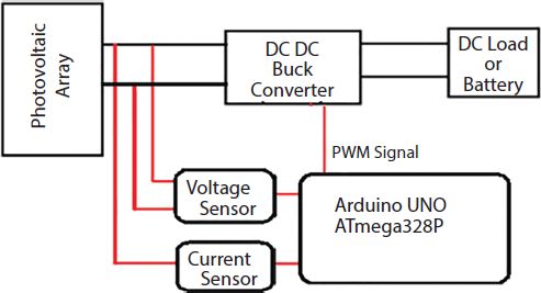
Figure 10.5 The proposed MPP tracker’s schematic design.
Table 10.3 Various features of ATmega328P.
1. Total number of Pins 28 2. Processing Unit RISC 8-Bit AVR 3. Range of operating voltage 1.8 - 5.5 V, 5V as a standard 4. Program Memory and Type 32KB ( Flash) 5. EEPROM 1 KB 6. SRAM 2 KB 7. ADC channels 8 of 10-Bit 8. PWM Pins 6 9. Comparator 1 10. Oscillator up to 20 MHz 11. Timer/counter 3 nos, 8-Bit-2, and 16-Bit-1 - The arithmetic logic unit (ALU) is intrinsically linked to all 31 registers, resulting in a microcontroller that is 10 times quicker than traditional CISC microcontrollers.
- AVR improved RISC instruction set optimized. It’s well-suited for power control, rectifier, and DAC applications owing to the fast PWM mode, which generates high- frequency PWM waveforms.
Other features of ATmega328P are represented in Table 10.3.
10.3.3 Dynamic Response
The response of the developed algorithm is depicted in Figure 10.6 which reveals that the proposed algorithm follows the rapid irradiation changes very quickly. For demonstration, the solar irradiance is changed from 1000 W/m2 to 600 W/m2 from time 2 sec and kept up to 4 sec. Again the irradiance is raised to 1000 W/m2 at time 4 sec. The corresponding voltage and power are also shown. In both cases, the time required to track the MPP is 0.2 seconds. It is shown that, for a given change in solar irradiation, the PV power changes proportionally.

Figure 10.6 The PV power and voltage under varying solar irradiance.
10.4 Result and Discussions
In this study, Proteus is used for simulation. To simulate the PV module in Proteus, the analogous circuit is created using a controlled current source and a diode using customized Spice code, which is then used to develop a true PV panel model. The setting of the PV panel is as follows: Voc = 21.1V, Isc = 3.8A, and under STC, the maximum output power of PV is 60W. Global irradiance is varied as 1000 W/m2, 811 W/m2, 676 W/m2, 540 W/m2, 405 W/m2, and 270 W/m2. In PV systems, the matter of concern is the overall current and voltage that the PV module can produce, hence we create the Module I-V curve, also known as the current-voltage curve. The curve depicts the voltage and current under various operating circumstances. For instance, the maximum current refers to the short- circuit condition (when the positive and negative connectors of the PV module are attached without load, allowing extremely greater current to flow), whereas the maximum voltage arises when the positive and negative connectors of the PV module are attached to any load, allowing no power to flow. When the current and voltage beginning at the open-circuit situation is examined (where the voltage is greatest and the current is zero), and increasing the load of the circuit, the current begins to climb as the voltage declines until it approaches zero at the short-circuit condition (where the current is maximum). Other approach to see the I-V curve is to transform it to a power-voltage relationship. In this scenario, we may refer to it as the PV module’s (P-V) curve. Like an I-V curve, the maximum voltage appears when the circuit is open and the current is zero, and the lowest voltage occurs when the circuit is closed and the current is largest. Because power can considered as voltage times current (P=VXI), power is exactly zero among both short-circuit and open-circuit states because either voltage or current is zero at any of these sites. If we watch the power and voltage beginning at the open-circuit state (where the voltage is greatest and the power is zero), then increasing the load of the circuit, the power begins to climb and the voltage lowers until it reaches the value at MPP (where power is maximum and voltage is zero). As the load is raised further, the voltage continues to decline. Yet, the power would decline until it hits zero in a short-circuit circumstance (where the both voltage and power are zero). It is revealed that the peak power on the P-V curve is much easier to identify than on the I-V curve since it represents a hump. The MPP has been effectively tracked and the maximum power obtained as 58.59 W. The current and voltage were measured as 3.12 A and 18.78 V respectively. The model has been checked in order to confirm if the MPP can be monitored each time. The model effectively and reliably recorded MPPs at each point which is illustrated in Figure 10.7. At lower irradiance levels the power attained was lower. For example, at 811 W/m2, 676 W/m2, 540 W/m2, 405 W/m2, and 270 W/m2 the power attained is 51.97 W, 47.49 W, 36.21 W, 27.92 W and 17.88 W, respectively. It also validates the predicted behavior of a solar-energy-converting device: output power decreases as irradiation decreases. The impact of increasing panel temperature on reduced power is not immediately apparent, but it is consistent with a large influence on open-circuit voltage Voc. An external 60 W solar panel was attached to the tracker. Table 10.4 illustrates the Vmp, Imp, Pmp, and efficiency of the tracker for various levels of irradiance. The efficiency of the tracker was measured within the range of 94.48% to 99.21%. The proposed method is compared to various MPPT techniques [41] as demonstrated in Table 10.5.
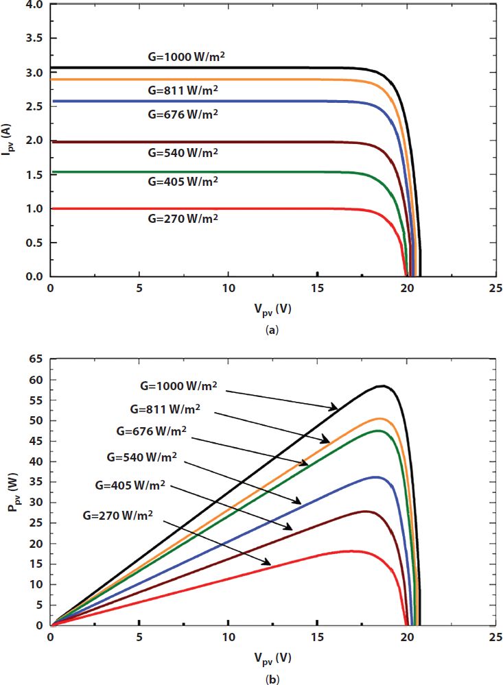
Figure 10.7 Output characteristics curve while tracking the MPP at different irradiance for Solarex MSX-60 (a) I-V (b) P-V characteristics.
Table 10.4 Comparison of simulated MPPs with measured power and efficiencies at various irradiances.

Table 10.5 An assessment of the proposed method to various MPPT techniques.
| Methods | Cost | Time to track MPP in seconds | Efficiency % |
|---|---|---|---|
| Constant Voltage | - | 0.2-0.4 | 95.16 |
| Fixed duty cycle | - | - | 57.80 |
| Incremental Conductance | Costly | 0.5 | 98.53 |
| Existing P&O | - | 0.2-0.4 | 98.40 |
| Neural network based P&O [42] | - | 0.2-0.5 | 94-98 |
| Improved INC [43] | Cost-effective | 0.33 | 98.91 |
| Proteus-Based Arduino Board Environments [44] | - | 0.2-0.96 | 99.4 |
| Improved INC [45] | - | 0.35-0.39 | 94.83 |
| Modified P&O (Proposed) | Cost-effective | 0.2 | 99.21 |
The proposed tracker is considered to be cost effective since it uses low cost sensors on Arduino board to track the irradiances. The time required to track the MPP is 0.2 seconds which is considerably very low. Finally, the efficiency of the tracker was measured within the range of 94.48% to 99.21%, which is quite satisfactory.
10.5 Conclusions
PV energy production has recently emerged as a potential source of energy because to its several advantages, including cheap maintenance costs, no need for relocation, and also no pollutants. Yet, the poor effi-cacy of panels and the expensive cost of PV system deployment may be deterrents to its adoption. Furthermore, the nonlinear behavior and strong reliance of PV modules on solar irradiance and temperature provide significant hurdles in PV system researches. To circumvent these constraints, the functioning of the PV system just at MPP is a necessity that can increase the PV reliability and capacity. As a result, the MPPT algorithm is applied. This paper showed a new approach to quickly and accurately track the MPP of solar panels. A high-speed processor clocked microcontroller board (Arduino UNO) was used to design the tracker. Proteus software is utilized to design and simulate the model. As Arduino could not accept voltages greater than 5 V, a voltage sensor is utilized to lower the Voltage level to some other value between (Vd) [0, 5] that could be recognized by Arduino. The current sensor is utilized to convey a representation of the PV panel power to the Arduino. A modified P&O algorithm is established with zero oscillation at the MPP. The new method was written in the Arduino programming language before being loaded into the microcontroller. The circuitry functioned autonomously in according to the algorithm and allowed for real-time decision making. The built MPP tracker has also been evaluated in an outside location using the experimental configuration. The circuit produces output based on the findings of the simulated model. The model was calculated as 99.21 percent as maximum efficiency. The new technique may be considered as addressing the drawbacks of traditional P&O and improving the overall efficiency.
References
- 1. Banakhr, F.A. and Mosaad, M.I., High performance adaptive maximum power point tracking technique for off-grid photovoltaic systems. Sci. Rep., 11, 20400, 2021, doi: https://doi.org/10.1038/s41598‐021‐99949‐8.
- 2. Kermadi, M., Salam, Z., Eltamaly, A.M., Ahmed, J., Mekhilef, S., Larbes, C., Berkouk, E., Recent developments of MPPT techniques for PV systems under partial shading conditions: A critical review and performance evaluation. IET Renew. Power Gener., 14, 3401–3417, 2020.
- 3. Al-Majidi, S., Abbod, M.F., Al-Raweshidy, H.S., A novel maximum power point tracking technique based on fuzzy logic for photovoltaic systems. Int. J. Hydrog. Energy, 43, 14158–14171, 2018.
- 4. Salman, S., Xin, A.I., Zhouyang, W.U., Design of a P&-O algorithm based MPPT charge controller for a stand-alone 200W PV system. Prot. Control Mod. Power Syst., 3, 25, 2018, doi: https://doi.org/10.1186/s41601‐018‐0099‐8.
- 5. Sarika, P.E., Jacob, J., Mohammed, S., Paul, S., A novel hybrid maximum power point tracking technique with zero oscillation based on P&O algorithm. Int. J. Renew. Energy Res., 10, 1962–1973, 2020.
- 6. Başoğlu, M.E. and Çakır, B., Comparisons of MPPT performances of isolated and non-isolated DC–DC converters by using a new approach. Renew. Sust. Energ. Rev., 60, 1100–1113, 2016.
- 7. Killi, M. and Samanta, S., An adaptive voltage-sensor-based MPPT for photovoltaic systems with SEPIC converter including steady-state and drift analysis. IEEE Trans. Ind. Electron., 62, 12, 2015.
- 8. Thongsuwan, W., Sroila, W., Kumpika, T. et al., Antireflective, photocata-lytic, and superhydrophilic coating prepared by facile sparking process for photovoltaic panels. Sci. Rep., 12, 1675, 2022, doi: https://doi.org/10.1038/s41598‐022‐05733‐7.
- 9. Dhimish, M. and Tyrrell, A.M., Power loss and hotspot analysis for photovoltaic modules affected by potential induced degradation. NPJ Mater. Degrad., 6, 11, 2022, doi: https://doi.org/10.1038/s41529‐022‐00221‐9.
- 10. Grubisic-Cabo, F., Nizetic, S., Marco, T.G., Photovoltaic panels: A review of the cooling technique. Trans. Famena, 40, SI-1, 63–74, 2016.
- 11. Ramaprabha, R. and Mathur, B.L., Impact of partial shading on solar PV module containing series connected cells. Int. J. Recent Trends Eng., 2, 7, 56–60, 2009.
- 12. Moharram, K.A., Abd-Elhady, M.S., Kandil, H.A., El-Sherif, H., Enhancing the performance of photovoltaic panels by water cooling. Ain Shams. Eng. J., 4, 4, 869–877, 2013.
- 13. Alonso-Garcia, M.C., Ruiz, J.M., Chenlo, F., Experimental study of mismatch and shading effects in the I–V characteristic of a photovoltaic module. Sol. Energy Mater. Sol. Cells, 90, 3, 329–340, 2006.
- 14. Kawamura, H., Naka, K., Yonekura, N., Yamanaka, S., Kawamura, H., Ohno, H., Naito, K., Simulation of I–V characteristics of a PV module with shaded PV cells. Sol. Energy Mater. Sol. Cells, 75, 3, 613–621, 2003.
- 15. Danandeh, M.A. and Mousavi, S.M.G., Comparative and comprehensive review of maximum power point tracking methods for PV cells. Renew. Sustain. Energy Rev., 82, 2743–2767, 2018.
- 16. Dandoussou, A., Kamta, M., Bitjoka, L., Wira, P., Kuitché, A., Comparative study of the reliability of MPPT algorithms for the crystalline silicon photovoltaic modules in variable weather conditions. J. Electr. Syst. Inf. Technol., 4, 1, 213–224, 2017.
- 17. Pant, S. and Saini, R.P., Comparative study of MPPT techniques for solar photovoltaic system. International Conference on Electrical, Electronics and Computer Engineering (UPCON), pp. 1–6, 2019, doi: 10.1109/ UPCON47278.2019.8980004.
- 18. Salman, S., AI, X., WU, Z., Design of a P-&-O algorithm based MPPT charge controller for a stand-alone 200W PV system. Prot. Control Mod. Power Syst., 3, 25, 2018, doi: https://doi.org/10.1186/s41601‐018‐0099‐8.
- 19. Elgendy, M.A., Zahawi, B., Atkinson, D.J., Assessment of perturb and observe MPPT algorithm implementation techniques for PV pumping applications. IEEE Trans. Sustain. Energ., 3, 1, 21–33, 2012.
- 20. Shang, L., Guo, H., Zhu, W., An improved MPPT control strategy based on incremental conductance algorithm. Prot. Control Mod. Power Syst., 5, 14, 2020.
- 21. Tey, K.S., Mekhilef, S., Seyedmahmoudian, M., Horan, B., Oo, A.M., Stojcevski, A., Improved differential evolution-based MPPT algorithm using SEPIC for PV systems under partial shading conditions and load variation. IEEE Trans. Ind. Inform.,14, 10, 4322–4333, 2018, doi: https://doi.org/10.1109/TII.2018.2793210.
- 22. Hlaili, M. and Hfaiedh, M., Comparison of different MPPT algorithms with a proposed one using a power estimator for grid connected PV systems. Int. J. Photoenergy, 2016, Article ID 1728398, pages 10, 2016. 10.1155/2016/1728398.
- 23. Carannante, G., Fraddanno, C., Pagano, M., Piegari, L., Experimental performance of MPPT algorithm for photovoltaic sources subject to inhomogeneous insulation. IEEE Trans. Ind. Electron., 56, 11, 4374–4380, 2009.
- 24. Kumar, N., Hussain, I., Singh, B., Panigrahi, B.K., Self-adaptive incremental conductance algorithm for swift and ripple-free maximum power harvesting from PV array. IEEE Trans. Ind. Informat., 14, 5, 2031–2041, 2018.
- 25. Jiang, L.L., Srivatsan, R., Maskell, D.L., Computational intelligence techniques for maximum power point tracking in PV systems: A review. Renew. Sustain. Energy Rev., 85, 14–45, 2018.
- 26. Alik, R. and Jusoh, A., Modified Perturb and Observe (P&O) with checking algorithm under various solar irradiation. Sol. Energy, 148, 128–139, 2017, doi: https://doi.org/10.1016/j.solener.2017.03.064.
- 27. Tey, K.S. and Mekhilef, S., Modified incremental conductance MPPT algorithm to mitigate inaccurate responses under fast-changing solar irradiation level. J. Sol. Energy, 101, 333–342, 2014.
- 28. Priyadarshi, N., Padmanaban, S., Kiran, M.P., Sharma, A., An extensive practical investigation of FPSO-based MPPT for grid integrated PV system under variable operating conditions with anti-islanding protection. IEEE Syst. J., 13, 2, 1861–1871, 2018, doi: https://doi.org/10.1109/JSYST.2018.2817584.
- 29. Alik, R. and Jusoh, A., An enhanced P&O checking algorithm MPPT for high tracking efficiency of partially shaded PV module. Sol. Energy, 163, 570–580, 2018, doi: https://doi.org/10.1016/J.SOLENER.2017.12.050.
- 30. Rizzo, S.A. and Scelba, G., ANN based MPPT method for rapidly variable shading conditions. Appl. Energy, 145, 124–132, 2015.
- 31. Mao, M., Zhang, L., Duan, Q., Oghorada, O., Duan, P., Hu, B., A Two-stage particle swarm optimization algorithm for MPPT of partially shaded PV arrays. Int. J. Green Energy, 14, 694–702, 2017, doi: https://doi.org/10.1080/15435075.2017.1324792.
- 32. Kulaksız, A.A. and Akkaya, R., A genetic algorithm optimized ANN-based MPPT algorithm for a stand-alone PV system with induction motor drive. Sol. Energy, 86, 9, 2366–2375, 2012.
- 33. Larbes, C., Cheikh, S.A., Obeidi, T., Zerguerras, A., Genetic algorithms opti-mized fuzzy logic control for the maximum power point tracking in photovoltaic system. Renew. Energy, 34, 10, 2093–2100, 2009.
- 34. Hua, C.-C. and Zhan, Y.-J., A hybrid maximum power point tracking method without oscillations in steady-state for photovoltaic energy systems. Energies, 14, 5590, 2021, doi: https://doi.org/10.3390/en14185590.
- 35. Babatunde, A., Abbasoglu, S., Senol, M., Analysis of the impact of dust, tilt angle and orientation on performance of PV Plants. Renew. Sust. Energ. Rev., 90, 1017–1026, 2018.
- 36. Almeida, M.A.P., Recent advances in solar cells, in: Solar Cells, Sharma, S., Ali, K. (eds),. Springer, Cham., 2020. https://doi.org/10.1007/978‐3‐030‐36354‐3_4
- 37. Babatunde, A.A. and Abbasoglu, S., Evaluation of field data and simulation results of a photovoltaic system in countries with high solar radiation. Turk. J. Elec. Eng. Comp. Sci., 23, 1608–1618, 2015.
- 38. Motahhir, S., Chalh, A., Ghzizal, A., Sebti, S., Derouich, A., Modeling of photovoltaic panel by using proteus. J. Eng. Sci. Technol. Rev., 10, 2, 8– 13, 2017.
- 39. Hua, C.-C. and Chen, Y.-M., Modified perturb and observe MPPT with zero oscillation in steady-state for PV systems under partial shaded conditions, in: 2017 IEEE Conference on Energy Conversion (CENCON), pp. 5–9, 2017, DOI: 10.1109/CENCON.2017.8262448.
- 40. Hafez, A., Soliman, A., El-Metwally, K., Ismail, I., Tilt and azimuth angles in solar energy applications–A review. Renew. Sust. Energ. Rev., 15, 713–720, 2011.
- 41. Tofoli, F.L., Pereira, D., Paula, W.J., Comparative study of maximum power point tracking techniques for photovoltaic systems. Int. J. Photoenergy, 2015, Article ID 812582, 10 pages, 2015, doi: http://dx.doi.org/10.1155/2015/812582.
- 42. Kacimi, N., Grouni, S., Idir, A., Boucherit, M.S., New improved hybrid MPPT based on neural network-model predictive control-kalman filter for photovoltaic system. Indones. J. Electr. Eng. Comput. Sci., 20, 3, 1230, 2020.
- 43. Xu, L., Cheng, R., Yang, J., A new MPPT technique for fast and efficient tracking under fast varying solar irradiation and load resistance. Int. J. Photoenegry, Article ID 6535372, 18 pages, 2020.
- 44. Chellakhi, A., Beid, S.E., Abouelmahjoub, Y., Implementation of a novel MPPT tactic for PV system applications on MATLAB/Simulink and proteus- based Arduino Board Environments. Int. J. Photoenergy, Article ID 6657627, 19 pages, 2021, doi: https://doi.org/10.1155/2021/6657627.
- 45. El Hassouni, B., Armani, A.G., Haddi, A., A new MPPT technique for optimal and efficient monitoring in case of environmental or load conditions variation. Int. J. Inf. Tec. App. Sci., 3, 2, 18–28, 2021, doi: https://doi.org/10.52502/ijitas.v3i2.16.
Note
- *Corresponding author: [email protected]