
Chapter 4
Learning with K-Nearest Neighbors
IN THIS CHAPTER
![]() Understanding K-Nearest Neighbors in a basic way
Understanding K-Nearest Neighbors in a basic way
![]() Working with the right k parameter
Working with the right k parameter
![]() Using KNN to perform regression
Using KNN to perform regression
![]() Using KNN to perform classification
Using KNN to perform classification
Previous chapters in this minibook demonstrate that you have multiple options when it comes to performing regression and classification tasks. The K-Nearest Neighbors (KNN) algorithm is another way to perform these tasks (along with others) and it has its own sets of pros and cons. The chapter begins by introducing you to KNN and showing you some of the more basic tasks you can perform with it. Along the way, you discover how KNN differs from other methods of performing both regression and classification.
The next part of the chapter discusses tuning. The k parameter provides the means to tune your algorithm. The need for tuning is high with KNN because of the way it works. This part of the chapter helps you understand, through demonstration, why the k parameter is so important and how to choose one correctly.
The final sections of this chapter look at regression and classification. You use regression to predict future values and classification to determine the type of something. Both tasks are essential in machine learning and deep learning. However, you can employ regression and classification in a substantial number of other ways.
 You don’t have to type the source code for this chapter manually. In fact, using the downloadable source is a lot easier. The source code for this chapter appears in the
 DSPD_0304_KNN.ipynb source code file for Python and the DSPD_R_0304_KNN.ipynb source code file for R. See the Introduction for details on how to find these source files.
Considering the History of K-Nearest Neighbors
Some confusion surrounds the history of KNN, partly because it's the work of so many people. In many cases, articles ascribe the initial idea to Evelyn Fix and J. L. Hodges, as described in an unpublished U.S. Air Force School of Aviation Medicine report in 1951 (http://www.scholarpedia.org/article/K-nearest_neighbor).
The paper must have gotten lost, because it wasn’t until 1967 that Thomas M. Cover and Peter E. Hart worked out some of the formal KNN properties. The history of KNN shows that the methodology relies on incremental innovations:
- 1970: M. E. Hellman added new rejection approaches.
- 1975: Keinosuke Fukunaga and Larry D. Hostetler refined density estimates (with respect to the Bayes error rate).
- 1976: Sahibsingh A. Dudani introduced a distance-weighted KNN rule (WKNN).
- 1978: T. Bailey and A. K. Jain reexamined the relationship between unweighted KNN and WKNN, showing that WKNN can achieve a lower error rate in some cases.
- 1983: A. Jozwik developed a fuzzy KNN classification method.
- 1985: James M. Keller, Michael R. Gray, and James A. Givens presented three methods for using the fuzzy KNN classification method.
- 2000: Sergio Bermejo and Joan Cabestany presented adaptive soft learning KNN classifiers.
Probably a great many other people have contributed to KNN, so it’s hard to say that KNN as it appears today is the result of any one person’s work. However, the idea for KNN didn’t come out of the blue, nor was it some late-night inspiration. Some references say that KNN has much older sources (see http://37steps.com/4370/nn-rule-invention/ for details).
One of these inspirational sources is Occam's razor (http://math.ucr.edu/home/baez/physics/General/occam.html), which essentially says that the hypothesis with the fewest assumptions is probably the correct one. You can actually find this rule stated in so many ways that it boggles the mind, but the basic idea is always the same: Simple is better.
Even though Occam performed his work in the fourteenth century, some sources assert that Occam’s work relied heavily on the still older work of Ibn al-Haytham (965 to 1040) (http://www.ibnalhaytham.com/). This scientist used a precursor of the modern scientific method to explain many things about how the eye acts as a light sensor, and he demonstrated that the brain actually sees the light. In short, KNN is one of the few algorithms that you really can’t pin down as having been invented at any particular time. As with many good scientific methods, it has been in development for a long time.
Learning Lazily with K-Nearest Neighbors
This section talks about the basics of KNN: how and why they work. You begin by considering the basis of KNN and work through several examples in the sections that follow.
Understanding the basis of KNN
KNN isn’t about building rules from data based on coefficients or probability. Rather, KNN works on the basis of similarities. When you have to predict something like a class, you may do best by finding the most similar observations to the one you want to classify or estimate. You can then derive the answer you need from the similar cases.
Observing how many observations are similar doesn’t imply learning something, but rather measuring. Because KNN isn’t learning anything, it’s considered lazy, and you’ll hear it referenced as a lazy learner or an instance-based learner. The idea is that similar premises usually provide similar results, and you don’t want to forget to get such low-hanging fruit before trying to climb the tree!
The algorithm is fast during training because it only has to memorize data about the observations. It actually calculates more during predictions. When it encounters too many observations, the algorithm can become slow and memory consuming. You’re best advised not to use it with big data, or predicting anything may take almost forever! Moreover, this simple and effective algorithm works better when you have distinct data groups without too many variables involved because the algorithm is also sensitive to the dimensionality curse.
The curse of dimensionality happens as the number of variables increases. Consider a situation in which you’re measuring the distance between observations and, as the space becomes larger and larger, it becomes difficult to find real neighbors — a problem for KNN, which sometimes mistakes a far observation for a near one. Rendering the idea is just like playing chess on a multidimensional chessboard. When playing on the classic 2-D board, most pieces are near, and you can more easily spot opportunities and menaces for your pawns when you have 32 pieces and 64 positions. However, when you start playing on a 3-D board, such as those found in some sci-fi films, your 32 pieces can become lost in 512 possible positions. Now just imagine playing with a 12-D chessboard. You can easily misunderstand what is near and what is far, which is what happens with KNN.
 You can still make KNN smart in detecting similarities between observations by removing redundant information and simplifying the data dimensionality using data-reduction techniques.
Predicting after observing neighbors
For an example showing how to use KNN, you can start with the following digits dataset, also used in the “Considering when classes are more” section of Book 3, Chapter 2, which relies on logistic regression to perform classification. KNN is particularly useful, just like Naïve Bayes, when you have to predict many classes, or in situations that require you to build too many models or rely on a complex model.
from sklearn.datasets import load_digits
from sklearn.decomposition import PCA
digits = load_digits()
train = range(0, 1700)
test = range(1700, len(digits.data))
pca = PCA(n_components = 25)
pca.fit(digits.data[train])
X = pca.transform(digits.data[train])
y = digits.target[train]
tX = pca.transform(digits.data[test])
ty = digits.target[test]
The KNN algorithm is quite sensitive to outliers. Moreover, you have to rescale your variables and remove some redundant information. In this example, you use Principle Component Analysis (PCA) (see https://towardsdatascience.com/a-one-stop-shop-for-principal-component-analysis-5582fb7e0a9c for a discussion of PCA when used alone) to perform the analysis.
Rescaling is not necessary because the data represents pixels, which means that it’s already scaled. You can avoid the problem with outliers by keeping the neighborhood small, that is, by not looking too far for similar examples.
Knowing the data type can save you a lot of time and many mistakes. For example, in this case, you know that the data represents pixel values. Doing Exploratory Data Analysis (EDA) (as described in the “Understanding variable transformations” section of Book 3, Chapter 1) is always the first step and can provide you with useful insights, but getting additional information about how the data was obtained and what the data represents is also a good practice and can be just as useful. To see this task in action, you reserve cases in tX and try a few cases that KNN won't look up when looking for neighbors:
from sklearn.neighbors import KNeighborsClassifier
kNN = KNeighborsClassifier(n_neighbors=5, p=2,
metric='euclidean')
kNN.fit(X, y)
The output shows the actual classifier configuration:
KNeighborsClassifier(algorithm='auto', leaf_size=30,
metric='euclidean', metric_params=None,
n_jobs=None, n_neighbors=5, p=2,
weights='uniform')
KNN uses a distance measure to determine which observations to consider as possible neighbors for the target case. The discussion of the DistanceMetric class at https://scikit-learn.org/stable/modules/generated/sklearn.neighbors.DistanceMetric.html tells about the available options. You can easily change the predefined distance using the p parameter:
-
When
pis 2, use the Euclidean distance, which is the distance between two points on a plane (a concept that you likely studied at school). In a K-means application, each data point is a vector of features, so when comparing the distance of two points, you do the following:- Create a list containing the differences of the elements in the two vectors.
- Square all the elements of the difference vector.
- Calculate the square root of the summed elements.
In the end, the Euclidean distance is really just a big sum. When the variables making up the difference vector are significantly different in scale from each other, you end up with a distance dominated by the elements with the largest scale. Rescaling the variables is important so that they use a similar scale before applying the K-means algorithm. You can use a fixed range or a statistical normalization with zero mean and unit variance to achieve this goal.
- When
pis 1, use the Manhattan distance metric, which is the absolute distance between observations. In a 2-D square, when you go from one corner to the opposite one, the Manhattan distance is the same as walking the perimeter, whereas Euclidean is like walking on the diagonal. Although the Manhattan distance isn't the shortest route, it’s a more realistic measure than Euclidean distance, and it’s less sensitive to noise and high dimensionality.
Usually, the Euclidean distance is the right measure, even though the KNeighborsClassifier default is the Minkowski distance (https://people.revoledu.com/kardi/tutorial/Similarity/MinkowskiDistance.html). Sometimes the Euclidean distance can give you worse results, especially when the analysis involves many correlated variables. The following code shows that the analysis seems fine using the Euclidean distance in this case:
print('Accuracy: %.3f' % kNN.score(tX,ty) )
print('Prediction: %s Actual: %s'
% (kNN.predict(tX[-15:,:]),ty[-15:]))
The code returns the accuracy of 99 percent for this example and a sample of the predictions you can compare with the actual values in order to spot differences:
Accuracy: 0.990
Prediction: [2 2 5 7 9 5 4 8 1 4 9 0 8 9 8]
Actual: [2 2 5 7 9 5 4 8 8 4 9 0 8 9 8]
Even though this example does well with the Euclidean distance, you may need to try other distance measures to get accurate results with your data. Verifying the results is always the best idea.
Choosing the k parameter wisely
A critical parameter that you have to define in KNN is k. As k increases, KNN considers more points for its predictions, and the decisions are less influenced by noisy instances that could exercise an undue influence. Your decisions are based on an average of more observations, and they become more solid. When the k value you use is too large, you start considering neighbors that are too far, sharing less and less with the case you have to predict.
It’s an important trade-off. When the value of k is less, you consider a more homogeneous pool of neighbors but can more easily make an error by taking the few similar cases for granted. When the value of k is more, you consider more cases at a higher risk of observing neighbors that are too far or that are outliers. Getting back to the previous example with handwritten digit data, you can experiment with changing the k value, as shown in the following code:
for k in [1, 5, 10, 50, 100, 200]:
kNN = KNeighborsClassifier(n_neighbors=k, p=2,
metric='euclidean')
kNN.fit(X, y)
print('for k = %3i accuracy is %.3f'
% (k, kNN.score(tX, ty))
After running this code, you get an overview of what happens when k changes and determine the value of k that best fits the data:
for k = 1 accuracy is 0.979
for k = 5 accuracy is 0.990
for k = 10 accuracy is 0.969
for k = 50 accuracy is 0.959
for k = 100 accuracy is 0.959
for k = 200 accuracy is 0.907
Through experimentation, you find that setting n_neighbors (the parameter representing k) to 5 is the optimum choice, resulting in the highest accuracy. Using just the nearest neighbor (n_neighbors =1) isn't a bad choice, but setting the value above 5 instead brings decreasing results in the classification task.
As a rule of thumb, when your dataset doesn’t have many observations, set k as a number near the squared number of available observations. However, no general rule exists, and trying different k values is always a good way to optimize your KNN performance. Always start from low values and work toward higher values.
Leveraging the Correct k Parameter
The k parameter is the one you can work on tuning to make a KNN algorithm perform well in prediction and regression. The following sections describe how to use the k parameter to tune the KNN algorithm.
Understanding the k parameter
The k value, an integer number, is the number of neighbors that the algorithm has to consider in order to figure out an answer. The smaller the k parameter, the more the algorithm will adapt to the data you are presenting, risking overfitting but nicely fitting complex separating boundaries between classes. The larger the k parameter, the more it abstracts from the ups and downs of real data, which derives nicely smoothed curves between classes in data but does so at the expense of accounting for irrelevant examples.
As a rule of thumb, first try the nearest integer of the square root of the number of examples available as a k parameter in KNN. For instance, if you have 1,000 examples, start with k = 31 (or k = 32 because the actual square root is 31.62277660168379) and then decrease the value in a grid search backed up by cross-validation.
Using irrelevant or unsuitable examples is a risk that a KNN algorithm takes as the number of examples it uses for its distance function increases. The previous illustration of the problem of data dimensions shows how to compute a well-ordered data space as a library in which you could look for similar books in the same bookshelf, bookcase, and section. However, things won’t look so easy when the library has more than one floor. At that point, books upstairs and downstairs are not necessarily similar, therefore being near but on a different floor won’t assure that the books are similar. Adding more dimensions weakens the role of useful ones, but that is just the beginning of your trouble.
Now imagine having more than the three dimensions in daily life (four if you consider time). The more dimensions, the more space you gain in your library. (As in geometry, you multiply dimensions to get an idea of the volume.) At a certain point, you will have so much space that your books will fit easily with space left over. For instance, you could have 20 binary variables, with each representing a dimension — but think of the dimensions as providing separation, as with a category. Books on space-based science fiction that include dolphins could appear on one bookshelf, in a particular bookcase, in a particular section, on a particular floor, at a particular time (and so on, until you come up with 20 levels of separation). You could have 2 raised to the 20th power combinations; that is, 1,048,576 possible different dimensions — places to put books. It’s great to have a million book locations, but if you don’t have a million books to fill them (so there is at least one book in each location), most of your library will be empty. So you obtain a book and then look for similar books to place in the same bookcase (those that fulfill all the requirements for all 20 dimensions). The chances of finding two books that are so alike that they meet the same precise values for 20 dimensions are slim, so you end up putting the next book in an empty location, but still, your library is relatively empty. Think about it: You start with The Hitchhiker's Guide to the Galaxy and end up having a book on gardening as its nearest neighbor. This is the curse of dimensionality. The more dimensions, the more likely you are to experience some false similarity, misunderstanding far for near.
Using the right-sized k parameters alleviates the problem because the more neighbors you have to find, the further KNN has to look — but you have other remedies. PCA can compress the space, making it denser and removing noise and irrelevant, redundant information. In addition, feature selection can do the trick, selecting only the features that can really help KNN find the right neighbors.
KNN is an algorithm that’s sensitive to outliers. Neighbors on the boundaries of your data cloud in the data space could be outlying examples, causing your predictions to become erratic. You need to clean your data before using it. Running a K-means first can help you identify outliers gathered into groups of their own. (Outliers love to stay in separate groups; you can view them as the hermit types in your data.) Also, keeping your neighborhood large can help you minimize (but sometimes not avoid completely) the problem at the expense of a lower fit to the data (more bias than overfitting).
Experimenting with a flexible algorithm
The KNN algorithm has slightly different implementations in R and Python. In R, the algorithm is found in the library named class. The function is just for classification and uses only the Euclidean distance for locating neighbors. It does offer a convenient version with automatic cross-validation for discovering the best k value. There’s also another R library, FNN (https://cran.r-project.org/web/packages/FNN/index.html), which contains one KNN variant for classification and another for regression problems. The peculiarity of the FFN functions is that they can deal with the complexity of distance computations using different algorithms, but the Euclidean distance is the only distance available. (See the R downloadable source for additional details.)
The Python experiment with KNN uses the Python class from Scikit-learn and demonstrates how such a simple algorithm is quite adept at learning shapes and nonlinear arrangements of examples in the data space. The block of code prepares a tricky dataset: In two dimensions, two classes are arranged in bull’s-eye concentric circles, as shown in Figure 4-1.
import numpy as np
from sklearn.datasets import make_circles, make_blobs
strange_data = make_circles(n_samples=500, shuffle=True,
noise=0.15, random_state=101,
factor=0.5)
center = make_blobs(n_samples=100, n_features=2,
centers=1, cluster_std=0.1,
center_box=(0, 0))
first_half = np.row_stack((strange_data[0][:250,:],
center[0][:50,:]))
first_labels = np.append(strange_data[1][:250],
np.array([0]*50))
second_half = np.row_stack((strange_data[0][250:,:],
center[0][50:,:]))
second_labels = np.append(strange_data[1][250:],
np.array([0]*50))
%matplotlib inline
import matplotlib.pyplot as plt
plt.scatter(first_half[:,0], first_half[:,1], s=2**7,
c=first_labels, edgecolors='white',
alpha=0.85, cmap='winter')
plt.grid() # adds a grid
plt.show() # Showing the result

FIGURE 4-1: The bull’s-eye dataset, a nonlinear cloud of points that is difficult to learn.
After having built the dataset, you can test the experiment by setting the classification algorithm to learn the patterns in data after fixing a neighborhood of 3 and setting the weights to be uniform (Scikit-learn allows you to weight less distant observations when it's time to average them or pick the most frequent observations), and the Euclidean distance as metric. Scikit-learn algorithms, in fact, allow you to both regress and classify using different metrics, such as Euclidean, Manhattan, or Chebyshev, as shown in this Python code:
from sklearn.neighbors import KNeighborsClassifier
from sklearn.metrics import accuracy_score
for metric in ['euclidean', 'manhattan', 'chebyshev']:
kNN = KNeighborsClassifier(n_neighbors=3,
weights='uniform',
algorithm='auto',
metric=metric)
kNN.fit(first_half,first_labels)
score = accuracy_score(y_true=second_labels,
y_pred=kNN.predict(second_half))
print ("%(metric)s learning accuracy
score:%(value)0.3f" %
{'metric':metric, 'value':score})
When you run this example, you see the outputs from each of the metrics, as shown here:
euclidean learning accuracy score:0.930
manhattan learning accuracy score:0.940
chebyshev learning accuracy score:0.930
Implementing KNN Regression
Book 3, Chapter 1 introduces you to the grade prediction regression. The purpose of the regression is to determine what grade you receive after a certain number of hours of study. The “Advancing to multiple linear regression” section of that chapter even considers the effects of interruptions on your grade. The KNN version of that example uses the same data, but the number of hours (x in the original example) must appear as a 2-D array instead of a simple range, as shown here:
hours = np.array(range(0,9)).reshape(-1, 1)
print(hours)
answers = (25, 33, 41, 53, 59, 70, 78, 86, 98)
interrupt = (0, -1, -3, -4, -5, -7, -8, -9, -11)
The variables use names that are more readable in this case so that you can follow the code with greater ease. To create a model, you must combine the two features: answers and interrupt, into a single variable, features, using this code:
features = list(zip(answers, interrupt))
print(features)
The output is a list of tuples that match the number of answers that are correct to the effect of interruptions on those correct answers, like this:
[(25, 0), (33, -1), (41, -3), (53, -4), (59, -5),
(70, -7), (78, -8), (86, -9), (98, -11)]
At this point, the data is ready to use. The process that the example uses is to fit the model, make a prediction, and then use the prediction to calculate a result. When working with KNN, what you actually receive as a prediction is the number of correct answers and the effect of the interruptions as separate answers. You must then calculate the actual result as a separate step. Here is the code needed to perform the required tasks:
from sklearn.neighbors import KNeighborsRegressor
gradeModel = KNeighborsRegressor(n_neighbors=2)
gradeModel.fit(hours, features)
prediction = gradeModel.predict([[6]])
print(prediction)
correct = prediction[0][0] + prediction[0][1]
print('You will answer {0} questions correctly.'.format(
correct))
The outputs show the result of the regression and the calculated result:
[[74. -7.5]]
You will answer 66.5 questions correctly.
In comparing the example in this chapter with the one found in Book 3, Chapter 1, you should note that the answer in that chapter is 78.4 for the number of correct answers, while this example predicts 74 correct answers. There is a difference between analysis methods, so you always need to consider which one provides you with the best results. The following code replicates the plot shown in Book 3, Chapter 1, Figure 1-2:
plt.scatter(hours, answers)
plt.scatter(hours, interrupt)
plt.legend(['Grades', 'Interruptions'])
studyData_pred = gradeModel.predict(hours)
plt.plot(hours, studyData_pred)
plt.show()
The output shown in Figure 4-2 tells you that the KNN approach models the data points differently than multiple linear regression does.
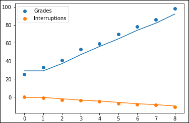
FIGURE 4-2: The KNN approach models the data differently than multiple linear regression.
Implementing KNN Classification
No matter if the problem is to guess a number or a class, the idea behind the learning strategy of the K-Nearest Neighbors (KNN) algorithm is always the same. The algorithm finds the most similar observations to the one you have to predict and from which you derive a good intuition of the possible answer by averaging the neighboring values, or by picking the most frequent answer class among them.
The learning strategy in a KNN is more like memorization. It's just like remembering what the answer should be when the question has certain characteristics (based on circumstances or past examples) rather than really knowing the answer, because you understand the question by means of specific classification rules. In a sense, KNN is often defined as a lazy algorithm because no real learning is done at the training time — just data recording.
Being a lazy algorithm implies that KNN is quite fast at training but very slow at predicting. (Most of the searching activities and calculations on the neighbors is done at that time.) It also implies that the algorithm is quite memory intensive because you have to store your dataset in memory (which means that the number of possible applications is limited when dealing with big data). Ideally, KNN can make the difference when you’re working on classification and you have many labels to deal with (for instance, when a software agent posts a tag on a social network or when proposing a product-selling recommendation). KNN can easily deal with hundreds of labels, whereas other learning algorithms have to specify a different model for each label.
Usually, KNN works out the neighbors of an observation after using a measure of distance such as Euclidean (the most common choice) or Manhattan (works better when you have many redundant features in your data). No absolute rules exist concerning what distance measure is best to use. It really depends on the implementation you have. You also have to test each distance as a distinct hypothesis and verify by cross-validation as to which measure works better with the problem you’re solving.
The example in this section answers the question of whether someone should drive based on conditions. The first condition is pertains to the road: Dry, Damp, or Flooded. The second condition is the environment: Sunny, Cloudy, or Raining. These conditions are the features used to create the input for the model. The third element is the target variable, which simply says No or Yes based on the two conditions. Here is the data used for the example:
road = ['Dry', 'Dry', 'Dry', 'Damp', 'Damp', 'Damp',
'Flooded', 'Flooded', 'Flooded']
weather = ['Sunny', 'Cloudy', 'Raining', 'Sunny',
'Cloudy', 'Raining', 'Sunny', 'Cloudy',
'Raining']
drive = ['Yes', 'Yes', 'Yes', 'Yes', 'Maybe', 'No', 'No',
'No', 'No']
Obviously, the computer would have difficulty using the labels provided, so you need to encode them in some way. For example, you could encode Damp as 0, Dry as 1, and Flooded as 2. Fortunately, Scikit-learn performs this task for you, as shown here:
from sklearn import preprocessing
encoder = preprocessing.LabelEncoder()
roadEnc = encoder.fit_transform(road)
print(roadEnc)
weatherEnc = encoder.fit_transform(weather)
print(weatherEnc)
driveEnc = encoder.fit_transform(drive)
print(driveEnc)
The output shows that the encoder automatically encodes the data in alphabetical order so that even though Sunny comes first in the weather list, it appears as a 2 in the encoding:
[1 1 1 0 0 0 2 2 2]
[2 0 1 2 0 1 2 0 1]
[1 1 1 1 1 0 0 0 0]
Before you go further, you must combine the features into a single list, like this:
features = list(zip(roadEnc, weatherEnc))
print(features)
You end up with a series of tuples that match every road condition with a weather condition, like this:
[(1, 2), (1, 0), (1, 1), (0, 2), (0, 0), (0, 1), (2, 2),
(2, 0), (2, 1)]
At this point, you can fit the model, ask a question, and get a result. The following code shows how the model performs this task for damp and cloudy conditions:
answers = ['Maybe', 'No', 'Yes']
driveModel = KNeighborsClassifier(n_neighbors=3,
metric='manhattan')
driveModel.fit(features, driveEnc)
prediction = driveModel.predict([[0, 0]])
print('Should I drive? {0}'.format(
answers[prediction[0]]))
The output shows that the model is undecided in this particular case:
Should I drive? Maybe